Integer quantum Hall transition in the presence of a long-range-correlated quenched disorder

Abstract

We theoretically study the effect of long-ranged inhomogeneities on the critical properties of the integer quantum Hall transition. For this purpose we employ the real-space renormalization-group (RG) approach to the network model of the transition. We start by testing the accuracy of the RG approach in the absence of inhomogeneities, and infer the correlation length exponent $\nu=2.39$ from a broad conductance distribution. We then incorporate macroscopic inhomogeneities into the RG procedure. Inhomogeneities are modeled by a smooth random potential with a correlator which falls off with distance as a power law, $r^{-\alpha}$. Similar to the classical percolation, we observe an enhancement of $\nu$ with decreasing $\alpha$. Although the attainable system sizes are large, they do not allow one to unambiguously identify a cusp in the $\nu(\alpha)$ dependence at $\alpha_{c}=2/\nu$, as might be expected from the extended Harris criterion. We argue that the fundamental obstacle for the numerical detection of a cusp in the quantum percolation is the implicit randomness in the Aharonov-Bohm phases of the wave functions. This randomness emulates the presence of a short-range disorder alongside the smooth potential.

]

I Introduction

The critical behavior of electron wave functions in the vicinity of the integer quantum Hall (QH) transition is now well understood.[1] That is, the localization length diverges as $\varepsilon^{-\nu}$, where $\varepsilon$ is the deviation from the critical energy. The most accurate value of the exponent $\nu$ extracted from numerical simulations is $\nu=2.35\pm 0.03$.[2] On the experimental side, the study of the critical behavior of the resistance in the transition region at strong magnetic field $B$ has a long history which can be conventionally divided into three periods.

(a)

The first experimental works [3, 4, 5, 6, 7, 8, 9] reported a narrowing of the transition peak with temperature $T$, as $T^{\kappa}$ with $\kappa\sim 0.4$. The spread in the actual value of $\kappa\propto 1/\nu$ measured in different experiments was attributed to the difference in the type of disorder in the samples of Refs. [3, 4] and [5]. Another experimental method to explore the critical behavior was employed in Refs. [6] and [7], where $\kappa$ was deduced from the sample size dependence of the width, $\Delta B$, of the transition region. The value of $\kappa$ obtained by this technique appeared to be consistent with temperature measurements of Ref. [5], in the sense that $\kappa$ was found to be sample dependent. On the other hand, it was argued in Ref. [8] that the lack of universality in Refs. [5, 6, 7] has its origin in the long-ranged character of the disorder in GaAs-based heterostructures studied in these works. This is because for a smooth disorder the energy interval within which the electron transport is dominated by localization effects is relatively narrow.[8] The measurements in Refs. [3] and [4] suggesting the universality of $\kappa$ were carried out on In_xGa_1-xAs/InP heterostructures in which disorder is believed to be short-ranged.[10] Despite the disagreement about universality of the exponent $\kappa$, the fact that the narrowing of the plateau transition occurs as $T^{\kappa}$ was not questioned in Refs. [3, 4, 5, 6, 7, 8, 9].

(b)

The absence of scaling was reported first for the QH-insulator transition [11] and then for the plateau-plateau transition.[12] In the latter paper the conclusion about the absence of scaling was drawn from the analysis of the frequency dependence of $\Delta B$ in GaAs/Al_yGa_1-yAs heterostructures (in contrast to the similar analysis in Ref. [13]). That is, the authors of Refs. [11] and [12] concluded, that the width of the transition region saturates as $T\rightarrow 0$. A possible explanation of this behavior [14, 15] is based on the scenario of tunneling between electron puddles with a size larger than the dephasing length. The microscopic origin of these puddles was attributed to sample inhomogeneities.[16, 17, 18]

(c)

Very recent experimental results [19] on scaling of plateau-insulator as well as plateau-plateau QH transitions carried out on the same In_xGa_1-xAs/InP sample as in Ref. [9] suggested that the narrowing of the transition width with temperature follows a power-law dependence $\Delta B\propto T^{\kappa}$ with $\kappa\approx 0.4$. Even when the authors of Ref. [19] analyzed their data using the procedure of Ref. [11], i.e., by plotting the logarithm of the longitudinal resistance versus $\Delta B$, they obtained straight lines with slopes proportional to $T^{\kappa^{\prime}}$ with $\kappa^{\prime}\approx 0.55$. They attributed the difference between $\kappa$ and $\kappa^{\prime}$ to the marginal dependence of the critical resistance on $T$. It was also speculated in Ref. [19] that this dependence most likely results from macroscopic inhomogeneities in the sample. In the latest papers [20, 21, 22] the frequency dependence of the QH transition width was studied. The results did not support the saturation of the width,[11, 12] but rather confirmed the scaling hypothesis.

Summarizing, it is now conclusively established that insulator-plateau and plateau-plateau transitions exhibit the same critical behavior. It is also recognized that macroscopic inhomogeneities can either mask the scaling or alter the value of $\kappa$.[19]

On the theoretical side, in all previous considerations inhomogeneities were incorporated into the theory through a spatial variation of the local resistivity.[14, 15, 16, 17, 18, 23] In other words, all existing theories are either ”homogeneous quantum coherent” or ”inhomogeneous incoherent”. Meanwhile, there is another scenario which has never been explored. Close to the transition the quantum localization length $\xi$ becomes sufficiently large. Then the long-ranged disorder can affect the character of the divergence of $\xi$. At this point we recall the classical limit,[24, 25] in which the long-ranged disorder does affect the value of the critical exponent in the percolation problem. Obviously, when the disorder is long-ranged but has a finite correlation radius, one should not expect any changes in the critical behavior. The principle finding of Refs. [24] and [25] is that the critical exponent can change when the correlator of the disorder $\langle V({\bf r})V({\bf r^{\prime}})\rangle$ falls off with distance as a power law, i.e., $\propto|{\bf r}-{\bf r^{\prime}}|^{-\alpha}$, (quenched disorder). According to Refs. [24] and [25] the critical exponent of the classical percolation $\nu=4/3$ crosses over to $\nu=2/\alpha$ for $\alpha<3/2$, i.e., when the decay of the correlator is slow enough. In the present paper we study the effects of quenched disorder on quantum percolation. The latter is known to describe the localization-delocalization transition for a two-dimensional (2D) electron in a strong magnetic field. As a model of quantum percolation we employ the Chalker-Coddington (CC) model [26] which is one of the main ”tools” for the quantitative study of the QH transition.[27, 28, 29, 30, 31, 32, 33, 34, 35, 36, 37, 38] The CC model is a strong magnetic field (chiral) limit of a general network model, first introduced by Shapiro [39] and later utilized for the study of localization-delocalization transitions within different universality classes.[40, 41, 42, 43, 44, 45] In addition to describing the QH transition, the CC model applies to a much broader class of critical phenomena since the correspondence between the CC model and thermodynamic, field-theory and Dirac-fermions models [46, 47, 48, 49, 50, 51, 52, 53, 54] was demonstrated.

In order to study the role of the quenched disorder on the localization-delocalization transition we treat the CC model within the real-space renormalization group (RG) approach. First, in Sec. II we check the accuracy of the RG approach, and show that it provides a remarkably accurate description of the QH transition. In Sec. III we extend the RG approach to incorporate the quenched disorder. Concluding remarks are presented in Sec. IV.

II Test of the RG approach to the CC model

A Description of the RG approach

As mentioned in Sec. I, the CC model is a chiral limit of the general network model.[39] However, it was originally derived from a microscopic picture of electron motion in a strong magnetic field and a smooth potential.[26] Within this picture, the links can be identified with semiclassical trajectories of the guiding centers of the cyclotron orbit, while the nodes correspond to the saddle points (SP’s) at which different trajectories come closer than the Larmour radius. For simplicity, the nodes were placed on a square lattice. We will use an equivalent, but slightly different graphical representation of the CC network shown in Fig. 1. In this representation the centers of the trajectories of the guiding centers are placed on a square lattice and play the role of nodes, whereas the SP’s should be identified with links.

We now apply a real-space RG approach [55, 56] to the CC network.[57, 58] The RG approach is based on the assumption that a certain part of the network containing several SP’s, the RG unit, represents the entire network. This unit is then replaced through the RG transformation by a single super-SP with an $S$ matrix determined by the $S$ matrices of the constituting SP’s. The network of super-SP’s is then treated in the same way as the original network. Successive repetition of the RG transformation yields the information about the $S$ matrix of very large samples, since, after each RG step, the effective sample size grows by a certain factor determined by the geometry of the original RG unit. Obviously, a single RG unit is a rather crude approximation of the network. Therefore, prior to applying the RG approach to the study of the quantum Hall transition in the presence of quenched disorder, we first check the accuracy of this approach for the conventional, uncorrelated case, where the comparison with the results of direct numerical simulations is possible.

The RG unit we use is extracted from a CC network on a regular 2D square lattice as shown in Fig. 1. A super-SP consists of five original SP’s by analogy to the RG unit employed for the 2D bond percolation problem.[59, 60, 61] As in any RG scheme, the unit shown in Fig. 1 leaves out a number of bonds of the original lattice. Nevertheless, it is well known that the application of this scheme to the classical case yields very accurate results.[59]

Between the SP’s an electron travels along equipotential lines, and accumulates a certain Aharonov-Bohm phase. Different phases are uncorrelated, which reflects the randomness of the original potential landscape. Each SP can be described by two equations relating the wave-function amplitudes in incoming and outgoing channels. This results in a system of ten linear equations, the solution of which yields the following expression for the transmission coefficient of the super-SP (Ref. [55]):

[

$$t^{\prime}=\left|\frac{t_{1}t_{5}(r_{2}r_{3}r_{4}e^{\imath\Phi_{2}}-1)+t_{2}t_{4}e^{\imath(\Phi_{3}+\Phi_{4})}(r_{1}r_{3}r_{5}e^{-\imath\Phi_{1}}-1)+t_{3}(t_{2}t_{5}e^{\imath\Phi_{3}}+t_{1}t_{4}e^{\imath\Phi_{4}})}{(r_{3}-r_{2}r_{4}e^{\imath\Phi_{2}})(r_{3}-r_{1}r_{5}e^{\imath\Phi_{1}})+(t_{3}-t_{4}t_{5}e^{\imath\Phi_{4}})(t_{3}-t_{1}t_{2}e^{\imath\Phi_{3}})}\right|\quad.$$ (1)

] Here $t_{i}$ and $r_{i}=(1-t_{i}^{2})^{1/2}$ are, respectively, the transmission and reflection coefficients of the constituting SP’s; $\Phi_{j}$ are the phases accumulated along the closed loops (see Fig. 1). Equation (1) is the RG transformation, which allows one to generate (after averaging over $\Phi_{j}$) the distribution $P(t^{\prime})$ of the transmission coefficients of super-SP’s using the distribution $P(t)$ of the transmission coefficients of the original SP’s. Since the transmission coefficients of the original SP’s depend on the electron energy $\varepsilon$, the fact that delocalization occurs at $\varepsilon=0$ implies that a certain distribution, $P_{\text{c}}(t)$ — with $P_{\rm c}(t^{2})$ being symmetric with respect to $t^{2}=\frac{1}{{2}}$ — is the fixed point (FP) of the RG transformation Eq. (1). The distribution $P_{\text{c}}(G)$ of the dimensionless conductance $G$ can be obtained from the relation $G=t^{2}$, so that $P_{\text{c}}(G)\equiv P_{\text{c}}(t)/2t$.

B Critical exponent within the RG approach

Since the dimensionless SP height $z_{i}$ and the transmission coefficient $t_{i}$ at $\varepsilon=0$ are related as $t_{i}=(e^{z_{i}}+1)^{-1/2}$, transformation (1) determines the height of a super-SP through the heights of the five constituting SP’s. Correspondingly, the distribution $P(G)$ determines the distribution $Q(z)$ of the SP heights via $Q(z)=P(G)(dG/dz)=\frac{1}{4}\cosh^{-2}(z/2)P\left[(e^{z}+1)^{-1}\right]$. In fact, $Q(z)$ is not a characteristic of the actual SP’s, but rather, as we will see below, represents a convenient parametrization of the conductance distribution.

The language of the SP heights provides a natural way to extract the critical exponent $\nu$. Suppose that the RG procedure starts with an initial distribution, $Q_{0}(z)=Q_{c}(z-z_{0})$, that is shifted from the critical distribution, $Q_{c}(z)$, by a small $z_{0}\propto\varepsilon$. Since $z_{0}\ll 1$, the first RG step would yield $Q_{c}(z-\tau z_{0})$ with some number $\tau$ independent of $z_{0}$. After $n$ steps the center of the distribution will be shifted by $z_{{\rm max},n}=\tau^{n}z_{0}$, while the sample size will be magnified by $2^{n}$. At the $n$th step corresponding to $z_{{\rm max},n}\sim 1$ a typical SP is no longer transmittable. Then the localization length $\xi$ should be identified with $2^{n}\propto z_{0}^{-\nu}\propto\varepsilon^{-\nu}$, with $\nu=\ln 2/\ln\tau$. When the RG procedure is carried out numerically, one should check that $z_{0}$ is small enough so that $z_{{\rm max},n}\propto z_{0}$ for large enough $n$. Consequently, the working formula for the critical exponent can be presented as

$$\nu=\frac{\ln 2^{n}}{\ln\left(\frac{z_{{\rm max},n}}{z_{0}}\right)}$$ (2)

which should be independent of $n$ for large $n$.

C Numerical results

In order to find the FP conductance distribution $P_{\text{c}}(G)$, we start from a certain initial distribution of transmission coefficients, $P_{0}(t)$ (see below). The distribution is discretized in at least $1000$ bins, such that the bin width is typically $0.001$ for the interval $t\in[0,1]$. From $P_{0}(t)$, we obtain $t_{i}$, $i=1,\ldots,5$, and substitute them into the RG transformation [Eq. (1)]. The phases $\Phi_{j}$, $j=1,\ldots,4$ are chosen randomly from the interval $\Phi_{j}\in[0,2\pi]$. In this way we calculate at least $10^{7}$ super-transmission coefficients $t^{\prime}$. The obtained histogram $P_{1}(t^{\prime})$ is then smoothed using a Savitzky-Golay filter [62] in order to decrease statistical fluctuations. At the next step we repeat the procedure using $P_{1}$ as an initial distribution. We assume that the iteration process has converged when the mean-square deviation $\int{dt[P_{n}(t)-P_{n-1}(t)]^{2}}$ of the distribution $P_{n}$ and its predecessor $P_{n-1}$ deviate by less than $10^{-4}$.

We are now able to study samples with short-ranged disorder. The actual initial distributions, $P_{0}(t)$, were chosen in such a way that corresponding conductance distributions, $P_{0}(G)$, were either uniform or parabolic, or identical to the FP distribution found semianalytically in Ref. [55]. All these distributions are symmetric with respect to $G=0.5$. We find that, regardless of the choice of the initial distribution, after $5$–$10$ steps the RG procedure converges to the same FP distribution which remains unchanged for another $4$–$6$ RG steps. Small deviations from symmetry about $G=0.5$ finally accumulate due to numerical instabilities in the RG procedure, so that typically after $15$–$20$ iterations the distribution becomes unstable and flows towards one of the classical FP’s $P(G)=\delta(G)$ or $P(G)=\delta(G-1)$. We note that the FP distribution can be stabilized by forcing $P_{n}(G)$ to be symmetric with respect to $G=0.5$ in the course of the RG procedure.

Figure 2 illustrates the RG evolution of $P(G)$ and $Q(z)$. In order to reduce statistical fluctuations we average the FP distributions obtained from different $P_{0}(G)$’s. The FP distribution $P_{\text{c}}(G)$ exhibits a flat minimum around $G=0.5$, and sharp peaks close to $G=0$ and $G=1$. It is symmetric with respect to $G\approx 0.5$ with $\langle G\rangle=0.498\pm 0.004$, where the error is the standard error of the mean of the obtained FP distribution. The FP distribution $Q_{c}(z)$ is close to Gaussian.

We now turn to the critical exponent $\nu$. As a result of the general instability of the FP distribution, an initial shift of $Q_{c}(z)$ by a value $z_{0}$ results in the further drift of the maximum position, $z_{{\rm max},n}$, away from $z=0$ after each RG step. As expected, $z_{{\rm max},n}$ depends linearly on $z_{0}$. This dependence is shown in Fig. 3 (inset) for different $n$ from $1$ to $8$. The critical exponent is then calculated from the slope according to Eq. (2). Figure 3 illustrates how the critical exponent converges with $n$ to the value $2.39\pm 0.01$. The error corresponds to a confidence interval of $95\%$ as obtained from the fit to a linear behavior.

Due to the high accuracy of our calculation of $P_{\text{c}}(G)$, we were able to reliably determine many central moments $\langle(G-\langle G\rangle)^{m}\rangle$ of the FP distribution $P_{\text{c}}(G)$. These moments are plotted in Fig. 4.

D Comparison with previous simulations

By dividing the CC network into units, the RG approach completely disregards the interference of the wave-function amplitudes between different units at each RG step. For this reason it is not clear to what extent this approach captures the main features and reproduces the quantitative predictions at the QH transition. Therefore, a comparison of the RG results with the results of direct simulations of the CC model is crucial. These direct simulations are usually carried out by employing either the quasi-1D version [63] or the 2D version [64] of the transfer-matrix method. The results of application of the version of Ref. [63] to the CC model are reported in Refs. [26] and [27]. In Refs. [65, 66, 67] the version of Ref. [64] was utilized. For the critical exponent the values $\nu=2.5\pm 0.5$ (Ref. [26]) and later $\nu=2.4\pm 0.2$ (Ref. [27]) were obtained. Note that our result is in excellent agreement with these values, and is also consistent with the most precise $\nu=2.35\pm 0.03$.[2] This already indicates a remarkable accuracy of the RG approach. In Refs. [65, 66, 67] the critical distribution $P_{\text{c}}(G)$ of the conductance was studied. $P_{\text{c}}(G)$ was found to be broad, which is in accordance with Fig. 2. However, a more detailed comparison is impossible, since the results of the simulations [65, 66, 67] do not obey the electron-hole symmetry condition $P_{\text{c}}(G)=P_{\text{c}}(1-G)$. On the other hand, within the RG approach, the latter condition is satisfied automatically. Nevertheless, we can compare the moments of $P_{\text{c}}(G)$ to those calculated in Refs. [65] and [66]. They are presented in Fig. 4. In Ref. [66] only the standard deviation $\left(\langle G^{2}\rangle-\langle G\rangle^{2}\right)^{1/2}\approx 0.3$ was computed. Our result is $0.316$. In Ref. [65] the moments were fitted by two analytical functions, which are also shown in Fig. 4. They agree with our calculations up to the sixth moment. Here we point out that the moments obtained in Ref. [65] can hardly be distinguished from the moments of a uniform distribution. This reflects the fact that $P_{\text{c}}(G)$ is practically flat except for the peaks close to $G=0$ and $G=1$.

In Refs. [68] and [69] $P_{\text{c}}(G)$ was studied by methods which are not based on the CC model. Both works reported a broad distribution $P_{\text{c}}(G)$. In Ref.  [68] $P_{\text{c}}(G)$ was found to be almost flat. The major difference between Ref. [68] and Fig. 2 is the behavior of $P_{\text{c}}(G)$ near the points $G=0$ and $1$. That is, $P(G)$ drops in Ref. [68] to zero at the ends, while Fig. 2 exhibits maxima. In Ref. [69] the behavior of $P_{\text{c}}(G)$ is qualitatively similar to Fig. 2, with maxima at $G=0$ and $1$. However, the statistics in Ref. [69] are rather poor, which again rules out the possibility of a more detailed comparison with our results.

Finally, we point out that our results agree completely with Refs. [70, 71, 72] where a similar RG treatment of the CC model was carried out. Our numerical data have a higher resolution, and show significantly less statistical noise. This is because we took advantage of faster computation by using the analytical solution of the RG [Eq. (1)].[55] Also, note that, in Refs. [70] and [72] the critical exponent $\nu$ was calculated using a procedure different from that described in Sec. II B. Nevertheless, the values of $\nu$ determined by both methods are close. We emphasize that a systematic improvement of the RG procedure, i.e., by inclusion of more than five SP’s into the basic RG unit as reported in Refs. [70, 71, 72], leads to similar results. The critical distribution of the conductance was also studied experimentally [73, 74] in mesoscopic QH samples. Although an almost uniform conductance distribution consistent with theoretical predictions was found in Ref. [73], further detailed analysis of the mesoscopic pattern [74] has revealed the crucial role of the charging effects, which were neglected in all theoretical studies.

We conclude that the test of the RG approach against other simulations proves that this approach provides a very accurate quantitative description of the QH transition. It can now be used to study the influence of long-ranged correlations.

III Macroscopic inhomogeneities

A General considerations

A natural way to incorporate a quenched disorder into the CC model is to ascribe a certain random shift, $z_{Q}$, to each SP height, and to assume that the shifts at different SP positions, ${\bf r}$ and ${\bf r}^{\prime}$, are correlated as

$$\langle z_{Q}({\bf r})z_{Q}({\bf r}^{\prime})\rangle\propto|{\bf r}-{\bf r}^{\prime}|^{-\alpha},$$ (3)

with $\alpha>0$. After this, the conventional transfer-matrix methods of Refs. [63] and [64] could be employed for numerically precise determination of $\langle G\rangle$, the distribution $P_{\text{c}}(G)$, its moments, and most importantly, the critical exponent, $\nu$. However, the transfer-matrix approach for a 2D sample is usually limited to fairly small sizes (e.g., up to $128$ in Ref. [67]) due to the numerical complexity of the calculation. Therefore, the spatial decay of the power-law correlation by, say, more than an order in magnitude is hard to investigate for small $\alpha$. In principle the quasi-1D transfer-matrix method [26, 63] can easily handle such decays at least in the longitudinal direction, where typically a few million lattice sites are considered iteratively. A major drawback, however, is the numerical generation of power-law correlated randomness since no iterative algorithm is known.[75, 76] This necessitates the complete storage of different samples of correlated SP height landscapes,[77] and the advantage of the iterative transfer-matrix approach is lost. Furthermore, in order to deduce the critical exponent,[27] one needs to perform finite-size scaling [63] with transverse sizes that should also be large enough to capture the main effect of the power-law disorder in the transverse direction. Consequently, even for a single transfer-matrix sample, the memory requirements add up to gigabytes.

On the other hand, the RG approach is perfectly suited to study the role of the quenched disorder. First, after each step of the RG procedure, the effective system size doubles. At the same time, the magnitude of the smooth potential, corresponding to the spatial scale $r$, falls off with $r$ as $r^{-\alpha/2}$. As a result, the modification of the RG procedure due to the presence of the quenched disorder reduces to a rescaling of the disorder magnitude by a constant factor $2^{-\alpha/2}$ at each RG step. Second, the RG approach operates with the conductance distribution, $P_{n}(G)$, which carries information about all the realizations of the quenched disorder within a sample of a size $2^{n}$. This is in contrast to the transfer-matrix approach,[63, 64] within which a small increase of the system size requires the averaging over the quenched disorder realizations to be conducted again.

In order to find out whether or not the critical behavior is affected by the quenched disorder, the following argument was put forward in Ref. [24]. In the absence of the quenched disorder, the correlation length, $\xi_{0}$, for a given energy $z_{Q}$ in the vicinity of the transition is proportional to $z_{Q}^{-\nu}$. Now consider a sample with an area $A=\xi_{0}^{2}$. The variance of the quenched disorder within the sample is given by

$$\begin{array}[]{lll}\Delta_{0}^{2}&=&\frac{1}{A^{2}}\left\langle\int_{A}d^{2}rz_{Q}({\bf r})\int_{A}d^{2}r^{\prime}z_{Q}({\bf r^{\prime}})\right\rangle\\ &=&\frac{1}{A^{2}}\int_{A}d^{2}r\int_{A}d^{2}r^{\prime}\langle z_{Q}({\bf r})z_{Q}({\bf r^{\prime}})\rangle\\ &\propto&\xi_{0}^{-2}\int_{0}^{\xi_{0}}drr^{1-\alpha},\end{array}$$ (4)

where the last relation follows from Eq. (3).

The critical behavior remains unaffected by the quenched disorder if the condition $\Delta_{0}^{2}/z_{Q}^{2}\rightarrow 0$ as $z_{Q}\rightarrow 0$ is met. Using Eq. (4), the ratio $\Delta_{0}^{2}/z_{Q}^{2}$ can be presented as

$$\frac{\Delta_{0}^{2}}{z_{Q}^{2}}\propto\left\{\begin{array}[]{ll}z_{Q}^{2\nu-2},&\alpha>2\quad,\\ z_{Q}^{2\nu-2}\ln(z_{Q}^{-\nu}),&\alpha=2\quad,\\ z_{Q}^{\alpha\nu-2},&\alpha<2\quad.\end{array}\right.$$ (5)

We thus conclude that quenched disorder is irrelevant when

$$\begin{array}[]{ll}\nu>1,&{\text{for }}\alpha\geq 2,\\ \alpha\nu>2,&{\text{for }}\alpha<2\quad.\end{array}$$ (6)

The first condition corresponds to the original Harris criterion [78] for uncorrelated disorder, while the second condition is the extended Harris criterion.[24] It yields the critical value of the exponent $\alpha$, i.e., $\alpha_{c}=2/\nu$.

The above consideration suggests the following algorithm. For the homogeneous case all SP’s constituting the new super-SP are assumed to be identical, which means that the distribution, of heights, $Q_{n}(z)$, for all of them is the same. For the correlated case these SP’s are no longer identical, but rather their heights are randomly shifted by the long-ranged potential. In order to incorporate this potential into the RG scheme, $Q_{n}(z_{i})$ should be replaced by $Q_{n}(z_{i}-\Delta^{(n)}_{i})$ for each SP, $i$, where $\Delta^{(n)}_{i}$ is the random shift. Then the power-law correlation of the quenched disorder enters into the RG procedure through the distribution of $\Delta^{(n)}_{i}$. That is, for each $n$ the distribution is Gaussian with the width $\beta(2^{n})^{-\alpha/2}$. For large enough $n$ the critical behavior should not depend on the magnitude $\beta$, but on the power, $\alpha$, only.

B Numerical results

Here we report the results of the application of the algorithm outlined in the previous section. First, we find that for all values of $\alpha>0$ in correlator (3) the FP distribution is identical to the uncorrelated case within the accuracy of our calculation. In particular, $\langle G\rangle=0.498$ is unchanged. However, the convergence to the FP is numerically less stable than for uncorrelated disorder due to the correlation-induced broadening of $Q_{n}(z)$ during each iteration step. In order to compute the critical exponent $\nu(\alpha)$ we start the RG procedure from $Q_{0}(z-z_{0})$, as in the uncorrelated case, but, in addition, we incorporate the random shifts caused by the quenched disorder in generating the distribution of $z$ at each RG step. The results shown in Fig. 5 illustrate that for increasing long-ranged character of the correlation (decreasing $\alpha$) the convergence to a limiting value of $\nu$ slows down drastically. Even after eight RG steps (i.e., a magnification of the system size by a factor of $256$), the value of $\nu$ with long-ranged correlations still differs appreciably from $\nu=2.39$ obtained for the uncorrelated case. The RG procedure becomes unstable after eight iterations, i.e., $z_{\text{max},9}$ can no longer be obtained reliably from $Q_{9}(z)$. Unfortunately, for small $\alpha$ the convergence is too slow to yield the limiting value of $\nu$ after eight steps only. For this reason, we are, strictly speaking, unable to unambiguously answer the question whether sufficiently long-ranged correlations result in an $\alpha$-dependent critical exponent $\nu(\alpha)$, or the value of $\nu$ eventually approaches the uncorrelated value of $2.39$. Nevertheless, the results in Fig. 5 indicate that the effective critical exponent exhibits a sensitivity to the long-ranged correlations even after a large magnification by $256\times 256$. Therefore, in realistic samples of finite sizes, macroscopic inhomogeneities are able to affect the results of scaling studies. Note further that as shown in the inset of Fig. 5 there is no simple scaling of $\nu$ values when plotted as function of an renormalized system size $2^{\alpha n/2}$. We emphasize that $\nu(\alpha)$ obtained after eight RG steps always exceeds the uncorrelated value. Thus, our results indicate that macroscopic inhomogeneities must lead to smaller values of $\kappa\propto 1/\nu$. Experimentally, the value of $\kappa$ smaller than $0.42$ was reported in a number of early (see, e.g., Ref. [7] and references therein) as well as recent [79] works. This fact was accounted for by different reasons (such as temperature dependence of the phase breaking time, incomplete spin resolution, valley degeneracy in Si-based metal-oxide-semiconductor field-effect transistors, and inhomogeneity of the carrier concentration in GaAs-based structures with a wide spacer). Briefly, the spread of the $\kappa$ values was attributed to the fact that the temperatures were not low enough to assess the truly critical regime. The possibility of having $\kappa<0.4$ due to the correlation-induced dependence of the effective $\nu$ on the phase-breaking length or, ultimately, on the sample size, as in Fig. 5, was never considered.

Figure 6 shows the values of $\nu$ obtained after the eighth RG step as a function of the correlation exponent $\alpha$ for different dimensionless strengths $\beta$ of the quenched disorder. It is seen that in the domain of $\alpha$, where the values of $\nu$ differ noticeably from $\nu=2.39$, their dependence on $\beta$ is strong. According to the extended Harris criterion, $\nu(\alpha)$ is expected to exhibit a cusp at the $\beta$-independent value $\alpha=\alpha_{c}=2/2.39\approx 0.84$. From our results in Fig. 6, two basic observations can be made. For a small enough magnitude of the long-range disorder, we see a smooth enhancement of $\nu(\alpha)$ with decreasing $\alpha$ without a cusp. Although such a behavior is due to the relatively small number of RG steps, the data might be relevant for realistic samples which have a finite size and a finite phase-breaking length governed by temperature. At the largest $\beta=4$, the cusp eventually shows up but the numerics becomes progressively ambiguous, forbidding us from going to even larger $\beta$. The origin for this strong $\beta$ dependence of our results is a profound difference between the classical and quantum percolation problems. This difference is discussed in the Sec. IV.

IV Discussion

A Classical case

In the classical limit, the motion of an a electron in a strong magnetic field and a smooth potential reduces to the drift of the Larmour circle along the equipotential lines. Correspondingly, the description of the delocalization transition reduces to the classical percolation problem. As mentioned above, for classical percolation the quenched disorder is expected to cause a crossover in the exponent $\nu_{c}$, describing the size of a critical equipotential from $\nu_{c}=4/3$ to $\nu_{c}=2/\alpha$ for $\alpha<3/2$. This prediction[25] was made on the basis of Eq. (4). It was later tested by numerical simulations[75] which utilized the Fourier filtering method to generate a long-range-correlated random potential. The exponent $\nu_{c}(\alpha)$ was studied using the same classical real-space RG method [60] that we utilized above. The values of $\nu_{c}$ inferred for $\alpha>1$ were consistently lower than $2/\alpha$. For example, $\nu_{c}=5$ was found for $\alpha=0.4$,[25] whereas $\nu_{c}=3.4\pm 0.3$ was observed.

The classical version of the delocalization transition is instructive, since it allows one to trace how the critical equipotentials grow in size upon approaching the percolation threshold, and how the quenched disorder affects this growth. Roughly speaking, in the absence of long-ranged correlations, the growth of the equipotential size is due to the attachment of smaller equipotentials to the critical ones. As a result, the shape of a critical equipotential is dendritelike. As the threshold is approached, different critical equipotentials become connected through the narrow “arms” of the dendrite. Long-ranged correlations change this scenario drastically. As could be expected intuitively, and as follows from the simulations,[76] critical equipotentials become more compact due to correlations. In fact, for $\alpha<0.25$, the “arms” play no role,[75] i.e., the morphology of a critical equipotential becomes identical to its “backbone”. As a result, the formation of the infinite equipotential at the threshold occurs through a sequence of “broad” merges of compact critical equipotentials. The correlation-induced enhancement of $\nu_{c}$ indicates that due to these merges the size of the critical equipotential in the close vicinity of the threshold grows faster than in the uncorrelated case. Since our simulations also demonstrate the enhancement of the critical exponent due to the correlations, the main result of the present paper can be formulated as follows: quenched disorder affects classical and quantum percolation in a similar fashion.

B Quantum case

Here we note that there is a crucial distinction between the classical case and the quantum regime of the electron motion considered in the present paper. Indeed, within the classical picture, correlated disorder implies that the motion of the guiding centers of the Larmour orbits in two neighboring regions is completely identical. In our study, we have incorporated the correlation of heights of the saddle points into the RG scheme. At the same time we have assumed that the Aharonov-Bohm phases acquired by an electron upon traversing the neighboring loops are completely uncorrelated. This assumption implies that, in addition to the long-ranged potential, a certain short-ranged disorder causing a spread in the perimeters of neighboring loops of the order of the magnetic length is present in the sample. The consequence of this short-range disorder is the sensitivity of our results to the value of $\beta$ which parametrizes the magnitude of the correlated potential. The presence of this short-range disorder affecting exclusively the Aharonov-Bohm phases significantly complicates the observation of a cusp in the $\nu(\alpha)$ dependence at $\alpha\approx 0.84$, as might be expected from the extended Harris criterion.

Let us elaborate on these complications. A general form of the correlator for long-range disorder is

$$\langle V({\bf r})V({\bf r^{\prime}})\rangle=V_{0}^{2}F\left(\frac{|{\bf r}-{\bf r}^{\prime}|}{l}\right)$$ (7)

where $l$ is the microscopic length; $F(0)=1$, $F(x)\propto x^{-\alpha}$ for $x\gg 1$. Now suppose that the correlator contains an additional short-range term $W_{0}^{2}G(|{\bf r}-{\bf r}^{\prime}|/l)$, with $G(0)=1$ and $G(x)$ falling off much more rapidly than $F(x)$ for $x\gg 1$. The extended Harris criterion implies that this term will not change $\nu(\alpha)$ in an infinite sample. It is obvious, however, that in order to “erase the memory” of short-range disorder, many more RG iterations have to be performed or, equivalently, much larger system sizes should be analyzed. Moreover, the larger the ratio $W_{0}/V_{0}$, the more challenging the numerics becomes. At this point, we emphasize that in quantum percolation the short-range term emulated by the randomness in the phases has a huge magnitude. Indeed, if we choose in the first RG step all five SP’s to be identical with power transmission coefficients equal to $0.5$, then due to the phases, the width of the $Q(z)$ distributions after the first step is already $\pm 2.5$.[55] This translates into an enormously wide spread in the transmission coefficients of effective SP’s ranging from $0.075$ to $0.92$. In order to suppress this intrinsic “quantum white noise”, one either has to perform more RG steps or to increase the magnitude of $V_{0}$ (parameter $\beta$ in the notation of Sec. III). Both strategies are limited by numerical instabilities. In particular, a larger $\beta$ leads to more weight in the tails of the $Q(z)$ distribution in which the uncertainty is maximal. In other words, at large $\beta$ the role of rare realizations is drastically emphasized.

In fact, if we had to draw a quantitative conclusion on the basis of the accuracy we have achieved, we would base it on the curve in Fig. 6 corresponding to the maximal value $\beta=4$. Actually, for this $\beta$, the agreement with the extended Harris criterion is fairly good. In particular, for $\alpha=0.5$, we find $\nu\approx 3$, whereas $2/\alpha=4$.

We also want to point out that the limited number (eight) of RG steps permitted by the numerics nevertheless allows us to trace the evolution of the wave functions from microscopic scales (of the order of the magnetic length) to macroscopic scales (of the order of $5\mu{\rm m}$) which are comparable to the sizes of the samples used in the experimental studies of scaling (see e.g., Refs. [6] and [7]) and much larger than the samples[73, 74] used for the studies of mesoscopic fluctuations.

C Concluding remarks

It was argued for a long time that the enhanced value of the critical exponent $\nu$ extracted from the narrowing of the transition region with temperature has its origin in the long-ranged disorder present in GaAs-based samples. To our knowledge, the present work is the first attempt to quantify this argument. We indeed find that the random potential with a power-law correlator leads to the values of $\nu$ exceeding $\nu\approx 2.35$, which is firmly established for short-ranged disorder. Another qualitative conclusion of our study is that the spatial scale at which the exponent $\nu$ assumes its “infinite-sample” value is much larger in the presence of the quenched disorder than in the uncorrelated case. In fact this scale can be of the order of microns. This conclusion can also have serious experimental implications. That is, even if the sample size is much larger than this characteristic scale, this scale can still exceed the phase-breaking length, which would mask the true critical behavior at the QH transition.

Our numerical results demonstrate that when the critical exponent depends weakly on the sample size (large $n$ in Fig. 5), the “saturated” value of $\nu$ depends crucially on the “strength” $\beta$ of the quenched disorder. Thus it is important to relate this strength to the observable quantities. We can roughly estimate $\beta$ assuming that themicroscopic spatial scale (lattice constant) is the magnetic length, $l$, while the microscopic energy scale (the SP height) is the width of the Landau level. We denote by $\gamma$ a typical fluctuation of the filling factor within a region with size $L$. Then the estimate for $\beta$ is $\beta\sim\gamma\left(L/l\right)^{\alpha/2}$. Naturally, for a given $\gamma$, the larger values of $\alpha$ correspond to the “stronger” quenched disorder parameter $\beta$.

Note, finally, that throughout this paper we have considered the localization of a single electron. The role of electron-electron interactions in the scaling of the integer QH effect was recently addressed in Refs. [80] and [81].

FIG. 1.: Network of SP’s (dashed lines) and equipotential lines (circles) on a square lattice. The RG unit used for Eq. (1) combines five SP’s (numbered thick dashed lines) — in analogy with classical 2D bond percolation RG (Refs. [60] and [61]) — into a super-SP. $\Phi_{1},\ldots,\Phi_{4}$ are the phases acquired by an electron drifting along the contours indicated by the arrows.

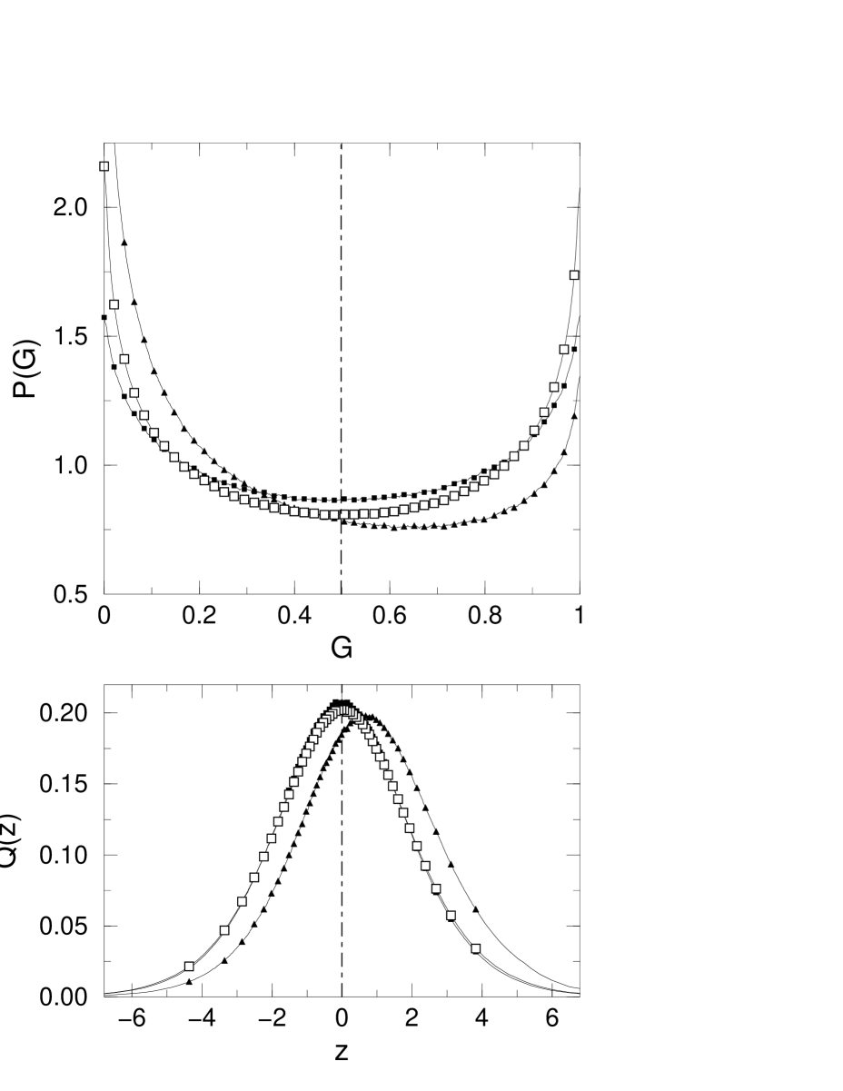
FIG. 2.: Top: $P(G)$ (thin lines) as function of conductance $G$ at a QH plateau-to-plateau transition. Symbols mark every $20$th data point for the initial distribution ($\blacksquare$), the FP ($\Box$) and the distribution for RG step $n=16$ ($\blacktriangle$). The vertical dashed line indicates the average of the FP distribution. Bottom: Corresponding plots for the distribution $Q(z)$ of SP heights.

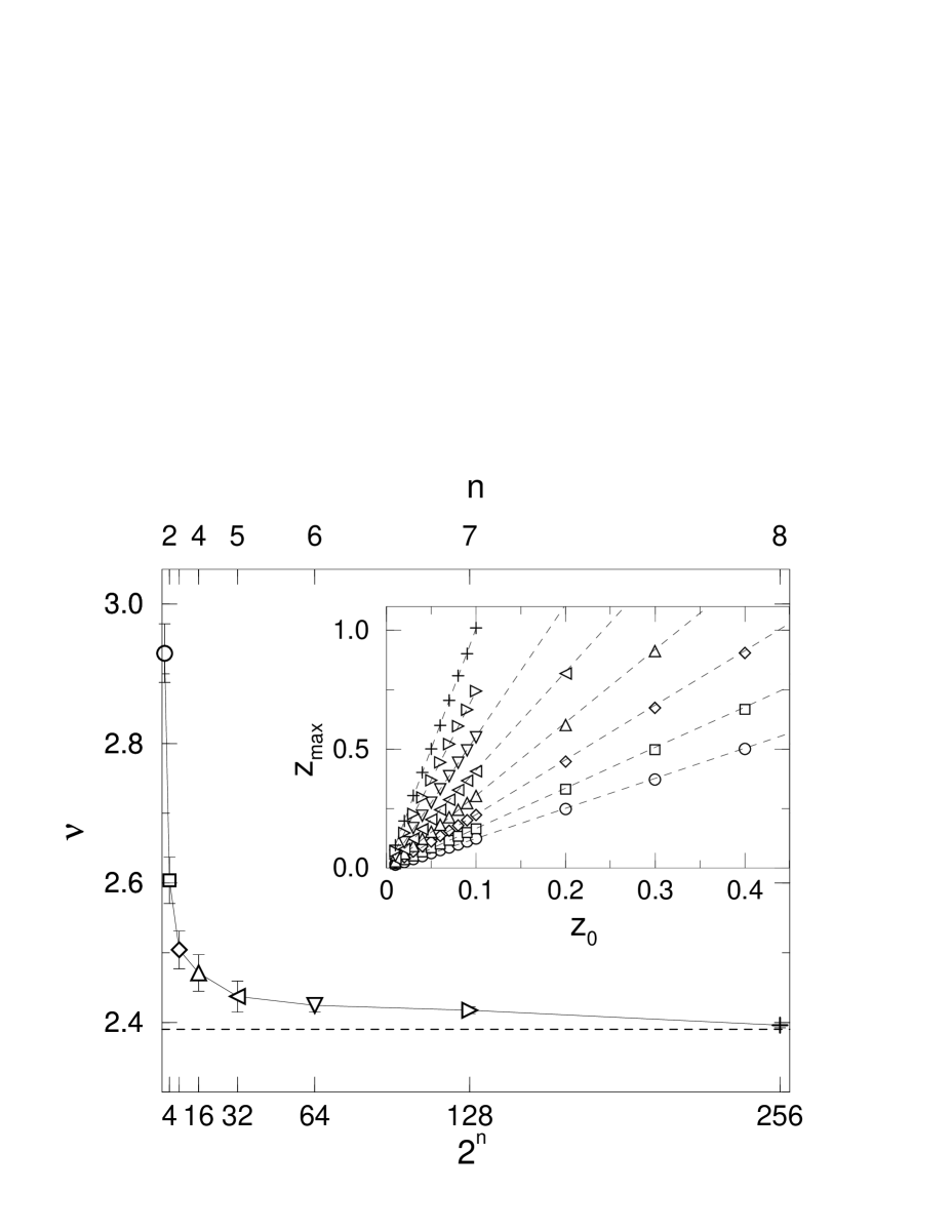
FIG. 3.: Critical exponent $\nu$ obtained by the QH-RG approach as function of effective linear system size $L=2^{n}$ for RG step $n$. The error bars correspond to the error of linear fits to the data. The dashed line shows $\nu=2.39$. Inset: $\nu$ is determined by the dependence of the maximum $z_{{\rm max},n}$ of $Q_{n}(z)$ on a small initial shift $z_{0}$. Dashed lines indicate the linear fits.

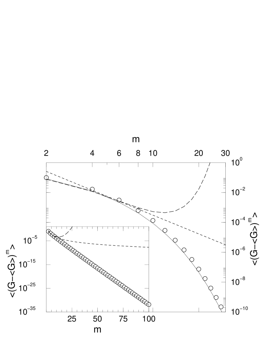
FIG. 4.: Moments $\langle(G-\langle G\rangle)^{m}\rangle$ of the FP distribution $P_{\text{c}}(G)$ ($\circ$). Dashed lines are results from Ref. [65]. The dotted line corresponds to the moments of a constant distribution. Inset: Higher moments of $P_{\text{c}}(G)$ following an exponential behavior. The agreement of data and fit demonstrates the quality of the fit result.

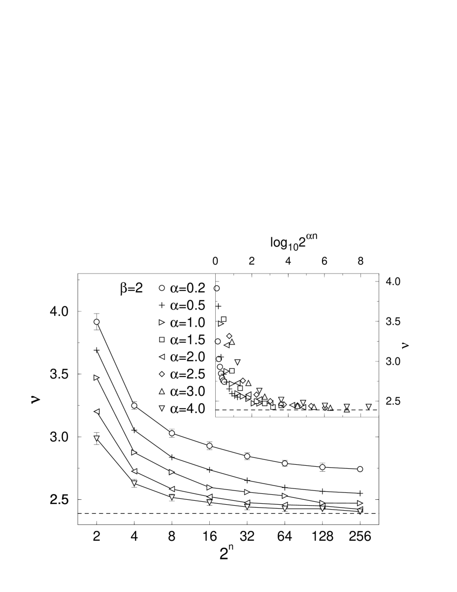
FIG. 5.: Critical exponent $\nu$ obtained by the QH-RG approach as a function of RG scale $2^{n}$ for $\beta=2$ and different correlation exponents $\alpha$. The dashed line indicates $\nu=2.39$, which is the value that we obtain for uncorrelated disorder. For clarity, we show the errors only for $\alpha=0.2$ and $4$. Inset: $\nu$ vs $2^{\alpha n/2}$ does not scale for, e.g., $\beta=2$.

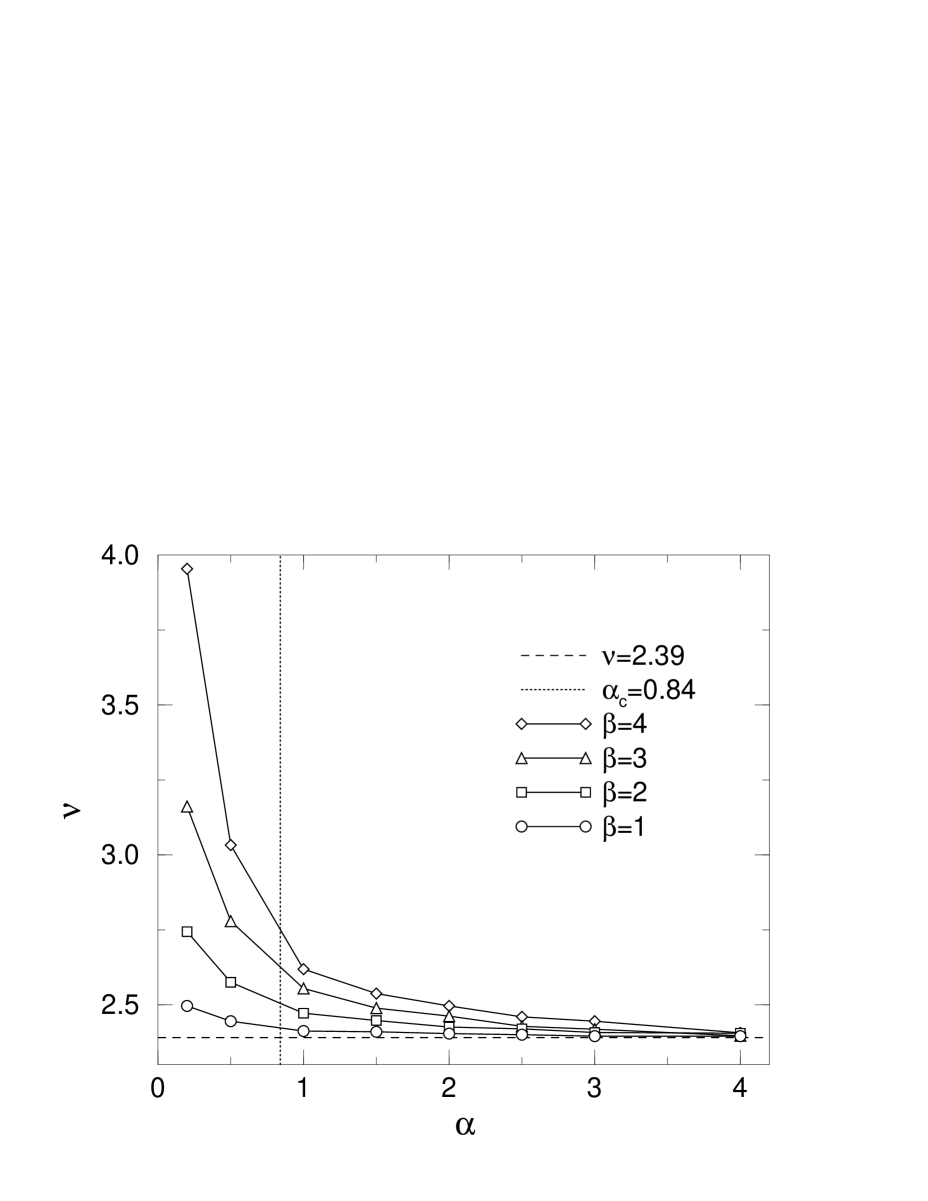
FIG. 6.: Dependence of the critical exponent $\nu$ on correlation exponent $\alpha$ for different $\beta=1,2,3$, and $4$ as obtained after eight QH-RG iterations. The dotted line indicates $\alpha_{c}=0.84$, following from the extended Harris criterion (Ref. [24]) for classical percolation.

- [1] B. Huckestein, Rev. Mod. Phys. 67, 357 (1995).
- [2] B. Huckestein and B. Kramer, Phys. Rev. Lett. 64, 1437 (1990); B. Huckestein, Europhys. Lett. 20, 451 (1992).
- [3] H. P. Wei, D. C. Tsui, and A. M. M. Pruisken, Phys. Rev. B 33, 1488 (1985).
- [4] H. P. Wei, D. C. Tsui, M. A. Paalanen, and A. M. M. Pruisken, Phys. Rev. Lett. 61, 1294 (1988).
- [5] S. Koch, R. J. Haug, K. v. Klitzing, and K. Ploog, Phys. Rev. B 43, 6828 (1991).
- [6] S. Koch, R. J. Haug, K. v. Klitzing, and K. Ploog, Phys. Rev. Lett. 67, 883 (1991).
- [7] S. Koch, R. J. Haug, K. v. Klitzing, and K. Ploog, Phys. Rev. B 46, 1596 (1992).
- [8] H. P. Wei, S. Y. Lin, D. C. Tsui, and A. M. M. Pruisken, Phys. Rev. B 45, 3926 (1992).
- [9] S. W. Hwang, H. P. Wei, L. W. Engel, D. C. Tsui, and A. M. M. Pruisken, Phys. Rev. B 48, 11416 (1993).
- [10] The importance of the character of the disorder (short-ranged vs long-ranged) for the true scaling behavior of the components of the conductivity tensor was recently emphasized by P. T. Coleridge, Phys. Rev. B 60, 4493 (1999); P. T. Coleridge and P. Zawadzki, Solid State Commun. 112, 241 (1999).
- [11] D. Shahar, M. Hilke, C. C. Li, D. C. Tsui, S. L. Sondhi, and M. Razeghi, Solid State Commun. 107, 19 (1998).
- [12] N. Q. Balaban, U. Meirav, and I. Bar-Jospeh, Phys. Rev. Lett. 81, 4967 (1998).
- [13] L. W. Engel, D. Shahar, C. Kurdak, and D. C. Tsui, Phys. Rev. Lett. 71, 2638 (1993).
- [14] E. Shimshoni, A. Auerbach, and A. Kapitulnik, Phys. Rev. Lett. 80, 3352 (1998).
- [15] E. Shimshoni, Phys. Rev. B 60, 10691 (1999).
- [16] S. H. Simon and B. I. Halperin, Phys. Rev. Lett. 73, 3278 (1994).
- [17] I. M. Ruzin, N. R. Cooper, and B. I. Halperin, Phys. Rev. B 53, 1558 (1996).
- [18] N. R. Cooper, B. I. Halperin, C.-K. Hu, and I. M. Ruzin, Phys. Rev. B 55, 4551 (1997).
- [19] R. T. F. van Schaijk, A. de Visser, S. M. Olsthoorn, H. P. Wei, and A. M. M. Pruisken, Phys. Rev. Lett. 84, 1567 (2000).
- [20] F. Kuchar, R. Meisels, K. Dybko, and B. Kramer, Europhys. Lett. 49, 480 (2000).
- [21] F. Hohls, U. Zeitler, R. J. Haug, and K. Pierz, Physica B 298, 88 (2001).
- [22] F. Hohls, U. Zeitler, and R. J. Haug, Phys. Rev. Lett. 86, 5124 (2001).
- [23] We emphasize that sometimes the term ”long-ranged disorder” is also used for a disorder that has a finite correlation radius but which is larger than the magnetic length, see, e.g., F. Evers, A. D. Mirlin, D. G. Polyakov, and P. Wölfle, Phys. Rev. B 60, 8951 (1999). This is different from the present situation.
- [24] A. Weinrib and B. I. Halperin, Phys. Rev. B 27, 413 (1983).
- [25] A. Weinrib, Phys. Rev. B 29, 387 (1984).
- [26] J. T. Chalker and P. D. Coddington, J. Phys. C 21, 2665 (1988).
- [27] D.-H. Lee, Z. Wang, and S. Kivelson, Phys. Rev. Lett. 70, 4130 (1993).
- [28] D. K. K. Lee and J. T. Chalker, Phys. Rev. Lett. 72, 1510 (1994).
- [29] Z. Wang, D.-H. Lee, and X.-G. Wen, Phys. Rev. Lett. 72, 2454 (1994).
- [30] D. K. K. Lee, J. T. Chalker, and D. Y. K. Ko, Phys. Rev. B 50, 5272 (1994).
- [31] V. Kagalovsky, B. Horovitz, and Y. Avishai, Phys. Rev. B 52, R17044 (1995).
- [32] V. Kagalovsky, B. Horovitz, and Y. Avishai, Phys. Rev. B 55, 7761 (1997).
- [33] R. Klesse and M. Metzler, Europhys. Lett. 32, 229 (1995).
- [34] R. Klesse and M. Metzler, Phys. Rev. Lett. 79, 721 (1997).
- [35] I. Ruzin and S. Feng, Phys. Rev. Lett. 74, 154 (1995).
- [36] M. Metzler, J. Phys. Soc. Jpn. 67, 4006 (1998).
- [37] M. Janssen, M. Metzler, and M. R. Zirnbauer, Phys. Rev. B 59, 15836 (1999).
- [38] R. Klesse and M. R. Zirnbauer, Phys. Rev. Lett. 86, 2094 (2001).
- [39] B. Shapiro, Phys. Rev. Lett. 48, 823 (1982).
- [40] P. Freche, M. Janssen, and R. Merkt, in Proceedings of the Ninth International Conference on Recent progress in Many Body Theories, edited by D. Neilson (World Scientific, Singapore, 1998).
- [41] R. Merkt, M. Janssen, and B. Huckestein, Phys. Rev. B 58, 4394 (1998).
- [42] M. Janssen, Phys. Rep. 295, 1 (1998).
- [43] P. Freche, M. Janssen, and R. Merkt, Phys. Rev. Lett. 82, 149 (1999).
- [44] V. Kagalovsky, B. Horovitz, Y. Avishai, and J. T. Chalker, Phys. Rev. Lett. 82, 3516 (1999).
- [45] J. T. Chalker, N. Read, V. Kagalovsky, B. Horovitz, Y. Avishai, and A. W. W. Ludwig, ArXiv: cond-mat/0009463.
- [46] D.-H. Lee, Phys. Rev. B 50, 10788 (1994).
- [47] M. R. Zirnbauer, Ann. Phys. (Leipzig) 3, 513 (1994).
- [48] M. R. Zirnbauer, J. Math. Phys. 38, 2007 (1997).
- [49] I. A. Gruzberg, N. Read, and S. Sachdev, Phys. Rev. B 55, 10593 (1997).
- [50] A. W. W. Ludwig, M. P. A. Fisher, R. Shankar, and G. Grinstein, Phys. Rev. B 50, 7526 (1994).
- [51] Y. B. Kim, Phys. Rev. B 53, 16420 (1996).
- [52] C.-M. Ho and J. T. Chalker, Phys. Rev. B 54, 8708 (1996).
- [53] J. Kondev and J. B. Marston, Nucl. Phys. B 497, 639 (1997).
- [54] J. B. Marston and S. Tsai, Phys. Rev. Lett. 82, 4906 (1999).
- [55] A. G. Galstyan and M. E. Raikh, Phys. Rev. B 56, 1422 (1997).
- [56] D. P. Arovas, M. Janssen, and B. Shapiro, Phys. Rev. B 56, 4751 (1997).
- [57] A very different reformulation of the problem of electron motion in a strong magnetic field in a random potential, which should be suitable for RG analysis, was recently proposed by J. Sinova, V. Meden, and S. M. Girvin, Phys. Rev. B 62, 2008 (2000) and elaborated upon further by J. E. Moore, A. Zee, and J. Sinova, Phys. Rev. Lett. 87, 046801 (2001); S. Boldyrev and V. Gurarie, ArXiv: cond-mat/0009203; V. Gurarie and A. Zee, Int. J. Mod. Phys. B 15, 1225 (2001).
- [58] U. Zülicke and E. Shimshoni, Phys. Rev. B 63, 241301 (2001).
- [59] D. Stauffer and A. Aharony, Introduction to Percolation Theory (Taylor and Francis, London, 1992).
- [60] P. J. Reynolds, W. Klein, and H. E. Stanley, J. Phys. C 10, L167 (1977).
- [61] J. Bernasconi, Phys. Rev. B 18, 2185 (1978).
- [62] W. H. Press, B. P. Flannery, S. A. Teukolsky, and W. T. Vetterling, Numerical Recipes in FORTRAN, 2nd ed. (Cambridge University Press, Cambridge, 1992).
- [63] A. MacKinnon and B. Kramer, Phys. Rev. Lett. 47, 1546 (1981).
- [64] D. S. Fisher and P. A. Lee, Phys. Rev. B 23, 6851 (1981).
- [65] Z. Wang, B. Jovanovic, and D.-H. Lee, Phys. Rev. Lett. 77, 4426 (1996).
- [66] S. Cho and M. P. A. Fisher, Phys. Rev. B 55, 1637 (1997).
- [67] B. Jovanovic and Z. Wang, Phys. Rev. Lett. 81, 2767 (1998).
- [68] X. Wang, Q. Li, and C. M. Soukoulis, Phys. Rev. B 58, 3576 (1998).
- [69] Y. Avishai, Y. Band, and D. Brown, Phys. Rev. B 60, 8992 (1999).
- [70] A. Weymer and M. Janssen, Ann. Phys. (Leipzig) 7, 159 (1998).
- [71] M. Janssen, R. Merkt, and A. Weymer, Ann. Phys. (Leipzig) 7, 353 (1998).
- [72] M. Janssen, R. Merkt, J. Meyer, and A. Weymer, Physica B 256–258, 65 (1998).
- [73] D. H. Cobden and E. Kogan, Phys. Rev. B 54, R17316 (1996).
- [74] D. H. Cobden, C. H. W. Barnes, and C. J. B. Ford, Phys. Rev. Lett. 82, 4695 (1999).
- [75] S. Prakash, S. Havlin, S. Schwartz, and H. E. Stanley, Phys. Rev. A 46, R1724 (1992).
- [76] H. Makse, S. Havlin, M. Schwartz, and H. E. Stanley, Phys. Rev. E 53, 5445 (1996).
- [77] S. Russ, J. W. Kantelhardt, A. Bunde, S. Havlin, and I. Webman, Physica A 266, 492 (1999).
- [78] A. B. Harris, J. Phys. C 7, 1671 (1974).
- [79] G. Landwehr, (private communication); X. C. Zhang, A. Pfeuffer-Jeschke, K. Ortner, V. Hock, H. Buhmann, C. R. Becker, and G. Landwehr, Phys. Rev. B 63, 245305 (2001).
- [80] B. Huckestein and M. Backhaus, Phys. Rev. Lett. 82, 5100 (1999).
- [81] Z. Wang, M. P. A. Fisher, M. Girvin, and J. T. Chalker, Phys. Rev. B 61, 8326 (2000).