Extreme Value Statistics of Hierarchically Correlated Variables: Deviation from Gumbel Statistics and Anomalous Persistence

Abstract

We study analytically the distribution of the minimum of a set of hierarchically correlated random variables $E_{1}$, $E_{2}$, $\dots$, $E_{N}$ where $E_{i}$ represents the energy of the $i$-th path of a directed polymer on a Cayley tree. If the variables were uncorrelated, the minimum energy would have an asymptotic Gumbel distribution. We show that due to the hierarchical correlations, the forward tail of the distribution of the minimum energy becomes highly non universal, depends explicitly on the distribution of the bond energies $\epsilon$ and is generically different from the super-exponential forward tail of the Gumbel distribution. The consequence of these results to the persistence of hierarchically correlated random variables is discussed and the persistence is also shown to be generically anomalous.

PACS numbers: 02.50.-r, 05.40.-a 23 March 2001

The extreme value statistics of random variables is important in various branches of physics, statistics, and mathematics[1, 2, 3]. For example, in the context of disordered systems, the thermodynamics at low temperatures is governed by the statistics of the low energy states. The statistics of extremal quantities also play important roles in binary search problems in computer science[4]. The extreme-value statistics is well understood when the random variables are independent and identically distributed. In this case, depending on the distribution of the random variable, three different universality classes of extreme value statistics are known[3]. Recently there has been an attempt to identify these different universality classes with the different schemes of replica symmetry breaking[5]. A natural question is: what are the universality classes when the random variables are correlated? This question has recently been addressed[6, 5] and it has been conjectured that this class of problems corresponds to the full replica symmetry breaking[5]. To answer this important question, it would thus be useful to derive exact results for the extreme value statistics of correlated variables, whenever possible.

More precisely, let us consider a set of $N$ random variables $E_{1}$, $E_{2}$, $\ldots$, $E_{N}$ drawn from a joint probability distribution $p(E_{1},E_{2},\ldots,E_{N})$. Then the minimum value, $E_{\rm min}={\rm min}\{E_{1},E_{2},\ldots,E_{N}\}$ is also a random variable and one would like to know its probability distribution. Let, $P_{N}(x)=Prob[E_{\rm min}\geq x]$ be the cumulative distribution of the minimum. Then clearly,

$$P_{N}(x)=\int_{x}^{\infty}\dots\int_{x}^{\infty}p(E_{1},E_{2},\dots,E_{N})\prod_{i=1}^{N}dE_{i},$$ (1)

since if the minimum is bigger than $x$, then each of the variables must also be bigger than $x$. When the variables are uncorrelated and each is drawn from the same distribution $p(E)$, the joint distribution factorizes, $p(E_{1},E_{2},\ldots,E_{N})=p(E_{i})\dots p(E_{N})$ and from Eq. (1) one simply gets, $P_{N}(x)=[\int_{x}^{\infty}p(E)dE]^{N}$. If the distribution $p(E)$ is unbounded and decays faster than a power law for large $|E|$, then one can show that for large $N$, $P_{N}(x)$ approaches a scaling form[3], $P_{N}(x)=F[(x+a_{N})/b_{N}]$. Here $a_{N}$ and $b_{N}$ are functions of $N$ and depend explicitly on the distribution $p(E)$, but the scaling function $F(y)$ is independent of $p(E)$ and $N$ and has the universal super-exponential form, $F(y)=\exp[-\exp(y)]$. As a consequence, the distribution of the minimum $P_{\rm min}(y)=-dF/dy=\exp[y-\exp(y)]$ has the universal Gumbel form. There are two other known universality classes when the distribution $p(E)$ is either bounded or has algebraic tails for large $|E|$, but we will not be concerned with these cases in this paper.

The question we focus on here is whether the Gumbel law continues to hold if the random variables are unbounded but correlated. This question has recently been addressed by Carpentier and Le Doussal[6] who developed a renormalization group (RG) approach for logarithmically correlated variables. With logarithmic correlations they found that the cumulative distribution function $F(y)$ behaves (up to some rescaling factors) as, $F(y)=1-y\exp(y)$ in the backward tail region $y\to-\infty$. A pure Gumbel law would have predicted, $F(y)=1-\exp(y)$ as $y\to-\infty$. Thus the Gumbel law is indeed violated in this backward tail region. However, their RG approach can not predict whether the super-exponential forward tail of the Gumbel distribution still holds or not. The question we are interested in is whether strong correlations can also modify the super-exponential forward tail of the Gumbel distribution. If so, this has interesting consequence for the persistence of random variables as we discuss below.

The persistence of random variables, a subject that has generated a lot of recent interest [7], is related to the distribution of the minimum in a simple way. For random variables each with zero mean, the persistence is simply the probability that all of them are positive and is given by $P_{N}(0)$ in Eq. (1). For independent variables, it follows trivially from Eq. (1) that $P_{N}(0)$ decays exponentially with $N$, $P_{N}(0)=\exp(-\theta N)$ where $\theta=-\log[\int_{0}^{\infty}p(E)dE]$. For correlated variables, this problem has been studied for many decades by applied mathematicians who call it the ‘one sided barrier’ problem[8, 9]. It is well known that $P_{N}(0)$ is hard to compute analytically even for Gaussian correlated variables, i.e., when the joint distribution $p(E_{1},E_{2},\ldots,E_{N})$ is a multivariate Gaussian distribution[8, 9, 10]. If the Gaussian variables are arranged on a line and if the correlation between two variables $E_{i}$ and $E_{j}$ decays faster than $1/|i-j|$, then $P_{N}(0)$ is known to decay as $P_{N}(0)\sim\exp(-\theta N)$ for large $N$[9], where the persistence exponent $\theta$ is nontrivial and is known exactly only in very few special cases[8]. It would thus be interesting to know if strong correlations can modify this exponential decay of the persistence for large $N$.

In this paper, we show that the two issues, (a) the possibility of a non-Gumbel forward tail of the distribution of the minimum and (b) the possibility of non-exponential decay of persistence, are related to each other for random variables that are hierarchically correlated. The hierarchical nature of the correlation allows us to derive exact asymptotic results for both the quantities. Our main results are twofold: (i) For the distribution of minimum value, we show that the super-exponential forward tail of the Gumbel law is violated under generic conditions and (ii) as a consequence, the persistence is anomalous, i.e., $P_{N}(0)$ does not decay exponentially under the same generic conditions.

We consider, as a model, the well studied problem of a directed polymer on a tree. This problem was first studied by Derrida and Spohn[11], who were mostly interested in the finite temperature phase transition in this model. Here we focus explicitly on the zero temperature properties. We consider a tree rooted at $O$ (see Fig. 1) and a random energy $\epsilon_{i}$ is associated with every bond of the tree. The variables $\epsilon_{i}$’s are independent and each drawn from the same distribution $\rho(\epsilon)$. A directed polymer of size $n$ goes down from the root $O$ to any of the $2^{n}$ nodes at the level $n$. Thus, there are $N=2^{n}$ possible paths for the polymer of size $n$ and the energy of any of these paths is given by,

$$E_{\rm path}=\sum_{i\in{\rm path}}{\epsilon}_{i}.$$ (2)

The set of $N=2^{n}$ variables $E_{1}$, $E_{2}$, $\ldots$, $E_{N}$ are clearly correlated in a hierarchical (i.e. ultrametric) way and the two point correlation between the energies of any two paths is proportional to the number of bonds they share. We would then like to know the distribution of the minimum energy.

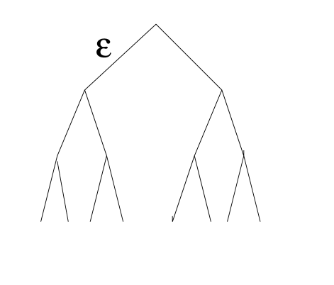
FIG. 1.: Each bond of a Cayley tree has an energy $\epsilon_{i}$.

Clearly, $P_{N}(x)=Prob[E_{\rm min}\geq x]$ is also the probability that all the $N$ paths up to the $n$-th level have energies $\geq x$. Since $N=2^{n}$, let us write, for convenience, $R_{n}(x)=P_{N}(x)$. It is easy to see that $R_{n}(x)$ satisfies the recursion relation,

$$R_{n+1}(x)={\left[\int_{-\infty}^{\infty}d\epsilon\rho(\epsilon)R_{n}(x-\epsilon)\right]}^{2},$$ (3)

with the initial condition, $R_{0}(x)=\theta(-x)$ where $\theta(x)$ is the usual Heaviside step function. This relation is derived by considering various possibilities for the energies of the two bonds emerging from the root $O$ and taking into account that the two subsequent daughter trees are statistically independent. The Eq. (3) was studied in detail in Ref. [12] for several distributions $\rho(\epsilon)$’s with non negative support. In particular, for the bivariate distribution, $\rho(\epsilon)=p\delta(\epsilon-1)+(1-p)\delta(\epsilon)$, the solution of Eq. (3) was shown to undergo a depinning phase transition at $p_{c}=1/2$[12]. Since in this paper we are mostly interested in the persistence of the $E_{i}$ variables, we restrict ourselves subsequently only to symmetric distributions $\rho(\epsilon)$ with zero mean. Defining $R_{n}(x)=Q_{n}^{2}(x)$, Eq. (3) can be recast into,

$$Q_{n+1}(x)=\int_{-\infty}^{\infty}d\epsilon\rho(\epsilon)Q_{n}^{2}(x-\epsilon),$$ (4)

with the initial condition, $Q_{0}(x)=\theta(-x)$ and the boundary conditions, $Q_{n}(x)\to 0$ as $x\to\infty$ and $Q_{n}(x)\to 1$ as $x\to-\infty$.

The Eq. (4) is known[12] to admit a traveling front solution, $Q_{n}(x)=q(x+vn)$ where the front propagates in the negative $x$ direction with a constant velocity $v$ as $n$ increases (see Fig. 2). Substituting $Q_{n}(x)=q(x+vn)$ in Eq. (4), we get

$$q(y)=\int_{-\infty}^{\infty}d\epsilon\rho(\epsilon)q^{2}(y-v-\epsilon),$$ (5)

with the boundary conditions, $q(y)\to 1$ as $y\to-\infty$ and $q(y)\to 0$ as $y\to\infty$, with the front located around $y=0$. The velocity $v$ can then be determined exactly by analyzing the backward tail region, $y\to-\infty$ of the function $q(y)$. In this regime, substituting $q(y)=1-g(y)$ in Eq. (5) and neglecting the terms of $O(g^{2})$, we find that the resulting linear equation admits an exponential solution, $g(y)=\alpha\exp(\lambda y)$ with $\alpha>0$ provided $v$ is related to $\lambda$ via the dispersion relation,

$$v={1\over{\lambda}}\log\left[2\int_{-\infty}^{\infty}d\epsilon\rho(\epsilon)e^{-\lambda\epsilon}\right].$$ (6)

For generic distributions $\rho(\epsilon)$, the function $v_{\lambda}$ has a unique minimum at $\lambda=\lambda^{*}$ and by the general velocity selection principle[13], this minimum velocity, $v_{\lambda^{*}}$ is selected by the front[11, 12].

Thus the cumulative distribution of the minimum energy approaches a scaling form for large $N$, $P_{N}(x)=R_{n}(x)=Q_{n}^{2}(x)\to q^{2}[x+{{v_{\lambda^{*}}}\over{\log 2}}\log N]$, where the function $q(y)$ is given by the solution of Eq. (5) and $v_{\lambda^{*}}$ is determined by minimizing Eq. (6). The question we are interested in is: what is the asymptotic form of $q(y)$ for large $y$? We show below that that for any bounded distribution $\rho(\epsilon)$, the function $q(y)$ for large $y$ indeed has the Gumbel shape, $q(y)\to\exp[-c_{1}\exp(c_{2}y)]$ where $c_{1}$ and $c_{2}$ are positive constants. On the other hand, for unbounded distributions $\rho(\epsilon)$, the Gumbel law breaks down and asymptotic forward tail of $q(y)$ is nonuniversal and is determined explicitly by the distribution $\rho(\epsilon)$. For example, for the exponential distribution, $\rho(\epsilon)=\exp[-|\epsilon|]/2$, we find exactly $q(y)\to\exp(-y)$ for large $y$. For a generic unbounded distribution, one can prove a lower bound, $q(y)>f(y)$ for large $y$, where $f(y)=\int_{y}^{\infty}\rho(\epsilon)d\epsilon$.

FIG. 2.: The traveling front for the function $Q_{n}(x)$ for $n=10$ (the solid line), $20$ (the dashed line) and $30$ (the dotted line) for exponential distribution $\rho(\epsilon)=\exp[-|\epsilon|]/2$. In the inset, we plot the logarithm of the collapsed scaling function $q(x+vn)$ (for different $n$). The scaling function $q(y)$ evidently has an exponential tail for large $y$.

We first focus on the unbounded distributions $\rho(\epsilon)$. Let us first consider the exponential distribution, $\rho(\epsilon)=\exp(-|\epsilon|)/2$. In this case, by first making a change of variable $\epsilon\to y-v-\epsilon$ inside the integrand on the right hand of side of Eq. (5) and then differentiating twice the resulting equation, we get

$${{d^{2}q}\over{dy^{2}}}=q(y)-q^{2}(y-v).$$ (7)

For large $y$, clearly the nonlinear term is negligible since $q(y)$ is small. Using the boundary condition $q(y)\to 0$ as $y\to\infty$ we then get, $q(y)\to A\exp(-y)$ for large $y$ where $A$ is a constant. Thus we get an exponential forward tail instead of the standard super-exponential forward tail of the Gumbel distribution. Note that the velocity $v$ is determined, as before, from the $y\to-\infty$ tail where $q(y)=1-\alpha e^{\lambda y}$ and Eq. (7) gives, $v_{\lambda}=\log[2/(1-\lambda^{2})]/\lambda$ with $0<\lambda<1$, in accordance with the general formula in Eq. (6). The function $v_{\lambda}$ has a unique minimum at $\lambda^{*}=0.603582\dots$ and the chosen front velocity is then, $v_{\lambda^{*}}=1.89899\dots$. In Fig. (2), we show that $Q_{n}(x)$ indeed approaches the scaling form, $Q_{n}(x)\to q(x+v_{\lambda^{*}}n)$ and the tail of the scaling function is given by, $q(y)\sim\exp(-y)$ (see the inset of Fig. (2)) as predicted analytically.

For a generic unbounded distribution it is difficult to derive exact results. However, one can easily derive a lower bound for $q(y)$. From Eq. (5), it is clear that $q(y)\geq\int_{y-v}^{\infty}d\epsilon\rho(\epsilon)q^{2}(y-v-\epsilon)$. This follows since the integrand on the right hand hand side of Eq. (5) is always positive. Since the function $q(y)$ saturates to $1$ very quickly for negative $y$, we can replace $q^{2}(y-v-\epsilon)$ by $1$ on the right hand side of the above lower bound. This gives, for large $y$, $q(y)\geq f(y)$ where $f(y)=\int_{y}^{\infty}\rho(\epsilon)d\epsilon$. For example, for the Gaussian distribution, $\rho(\epsilon)=e^{-\epsilon^{2}/2}/{\sqrt{2\pi}}$, this result indicates that $q(y)$ should decay at most as fast as $f(y)={\rm erfc}(y/{\sqrt{2}})$. Thus, for generic unbounded distributions, the forward tail of the function $q(y)$ for large $y$ is highly nonuniversal and is generally different from the super-exponential forward tail as in the Gumbel distribution.

Next we consider the bounded distributions $\rho(\epsilon)$. The lower bound discussed in the previous paragraph continues to hold for bounded distributions as well, though for large $y$ it trivially becomes zero for distributions with an upper cutoff. To obtain more precisely the behavior of $q(y)$ as $y\to\infty$, we first consider a specific example, $\rho(\epsilon)=a\delta(\epsilon+1)+a\delta(\epsilon-1)+(1-2a)\delta(\epsilon)$ with $0<a<1/2$. The Eq. (5) then becomes,

$$q(y) = a\,q^{2}(y-v-1)+a\,q^{2}(y-v+1)$$ (8)

$$+ (1-2a)q^{2}(y-v),$$ (9)

where the velocity $v=v_{\lambda^{*}}$ is obtained by minimizing Eq. (6) with respect to $\lambda$. In this particular case, we get from Eq. (6),

$$v_{\lambda}={1\over{\lambda}}\log\left[4a\cosh(\lambda)+2(1-2a)\right],$$ (10)

which has a unique minimum at $\lambda=\lambda^{*}(a)$ for all $0<a<1/2$. We then need to analyze the large $y$ behavior of $q(y)$ in Eq. (9) with $v=v_{\lambda^{*}}$. Note that as one increases $y$ from $-\infty$, $q(y)$ remains approximately $1$ up to the back edge of the front at $y=0$ and then starts decreasing to $0$ as $y$ increases beyond $0$. The idea would be to determine $q(y)$ for a fixed large $y$ by iterating Eq. (9) backwards in $y$ till we reach the back edge of the front at $y=0$ where $q(y)\approx 1$. Anticipating a super-exponential decay of $q(y)$ for large $y$, one can neglect the second and the third term on the right hand side of Eq. (9) and iterate the equation retaining only the first term. Iterating $m$ times backward we get,

$$q(y)\approx a^{2^{m}-1}{\left[q\left(y-m(v+1)\right)\right]}^{2^{m}}.$$ (11)

How many iterations do we need to reach $0$ starting from a fixed large $y$? Clearly the required value of $m$ is given by, $m=y/(v+1)$ so that the argument of the function on the right hand side of Eq. (11) becomes $0$. Using $q(0)\approx 1$, we get from Eq. (11) the large $y$ behavior,

$$q(y)\approx a^{2^{y/(v+1)}},$$ (12)

confirming the super-exponential forward tail of $q(y)$ and also justifying, a posteriori, the neglect of the second and the third term in the iteration of Eq. (9). We have verified the analytical prediction in Eq. (12) by direct numerical integration of Eq. (4) with $\rho(\epsilon)=a\delta(\epsilon+1)+a\delta(\epsilon-1)+(1-2a)\delta(\epsilon)$ for $a=1/4$ (see Fig. (3)).

FIG. 3.: The traveling front for the function $Q_{n}(x)$ for $n=100$ (the solid line), $150$ (the dashed line) and $200$ (the dotted line) for the distribution $\rho(\epsilon)=a\delta(\epsilon+1)+a\delta(\epsilon-1)+(1-2a)\delta(\epsilon)$ with $a=1/4$. In the inset, we plot $\log(-\log(q(y)))$ against $y$ which clearly shows the super-exponential decay of the scaling function $q(y)$ for large $y$.

The argument leading to the result in Eq. (12) above uses only the fact that distribution $\rho(\epsilon)$ has an upper cutoff at $\epsilon=1$. Thus we expect that $q(y)$ will always have a super-exponential forward tail as long as the distribution $\rho(\epsilon)$ is bounded with an upper cutoff $\Lambda$. Let us consider another example of a bounded distribution, namely the uniform distribution, $\rho(\epsilon)=[\theta(\epsilon+1)-\theta(\epsilon-1)]/2$. In this case, we get from Eq. (5),

$$q(y)={1\over{2}}\int_{y-v-1}^{y-v+1}dzq^{2}(z).$$ (13)

Differentiating the Eq. (13) with respect to $y$ yields,

$${{dq}\over{dy}}={1\over{2}}q^{2}(y-v+1)-{1\over{2}}q^{2}(y-v-1).$$ (14)

Again we anticipate that $q(y)$ will have a super-exponential tail for large $y$. If so, one can make the approximation, $\log(-dq/dy)\approx\log(q(y))$. Using this in Eq. (14) we iterate the equation backwards as before after dropping the first term on the right hand side of Eq. (14). Using the same line of arguments used in the previous paragraph, we finally get a super-exponential tail for large $y$ as before,

$$q(y)\approx 2^{-2^{y/(v+1)}}.$$ (15)

Note that the velocity $v$ in Eq. (15) has to be determined by minimizing Eq. (6) with a uniform distribution. Thus, in general, for any bounded distribution, we expect that for large $y$

$$q(y)\approx\exp\left[-c\,2^{y/(v+1)}\right],$$ (16)

where the constants $c$ and $v$ depend explicitly on the distribution $\rho(\epsilon)$.

Having established the forward tail behavior of $R_{n}(x)=q^{2}(x+vn)$, we now turn to the persistence. The persistence is simply given by $P_{N}(0)=R_{n}(0)=Q_{n}^{2}(0)=q^{2}(vn)$, where $N=2^{n}$. Thus for large $N$ or equivalently for large $n$, the asymptotic behavior of persistence $P_{N}(0)=q^{2}(vn)$ is governed by the forward tail of the function $q(y)$ for large $y$. Let us first consider the bounded distributions. In this case, using the result from Eq. (16) for $q(y)$, we get the following exact result for persistence for large $N=2^{n}$,

$$P_{N}(0)=Q_{n}^{2}(0)=q^{2}(vn)\approx\exp\left[-2cN^{\alpha}\right],$$ (17)

where $\alpha=v/(v+1)$ and $v$ is determined by minimizing Eq. (6). Thus the persistence has an anomalous stretched exponential decay for large $N$ instead of the standard exponential decay. We have verified this analytical prediction by numerically integrating Eq. (4) for different bounded distributions. In Fig. (4), we show the result for the distribution $\rho(\epsilon)=a\delta(\epsilon+1)+a\delta(\epsilon-1)+(1-2a)\delta(\epsilon)$. In this case, $\alpha=v/(v+1)$ where $v$ is the minimum value of the dispersion relation in Eq. (10) and is clearly a continuous function of the parameter $a$. In the inset of Fig. (4), we compare the analytical prediction for the exponent $\alpha(a)=v/(1+v)$ with that obtained from the numerical integration for various values of $a$. The agreement is evidently very good.

FIG. 4.: The function $\log(-\log(Q_{n}(0)))$, obtained from the numerical integration of Eq. (4), is plotted against $n$ for the distribution $\rho(\epsilon)=a\delta(\epsilon+1)+a\delta(\epsilon-1)+(1-2a)\delta(\epsilon)$ with $a=1/4$. The linear increase with $n$ confirms the stretched exponential decay of $P_{N}(0)=Q_{n}^{2}(0)$ for large $N=2^{n}$. In the inset is shown the value of $\alpha(a)$ calculated analytically (solid line) with that measured numerically by direct integration of Eq. (4) (circles).

We next consider the unbounded distributions such as $\rho(\epsilon)=\exp[-|\epsilon|]/2$. For this exponential distribution, using the asymptotic behavior $q(y)=A\exp(-y)$, we find that for large $N$,

$$P_{N}(0)=Q_{n}^{2}(0)=q^{2}(vn)\sim\exp[-2vn]\sim N^{-\beta},$$ (18)

where $\beta=2v/\log 2$ with $v$, as usual, determined via minimizing Eq. (6). Thus in this case, persistence again decays anomalously but now as a power law with a nonuniversal exponent $\beta$. Again we verified this analytical prediction numerically by directly integrating Eq. (4) with the exponential distribution (see Fig. (5)). For generic unbounded distributions, using the lower bound $q(y)\geq f(y)$ for large $y$ where $f(y)=\int_{y}^{\infty}\rho(\epsilon)d\epsilon$, we get $P_{N}(0)=q^{2}(nv)\geq f^{2}[{v\log N}/\log 2]$, again highly anomalous.

FIG. 5.: The function $\log(Q_{n}(0)))$, obtained from the numerical integration of Eq. (4), is plotted against $n$ for the distribution $\rho(\epsilon)=\exp(-|\epsilon|)/2$. The linear decrease with $n$ confirms the power law decay of $P_{N}(0)=Q_{n}^{2}(0)$ for large $N=2^{n}$ with the exponent $\beta=2v/\log 2$ where $v\approx 1.89$.

In summary, we have investigated in detail the distribution of the minimum energy of a directed polymer on a Cayley tree. We have shown that the hierarchical correlations between the energies of different paths have a considerable effect on the distribution of minimum energy depending on the distribution of bond energies $\rho(\epsilon)$. In the case of bounded distributions $\rho(\epsilon)$ of the bond energies, we have shown that the forward tail has a super-exponential tail as in the Gumbel distribution. However, for unbounded distributions $\rho(\epsilon)$ the forward tail is highly non universal and depends explicitly on the distribution $\rho(\epsilon)$. This rich behavior of the forward tail of the minimum energy distribution is shown to lead to a variety of anomalous behavior for the persistence probability $P_{N}(0)$, ranging from a stretched exponential decay for bounded distributions $\rho(\epsilon)$ to power law decay when $\rho(\epsilon)$ is exponential.

REFERENCES

- [1] E.J. Gumbel, Statistics of Extremes (Columbia University Press, New York, 1958).
- [2] J. Galambos, The Asymptotic Theory of Extreme Order Statistics (R.E. Krieger Publishing Co., Malabar, 1987).
- [3] S.M. Berman, Sojourn Times and the Extremum of Stationary Sequences (Wadsworth and Brooks/Cole, California, 1992).
- [4] P.L. Krapivsky and S.N. Majumdar, Phys. Rev. Lett. 85, 5492 (2000).
- [5] J.-P. Bouchaud and M. Mezard, J. Phys. A: Math. Gen. 30, 7997 (1997).
- [6] D. Carpentier and P. Le Doussal Phys. Rev. E 63, 026110 (2001).
- [7] For a recent review on persistence, see S.N. Majumdar, Curr. Sci. 77, 370 (1999), also available on cond-mat/9907407.
- [8] I.F. Blake and W.C. Lindsay, IEEE Trans. Inf. Th. 19, 295 (1973).
- [9] D. Slepian, Bell. Syst. Tech. J. 23, 282 (1944).
- [10] For a nice bibliography of the multivariate normal integrals, see S.S. Gupta, Ann. Math. Statist. 34, 829 (1963).
- [11] B. Derrida and H. Spohn, J. Stat. Phys. 51, 817 (1988); B. Derrida, Physica Scripta T38, 6 (1991).
- [12] S.N. Majumdar and P.L. Krapivsky, Phys. Rev. E 62, 7735 (2000).
- [13] W. van Saarloos, Phys. Rev. A. 39, 6367 (1989); For a recent review, see U. Ebert and W. van Saarloos, cond-mat/0003181.