Andreev States in long shallow SNS constrictions

Abstract

We study Andreev bound states in a long shallow normal constriction, which is open to a superconductor at both ends. The interesting features of such setup include the absence of electron-hole symmetry and the interference of electron waves along the constriction. We compare results of a numerical approach based on the Bogoliubov equations with those of a refined semiclassical description. Three types of Andreev bound states occur in the constriction: i) one where both electron and hole wave part of the bound state propagate through the constriction, ii) one where neither electron nor hole wave part propagate, and iii) one where only the electron wave propagates. We show that in a wide energy region the spacing between the Andreev states is strongly modulated by the interference of electron waves passing the constriction.

I Introduction

Andreev bound states [1] occur in a normal metal system of finite size that is in contact with bulk superconductors. They exhibit complicated and sometimes counter-intuitive physics which depends much on disorder and electron scattering in the normal metal. The most adequate method of describing Andreev states in metals is a semiclassical one. [2] In many occasions the method can be reduced to a simple circuit theory. [3]

A new challenge is presented by the fabrication of systems where the normal part is represented by a doped semiconductor. Typically, Andreev states are being formed in a two-dimensional electron gas. There are means to shape such a 2DEG in different ways forming controllabe constrictions. There are also means to provide conditions for ballistic transport of the electrons, so that they are scattered at the constriction boundaries only. The Andreev states in such systems can also be addressed by the traditional semiclassical technique, see e.g. [4] However there are cases where this approach fails.

The point is that the traditional semiclassical approach essentially exploits an approximate electron-hole symmetry. This symmetry holds provided the superconducting energy gap $\Delta$ exceeds a typical energy of the electrons. Recently it has been pointed out that this condition may fail in few-mode superconductor-semiconductor-superconductor constrictions. [5]

If electron-hole symmetry does not hold, the problem should be adressed by means of the Bogoliubov equations that provide a strict quantummechanical treatment. The equations can be easily solved for a separable geometry. That is why the occurrence and character of Andreev bound states in a ”straight” SNS junction are well understood.[6] A two-dimensional picture of such a system is shown in FIG. 1a. The simplicity of the problem comes from the simple shape of the boundaries.

As soon as the boundaries are curved, the geometry is not separable any more. The quantummechanical problem appears to become hardly solvable acquiring features of quantum chaos. In the present paper we present a simple model system where complications related to chaos may be lifted but the absence of the electron-hole symmetry plays an important role. We have chosen for a SNS junction with a constriction in the middle, schematically depicted in FIG. 1b. We assume the adiabaticity of the confining potential that allows to reduce the problem to a set of one-dimensional problems for non-mixing transverse modes.[7] We solve the one-dimensional Bogoliubov equations numerically. To understand the results, and the degree of their generality, we present in addition two semiclassical methods for the one-dimensional problem.

The paper is organized as follows. In Section II we derive the Bogoliubov equations for the adiabatic constriction. We specify the model in use and analyze related energy scales in Sec. III. We present a simple semiclassical picture of Andreev levels in the Sec. IV. A brief qualitative description of the results is given in Sec. V. The numerical results are presented and discussed in Sec. VI. We give concluding remarks in Sec. VII. An interpretation of the interference features found is given in Appendix A, along with the underlying semiclassical description.

FIG. 1.: A straight SNS junction and a SNS constriction.

II The Bogoliubov equations for the model constriction

The Bogoliubov equations for a clean system with free electrons in the normal metallic part of the system can be written as

$$\left[\begin{array}[]{cc}-\frac{\hbar^{2}}{2m}{\nabla}^{2}-\mu&\Delta({\bf r})\\ \Delta^{\ast}({\bf r})&\frac{\hbar^{2}}{2m}{\nabla}^{2}+\mu\end{array}\right]\Psi({\bf r})=E\Psi({\bf r})\equiv E\left(\begin{array}[]{c}u({\bf r})\\ v({\bf r})\end{array}\right).$$ (5)

The two-component wave function $\Psi({\bf r})$ describes quasiparticle excitations of the superconducting state, the energy $E$ of those is being counted from the Fermi energy $\mu$. The spatial dependence of the gap function $\Delta({\bf r})$ remindes that we deal with an inhomogeneous system. In the superconductors $\Delta({\bf r})$ is assumed to be a complex constant, while in the normal part of the system $\Delta({\bf r})=0$. We restrict ourselves to effectively two-dimensional systems. This is achieved technically by choosing the thickness $w$ in one direction, let us say the $z$ direction, such that $\frac{\hbar^{2}}{2m}{(\frac{\pi}{w})}^{2}>\mu$, by which transverse modes in the $z$ direction are forbidden.

In the following derivation we go along the path proposed in [7] for normal constrictions. We assume that the boundary potential in the remaining transverse direction, the y-direction, is infinitely high, so that the wave function must be equal to zero at the transverse boundaries, which can be expressed by a sine function. The total wave function $\Psi$, which is now a function of two coordinates, then can be presented as the linear combination of the following form

$$\Psi(x,y)=\sum_{n}\phi_{n}(x)\sin\left(\frac{n\pi}{d(x)}(y-\frac{d(x)}{2})\right),$$ (6)

$\phi_{n}$ being a two-component wavefunction. Substituting this form in Eq. (5) and taking the inner product with $\sin\left(\frac{n\pi}{d(x)}(y-\frac{d(x)}{2})\right)$, one obtains the equations for the upper component of $\phi_{n}$

$$[-{\phi}_{n}^{{}^{\prime\prime}}(x)+(\frac{n^{2}\pi^{2}}{d^{2}(x)}-\frac{2m\mu}{\hbar^{2}}){\phi}_{n}(x)-\frac{d^{{}^{\prime}}(x)}{d(x)}{\phi}_{n}^{{}^{\prime}}(x)+{\phi}_{n}(x)\{{\left(\frac{d^{{}^{\prime}}(x)}{d(x)}\right)}^{2}\left(\frac{n^{2}\pi^{2}}{12}+\frac{1}{2}\right)-\frac{d^{{}^{\prime\prime}}(x)}{2d(x)}\}]$$ (7)

$$-2{\sum}_{p\neq n}^{p\pm n\hskip 2.84526pt{\rm even}}[p\frac{d^{{}^{\prime}}(x)}{d(x)}{\phi}_{p}^{{}^{\prime}}(x)\left(\frac{1}{n+p}+\frac{1}{n-p}\right)+{\phi}_{p}(x)\{{\left(\frac{pd^{{}^{\prime}}(x)}{d(x)}\right)}^{2}\left(\frac{1}{{(n+p)}^{2}}-\frac{1}{{(n-p)}^{2}}\right)-$$ (8)

$$p\left({\left(\frac{d^{{}^{\prime}}(x)}{d(x)}\right)}^{2}-\frac{d^{{}^{\prime\prime}}(x)}{2d(x)}\right)\left(\frac{1}{n+p}+\frac{1}{n-p}\right)\}]=\frac{2m}{\hbar^{2}}E{\phi}_{n}(x).$$ (9)

The corresponding equation for the lower component differs from Eq. (7) only by a minus sign of the left hand side. The components are decoupled, since in the constriction the superconducting gap parameter $\Delta$ equals zero. For the time being we will work with a slowly varying transverse shape of the constriction, and assume that the terms containing derivatives $d^{{}^{\prime}}(x)$ and $d^{{}^{\prime\prime}}(x)$ can be neglected. After we have specified the system we will give an estimate of these terms. In this approximation, the different transverse modes are uncoupled. Therefore we obtain the following equation for each mode

$$\left[\begin{array}[]{cc}-\frac{\hbar^{2}}{2m}\frac{d^{2}}{{dx}^{2}}+U(x)-\mu&\Delta(x)\\ \Delta^{\ast}(x)&\frac{\hbar^{2}}{2m}\frac{d^{2}}{{dx}^{2}}-U(x)+\mu\end{array}\right]\phi_{n}(x)=E\phi_{n}(x)$$ (12)

where we have defined an effective potential $U(x)\equiv{\frac{\hbar^{2}}{2m}(\frac{n\pi}{d(x)})}^{2}$, representing the transverse mode energy. The two-component wave function in the longitudinal direction of the system, $\phi_{n}(x)$, assumes different forms in the different parts of the system. In the superconductor left of the normal metal it has the form

$$A_{+}\left(\begin{array}[]{c}e^{i\frac{\phi_{\rm L}}{2}}\sqrt{E-\sqrt{E^{2}-|\Delta_{\rm L}|^{2}}}\\ e^{-i\frac{\phi_{\rm L}}{2}}\sqrt{E+\sqrt{E^{2}-|\Delta_{\rm L}|^{2}}}\end{array}\right)e^{ix\sqrt{k_{Fmax}^{2}-\frac{2m}{\hbar^{2}}\sqrt{E^{2}-|\Delta_{\rm L}|^{2}}}}+$$ (15)

$$A_{-}\left(\begin{array}[]{c}e^{i\frac{\phi_{\rm L}}{2}}\sqrt{E+\sqrt{E^{2}-|\Delta_{\rm L}|^{2}}}\\ e^{-i\frac{\phi_{\rm L}}{2}}\sqrt{E-\sqrt{E^{2}-|\Delta_{\rm L}|^{2}}}\end{array}\right)e^{-ix\sqrt{k_{Fmax}^{2}+\frac{2m}{\hbar^{2}}\sqrt{E^{2}-|\Delta_{\rm L}|^{2}}}},$$ (18)

where $\Delta_{\rm L}=e^{i\phi_{\rm L}}|\Delta_{\rm L}|$ and $k_{Fmax}^{2}\equiv 2m\mu/\hbar^{2}-\frac{n^{2}{\pi}^{2}}{d^{2}_{max}}$, $d_{max}$ being the width in the superconductor. Similarly, at the right hand side of the constriction this form becomes

$$B_{+}\left(\begin{array}[]{c}e^{i\frac{\phi_{\rm R}}{2}}\sqrt{E+\sqrt{E^{2}-|\Delta_{\rm R}|^{2}}}\\ e^{-i\frac{\phi_{\rm R}}{2}}\sqrt{E-\sqrt{E^{2}-|\Delta_{\rm R}|^{2}}}\end{array}\right)e^{ix\sqrt{k_{Fmax}^{2}+\frac{2m}{\hbar^{2}}\sqrt{E^{2}-|\Delta_{\rm R}|^{2}}}}+$$ (21)

$$B_{-}\left(\begin{array}[]{c}e^{i\frac{\phi_{\rm R}}{2}}\sqrt{E-\sqrt{E^{2}-|\Delta_{\rm R}|^{2}}}\\ e^{-i\frac{\phi_{\rm R}}{2}}\sqrt{E+\sqrt{E^{2}-|\Delta_{\rm R}|^{2}}}\end{array}\right)e^{-ix\sqrt{k_{Fmax}^{2}-\frac{2m}{\hbar^{2}}\sqrt{E^{2}-|\Delta_{\rm R}|^{2}}}},$$ (24)

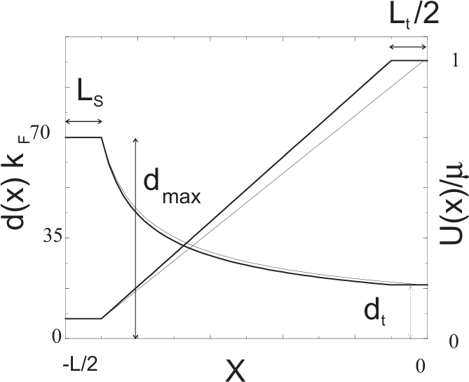
FIG. 2.: The shape of the model constriction that corresponds to a linear potential U(x), for two different $L_{t}$.

Obviously, the labels L and R refer to the location of the superconducting part with respect to the constriction.

The above forms shall be used as boundary conditions for Eq. (12).

III Model

The model constriction is depicted in FIG. 2. The constriction is symmetric. To simplify numerical calculations, we choose the shape of the boundaries in such a way that the effective one-dimensional potential $U(x)$ either remains constant of varies linearily. This choice has the advantage that the solutions of Eq. (12) can be readily expressed in terms of well-known Airy functions. The effective potential and the corresponding shape of the constriction, $d(x)$, are shown in FIG. 2.

The figure shows only half of the junction, the part in the negative $x$ direction. The constriction is long so that $Lk_{F}\gg 1$. The constriction is shallow so that the top of the potential $U_{max}$ for a transverse mode of interest almost matches Fermi energy, $U_{max}\approx\mu$. We thus define $\delta E\equiv\mu-U_{max}$, $|\delta E|\ll\mu$. This is achieved by a proper choice of the width $d_{t}$ in the middle of the constriction. An important parameter is also $L_{t}$, the length of the narrowest part of the constriction. The width reaches its maximum value $d_{max}$ at $|x|=(L-L_{t})/2$, which is at a distance $L_{s}$ from the superconductors.

Despite apparent simplicity of the model, it exhibits a variety of relevant energy scales. We list them going from bigger ones to smaller ones. The biggest scale is obviously the Fermi energy itself, $\mu$. Another important scale we obtain by considering electron reflection from one side of the top and disregarding existence of another side. Classically, the electron is fully transmitted at energies exceeding $U_{max}$ and fully reflected otherwise. Due to quantum effects, there is a smooth change from full reflection to full transmission that occurs within an energy interval $E_{c}$. There is a related length scale $x_{c}$ that corresponds to minimal electron wavelength. We estimate the typical length scale $x_{c}$ and the energy scale $E_{c}$ by equating potential and kinetic energy: $E_{c}\simeq(dU/dx)x_{c}\simeq\hbar^{2}/mx_{c}^{2}$. Let us note that by virtue of our model the potential derivative can be estimated as $dU/dx\simeq\mu/L$. By that we define an energy scale $E_{c}=0.03\mu(k_{F}L)^{-2/3}$ at which the reflection of electron waves from the top is changing to full transmission. The numerical coefficient is choosen in such a way that the reflection probability reaches $0.5$ at $E-U_{max}\approx E_{c}$. The energy dependence of the reflection probability is plotted in FIG. 3. The curve roughly behaves as $R\approx E_{c}/E$.

FIG. 3.: The reflection coefficient from the top as function of energy.

Three different energy scales arise from the interference of the electron waves either beyond or at the top of the potential. Beyond the top, the typical wavevector is of the order of $k_{F}$ and the interference condition reads $\delta kL\simeq\pi$. This gives $E_{i1}\simeq\hbar^{2}k_{F}\delta k/m\approx\pi\mu{(k_{F}L)}^{-1}$. The typical traversal time for this part of the system is of the order of $\hbar/E_{i1}$. The wavevector at the top is considerably smaller, $k_{top}\approx{(m\delta E)}^{\frac{1}{2}}/\hbar$. This may lead to much longer traversal times through the top of the constriction. Substituting $\delta E\simeq E_{c}$ we obtain the corresponding energy scale $E_{i2}=(2L/L_{t})(E_{c}/\mu)^{1/2}E_{i1}$, and $E_{i2}\ll E_{i1}$ if $L\simeq L_{t}$.

The third energy scale we obtain by estimating the energy counted from the top at which a few wavelengths match the length of the top, $k_{top}L_{t}\simeq 1$. This yields $E_{i3}\simeq\mu(k_{F}L_{t})^{-2}$. The same energy scale $E_{i3}$ determines when tunneling through the top becomes essential. We see that $E_{i2}\ll E_{c}$, at least if $L\simeq L_{t}$. Usual assumptions for adiabatic constrictions are such that $E_{i2}\simeq E_{c}$.[7] This makes our theory distinct from, for instance, Ref. [5].

The above analysis of our model captures the essential features of electron propagation in long shallow junctions and all qualitative results are actually model-independent.

We have performed numerical calculations for constrictions that have a length $L$ ranging from $10^{5}k^{-1}_{F}$ to $10^{6}k^{-1}_{F}$, and $d_{max}$ = $70k^{-1}_{F}$ at the SN boundaries. The width at the middle $d_{t}$ is chosen to vary between 17 and 28 $k^{-1}_{F}$ that assures that $U_{max}\approx\mu$ for the transverse mode $n=6$.

Using the Airy function solutions of Eq. (12), we estimate the errors involved in neglecting the terms in Eq. (7), which contain derivatives of $d(x)$. As far as the first derivative is concerned, looking at the second and third term in Eq. (7), we calculated the relative errors

$$\frac{d^{{}^{\prime}}(x)Ai^{{}^{\prime}}(x)}{(\mu-U(x))d(x)Ai(x)}\hskip 14.22636pt{\rm and}\hskip 14.22636pt\frac{d^{{}^{\prime}}(x)Bi^{{}^{\prime}}(x)}{(\mu-U(x))d(x)Bi(x)}$$ (25)

for the two Airy functions $Ai(x)$ and $Bi(x)$, for three $x$ values, at the beginning of the constriction, somewhere in the middle, and at the position where the narrowing has come to an end. Looking at the fourth term, and realizing that for our linear potential $U(x)=tx+c$ the relation $d^{{}^{\prime\prime}}d=3{d^{{}^{\prime}}}^{2}$ holds, we calculated the relative error

$$\frac{{\left(\frac{d^{{}^{\prime}}(x)}{d(x)}\right)}^{2}\left(\frac{n^{2}\pi^{2}}{12}+\frac{1}{2}\right)-\frac{d^{{}^{\prime\prime}}(x)}{2d(x)}}{\mu-U(x)}=\frac{\left(\frac{n^{2}{\pi}^{2}}{12}-1\right){\left(\frac{d^{{}^{\prime}}(x)}{d(x)}\right)}^{2}}{\mu-U(x)}$$ (26)

at the same positions as well. For the three points mentioned and for five different energies smaller than $|\Delta|$ the average error in the first derivative appeared to be smaller than $0.01\%$, and the error in the second derivative was even a factor of $10^{3}$ smaller. It could be concluded, that the omitted terms are really negligible.

IV Semiclassical Andreev states

Let us start by presenting a semiclassical picture of Andreev states in the simplest case where electrons and holes are either fully transmitted or fully reflected from the potential $U(x)$. We count energies of the states from the chemical potential. We denote $\delta E\equiv\mu-U_{max}$.

We assume no phase difference between superconductors. The Andreev state with positive energy $E$ is made of electron waves with energies $E$ and $-E$, those we call ”electrons” and ”holes” respectively. There may be three situations, depicted in FIG.4: I. Both electron and hole are fully transmitted through the constriction, $\delta E>0$ and $E<\delta E$. II. Both electron and hole are reflected from the top, $\delta E<0$ and $E<|\delta E|$. III. The electron is transmitted and the hole is reflected, $E>|\delta E|$. Since the potential $U(x)$ varies slowly, the quantized energies of Andreev states may be obtained from the Bohr-Sommerfeld quantization rule applied to Eq. (12).

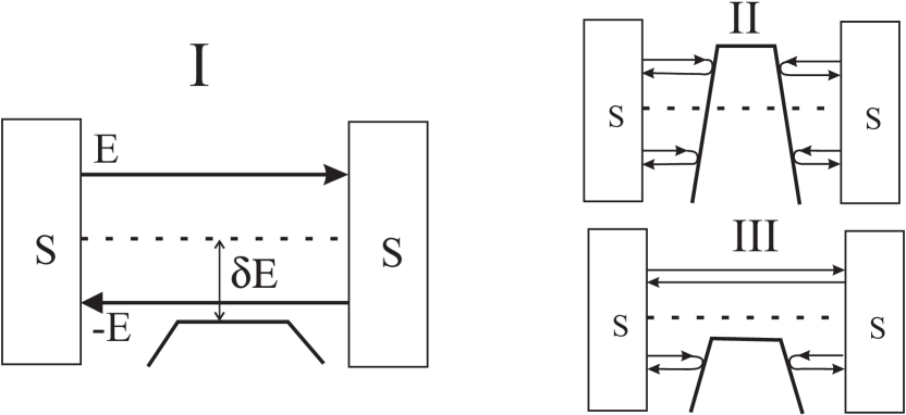
FIG. 4.: Three types of semiclassical Andreev states. The type III is specific for the absence of electron-hole symmetry.

The solutions of Eq. (12) can be written in the form

$$e^{i\int^{x}k_{+}(s)ds}\hskip 5.69054pt{\rm and}\hskip 5.69054pte^{i\int^{x}k_{-}(s)ds}$$ (27)

for the electron and hole part of $\phi_{n}(x)$ respectively, where $k_{\pm}=\sqrt{2m(\mu-U(x)\pm E)}/\hbar$. We begin our discussion with the case I. In this case, an electron travelling from left to the right builds up a phase of $\int_{-L/2}^{L/2}k_{+}(x)dx$. The electron undergoes Andreev reflection and returns as a hole, and the wave function gains the additional phase $\phi_{A}=\rm{acos}(E/\Delta)$, see Eqs. (15) and (21). The hole builds up a phase of $\int_{L/2}^{-L/2}k_{-}(x)dx$. After Andreev reflection at the left side, the particle has made a complete roundtrip. The quantization condition is that the phase gain is a mupliple of $2\pi$, that is

$$\int_{-L/2}^{L/2}(k_{+}(x)-k_{-}(x))dx+2\phi_{A}=2\pi n$$ (28)

Differentiating Eq. (28) with respect to $E$ gives an approximate relation for the energy difference between adjacent Andreev states,

$$E_{n+1}-E_{n}={2\pi\hbar}(T_{el}+T_{hole}+2\hbar\frac{\partial\phi_{A}}{\partial E})^{-1}$$ (29)

where we have introduced semiclassical times of travelling from the one interface to the other one, for electrons and holes respectively,

$$T_{\rm el}=\int_{-L/2}^{L/2}\frac{dx}{\sqrt{2(\mu-U(x)+E)/m}}\hskip 5.69054pt{\rm and}\hskip 5.69054ptT_{\rm hole}=\int_{-L/2}^{L/2}\frac{dx}{\sqrt{2(\mu-U(x)-E)/m}}.$$ (30)

and made use of semiclassical relation between the travelling time and the derivative of the quantummechanical phase with respect to the energy. If there are $many$ bound Andreev states, their typical spacing shall be small being compared to $\Delta$, so that $T_{el,hole}\gg\hbar/\Delta$. Since the derivative of the Andreev phase is of the order of $1/\Delta$, the second term in the right hand side of Eq. (29) can be disregarded and $E_{n+1}-E_{n}\approx 2\pi\hbar{(T_{el}+T_{hole})}^{-1}$ This suggests a presentation of our numerical results: we will plot the energy spacing times the travelling time as a function of the state energy. For the sake of symmetry we will use

$$\frac{1}{2\pi\hbar}(E_{n+1}-E_{n})\hskip 2.84526pt{\rm Av}\{T_{\rm el}+T_{\rm hole}\}\equiv\Theta,$$ (31)

where ${\rm Av}\{T_{\rm el}+T_{\rm hole}\}=\frac{1}{2}(T_{\rm el}(E_{n})+T_{\rm hole}(E_{n})+T_{\rm el}(E_{n+1})+T_{\rm hole}(E_{n+1}))$. The right hand side just defines the compact notation $\Theta$, and $\Theta\rightarrow 1$ in the classical limit. It is important to note that the Andreev states in this situation are degenerate. The state with electrons going to the right and holes going to the left has precisely the same energy as the state with electrons going to the left and holes going to the right. To be closer to our concrete model, let us introduce $T_{b}$, the travel time from one of the interfaces to the top, and $T_{t}$, the travel time through the top. The full traversal time for the case I is then $4T_{b}+2T_{t}$.

In case II the electron coming from the left is reflected from the top, gets back to the left interface, undergoes Andreev reflection, gets to the right as a hole, gets back and finally undergoes yet another Andreev reflection. The energy spacing is again given by the inverse of the time of semiclassical motion. This time is now $4T_{b}$. The Andreev states on the left side of the constriction do not overlap with the ones on the right side. This also leads to two-fold degeneracy of Andreev states for our symmetric setup.

In the case III the electron coming from the left passes the constriction and undergoes Andreev reflection on the right side. The resulting hole goes to the left, is reflected from the top and undergoes Andreev reflection on the right side again. This results in an electron going to the left that undergoes Andreev reflection on the left side. There are thus four Andreev reflections involved. The state encompasses the electron and hole waves that propagate in both directions. Therefore it is not degenerate. The travelling time is now $8T_{b}+2T_{t}$.

If $T_{t}\ll T_{b}$, the spacing of the states of the types I and II are evidently the same. For type III states, the travelling time is now approximately two times longer, which corresponds to a two times lesser energy spacing. However, there is no degeneracy in this case. This is why the number of states per energy interval remains approximately the same in all three cases. If $T_{t}\gg T_{b}$, there is a big spacing between type II states corresponding to energy scale $E_{i1}$. The spacing of the type I and type II states is much smaller.

Even a short glance at our numerical results proves that the picture based on the Eqs. (27) and (28) is oversimplified. In the following section we present a more sophisticated picture, which accounts for the oscillating phenomena, found from the full solution of the Bogoliubov equations (12).

V Qualitative results

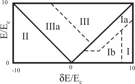
FIG. 5.: The parameter regions were different types of Andreev states occur. The reflection from the top causes interference that gives rise to electron, hole and irregular oscillations in the regions IIIa, Ia and Ib respectively.

Now we are in the position to present a concise summary of our qualitative results. Relevant parameters that determine the behaviour of the Andreev states are their energy $E$ and the shift $\delta E$ of the chemical potential with respect to the potential maximum. The superconducting gap $\Delta$ just determines the energy interval where Andreev states may be present, provided there are many states in this interval.

The parameter regions exhibiting distinct behavior of Andreev states are presented in FIG. 5. Two diagonal lines correspond to either electron or hole part of the state crossing the top of the potential relief. These lines separate the regions I, II and III discussed in the previous section. In these regions, the Andreev states are almost equally spaced, with the spacing being a slow function of energy. The energy scale of the spacing corresponds to ${\it min}(E_{i2},E_{i1})$. The semiclassical theory relates the spacing with the classical traveling time. From this one would conjecture a sharp crossover between the regions I, II, III, this presumably taking place in an energy interval of the order of several level spacings. This in fact corresponds to the situation described in Ref. [5].

The transitions between the regions I, II and III are much less trivial for a long shallow constriction described here. The reason for that is a strong reflection from the top of the constriction that takes place in a wide energy interval $\simeq E_{c}$ near the lines, see FIG. 3. The reflection takes place at two edges of the top. The interference between the reflected and transmitted waves disrupts a simple picture of semiclassical Andreev states.

This is why we have three more regions, IIIa, Ia, and Ib in the diagram. They are separated by dashed lines from their parent regions. Whereas the solid lines denote sharp transitions between the regions, the dashed lines correspond to smooth crossovers. For our concrete model, the crossovers are really very blurred, and the extra regions are difficult to separate from the parents. The reason for that is a slow decrease of the reflection coefficient with the energy, $R\approx E_{c}/E$. The crossovers may become sharper in a different model of a long shallow constriction. The regions would remain the same.

It is relatively easy to comprehend the situation in the region IIIa. There, the holes are completely reflected from the top and the transmitted and reflected waves do not interfere. They do interfere for electron components. This results in a regular modulation of spacings between Andreev states, which we call electron oscillations. We present in an Appendix a detailed theory of this effect. Here we give a final relation for ”energy spacing times travelling time” $\Theta(E)$, see Eq. (A13):

$$\Theta(E)=1+\frac{2T_{b}}{T_{t}+2T_{b}}\frac{\cos(2\phi_{b})\sqrt{R}-R}{1+R-2\cos(2\phi_{b})\sqrt{R}},$$ (32)

$R$ being the energy-dependent reflection coefficient from the edge of the constriction middle and $\phi_{b}$ being a linear function of energy, $\phi_{b}(E)={\rm const.}+\pi E/E_{i1}$. If $E_{i2}\ll E_{i1}$, each electron oscillation encompasses many Andreev states, of the order of $E_{i1}/E_{i2}$.

In the region Ia the situation is almost the opposite. Here, those are holes that are strongly reflected from the top. The electrons go at higher energy and are being transmitted much better. So one expects interference of holes only. We will call this phenomenon hole oscillations. Due to the slow decrease of the reflection coefficient mentioned above, the remaining interference of electrons is substantial. Therefore, the hole oscillations are not as regular as the electron ones. Also, the oscillation period is set by the inverse of the time for electrons to travel through the top, $T^{el}_{t}$. The ratio of $T^{h}_{t}/T^{el}_{t}$ is not parametrically big, so that the oscillation encompasses only few Andreev states. In our numerical results, we see alternating spacing of Andreev states in the region Ia.

In the region Ib both electrons and holes exhibit reflections, and the interference picture thus becomes complicated and at best quasi-periodic. We will call this irregular oscillations. The visible quasi-period is $E_{i1}$ again. It arises as a result of interference of two reflections, one for the electron component and another for the hole one. These reflections are coupled by an Andreev process. One would not see such period in the interference picture of a normal electron.

All these three types of oscillations are seen in our numerical results. Another effect of the reflection is that the degeneracy between Andreev states is lifted. For our symmetric setup, the Andreev states can be either even or odd, that is, symmetric or antisymmetric with respect to $x\rightarrow-x$.

VI Numerical results

For numerics, we choose the transverse dimensions in such a way that only six modes can pass the constriction. For the sixth mode, the Fermi level matches the potential in the middle of the constriction and $|\delta E|\ll\mu$. We note that from now on $\Delta$ is chosen to be a real constant, since we assume no phase difference between the superconductors. If $\delta E=0$ only the electron can pass the constriction. As soon as $\delta E<-\Delta$ no transmission occurs for the waves forming Andreev states. Since the interesting phenomena occur for the sixth mode and for not too big values of $\delta E/\Delta$, we will show results for $\delta E/\Delta$ taking values 10, 2, 1, 0.5, 0, -0.5, -1 and -2 only.

Most calculations were done using a gap value of $4\times 10^{-5}\mu$, which is sufficiently small to achieve the semiclassical limit under investigation.

FIG. 6.: $\Theta$ as defined by Eq. (31) versus the relative Andreev bound state energy $E/\Delta$, for a system length $Lk_{F}=7\times 10^{4}$. The first five modes support just one state each, while for the sixth mode the number of states is seven. Both electrons and holes traverse the system.

In order to get a feeling for the system properties we first show the Andreev states spectrum for all modes and the two system lengths $L=7\times 10^{4}k_{F}^{-1}$ and $2.1\times 10^{5}k_{F}^{-1}$ in the FIGs. 6 and 7 respectively. For both cases $\delta E=10\Delta$, so both components of an Andreev state can transit the system. The system lengths are such that the first five modes for $L=7\times 10^{4}k_{F}^{-1}$ support one bound state each, while for the three times longer system two bound bound states are found. The energies of these states are plotted with the circles.

The energy separation for the lower modes is approximately $E_{i1}$, which is of the order of $\Delta$ choosen. The wavefunctions of corresponding states easily pass the middle part of the constriction and their energies do not depend on $\delta E$, being very large for these states. Because they do not exhibit any interesting behavior we do not pay further attention to the first five modes. We just mention, that in all results to be displayed the Andreev approximation is made at the two SN interfaces. In the exact treatment the degeneracy of the two Andreev states with the two opposite propagation directions is lifted, and one ends up with two standing waves, a symmetric and an antisymmetric one. We calculated the exact energies for the five states depicted in FIG. 6 by filled circles, and found a splitting of the order of $10^{-10}\mu$, which is negligible indeed.

More states are found for the sixth mode. Since they traverse the top, their energy separation is determined by $E_{i2}\gg E_{i1}$ rather than $E_{i1}$. We begin the discussion with FIG. 7. There are 20 Andreev states, as can be seen in the figure. Both the odd and even states are shown, the corresponding $\Theta$ values being connected by broken and solid lines respectively. We see that the $\Theta$ values are close to 1, which proves the validity of the semiclassical treatment. So we concentrate on the deviations from 1. The energy distance from the top of the potential $\delta E\approx 47E_{c}$. Although the waves are still well transmitted, the reflection probability at the narrow part of the constriction becomes already appreciable (2%).

This leads to two visible phenomena. First, the two states corresponding to two travelling waves propagating in opposite directions are mixed by reflection. By that the even and odd states have different energies. The stars in the figure indicate the result for an average energy, which corresponds to two degenerate states found after neglect of reflection at the constriction. The actual calculation in which only propagation to the right is allowed can be achieved by omitting the contribution of the wave propagating to the left in the normal metallic part at the left SN interface. The corresponding $\Theta$ values are somewhat smaller than 1, but they lie at a stable height, in agreement with the estimate based on the forms (27), in which any reflection is not accounted for. The deviation of the stars from the lines is the measure of the effect.

FIG. 7.: The same as in FIG. 6, but for a three times longer system length $Lk_{F}=2.1\times 10^{5}$. The reflection has increased resulting in bigger amplitude of irregular oscillations of Andreev spacing. For the first five modes two states are found for each mode, while for the sixth mode the number of states is twenty.

Second, the interference between the reflected waves leads to irregular dependence of $\Theta$ on energy, as discussed in section V. The amplitude of these irregular oscillations is small corresponding to the small reflection coefficient.

Both effects are better visible in FIG. 6 where the constriction is shorter and only seven states are seen. They are displayed by four triangles and three squares. However, this is not the main difference between the figures. The energy distance $\delta E$ becomes $\approx 23E_{c}$, which corresponds to a reflection coefficient of the order of 4%. The energy difference between the odd and even states becomes considerable, even such, that the highest state, a symmetric solution, does no longer have its antisymmetric counterpart. This would have got an energy $E>\Delta$, while bound states are only found below the gap. The irregular oscillations are increased in amplitude.

FIG. 8.: The same as in FIG. 6, but only for mode 6 states. Irregular oscillations in the region Ib. The hole branch of the Andreev states lies always an energy higher than the gap energy above the barrier in the middle. We show results for two system lengths $2.1\times 10^{5}$ and $7\times 10^{5}$, which give 38 and 119 bound states respectively. The reflection coefficient varies between 0.05 and 0.1. The typical quaisiperiod is of the order of $E_{i1}$.

FIG. 9.: For $\delta E=\Delta$ the bound states near $\Delta$ have a hole component touching the top of the potential. Strong reflection of these holes give rise to hole oscillations above $\approx 0.7\Delta$. Two gap values correspond to 66 and 95 Andreev states.

Results for $\delta E=2\Delta$ are shown in FIG. 8. In addition to the results for the system length $L=2.1\times 10^{5}$ the even states are shown for the larger length of $L=7\times 10^{5}$. The number of states has increased to 119, and the oscillation frequency has increased as well. The two choices of $L$ correspond to $\delta E/E_{c}\approx 10$ and $\delta E/E_{c}\approx 21$. The irregular oscillations are bigger in the first case, which corresponds to the bigger reflection. Due to larger number of states, one can see already a typical (quasi)period. The biggest interference scale $E_{i1}$ is $0.37\Delta$ and $0.11\Delta$ respectively. We see a good correspondence between this scale and the quasiperiod.

The next figure, FIG. 9, presents the results for $\delta E=\Delta$, when Andreev states extend till the energy at which holes are reflected completely. We observe a new type of oscillations at energies $>0.6\Delta$. At these energies, the holes are reflected more effectively than electrons. So that the oscillations are determined mostly by their interference. The two choices of $\Delta$ correspond to $\delta E/E_{c}=4.75$ and $\delta E/E_{c}=9.5$.

The most interesting figure is probably FIG. 10, which displays $\delta E=0.5\Delta$ results. The parameter choice corresponds to $\delta E\approx 3.3E_{c}$. All three types of oscillations can be simultaneously seen there. The oscillations are irregular till $E\approx 0.3\Delta$ and they cross over to hole oscillations at higher energy. At $E=0.5\Delta$ the holes are completely reflected, and the interference picture is determined solely by electrons. The transition is sharp indeed, the width being of the order $E_{i3}=2\times 10^{-5}\Delta$. These electron oscillations are very regular. Their period is determined by $E_{i1}=0.22\Delta$, each oscillation encompassing about 10 Andreev states. There is a striking contrast between the electron and hole oscillations, the latter being much less regular. The point is that the hole oscillations are disrupted by residual interference of electrons and the electron oscillations are not, since holes do not penetrate the middle of the constriction and do not interfere.

FIG. 10.: At $\delta E=0.5\Delta$ the hole component is completely reflected in the middle of the constriction at $E>0.5\Delta$. All three types of oscillations are seen simultaneously in this plot.

The electron oscillations throughout the full range of Andreev states are presented in FIG. 11. Here the width of the constriction is chosen in such a way, that $U(x)$ in the middle coincides with the Fermi energy and $\delta E=0$. All hole waves are reflected completely from the middle of the constriction, while all electron waves still can pass. The parameters correspond to $\Delta/E_{c}\approx 4.5$ for the solid curve and $\Delta/E_{c}\approx 19$ for the dashed one. This means that the reflection coefficient from the top varies from $1$ to $\approx 0.2$ or $\approx 0.05$ respectively. This affects the oscillation amplitude. In FIG. 11 one indeed sees that the position of the dips moves upwards with the energy, most clearly for the larger gap value.

FIG. 11.: The electron oscillations through the whole energy range. The hole component is completely reflected for all energies. Each oscillation encompasses about ten states. Circles and stars represent the states for a very short middle of the constriction and for the smaller gap value of $\Delta=4\times 10^{-5}\mu$. Note the correspondence of their positions and the oscillation dips.

The spacing between the states and the oscillation period are determined by energy scales $E_{i2}$ and $E_{i1}$ respectively. This is why for four times larger gap four times more states and oscillations are found.

We remind that up to now all calculations were done with the length of a flat part in the middle equal to $10\%$ of the system length, $L_{t}=0.1\ L$. We also show in FIG. 11 the results for much shorter flat part length $L_{t}=10^{-3}L$. Six states are found, three odd states and three even states. For these parameters, the constriction middle is so short that $E_{i2}\gg E_{i1}$, and the spacing is of the order of $E_{i1}\approx 0.37\Delta$. This is why the Andreev states for the short top match the oscillations of Andreev states for the long top. The matching is not perfect. The reason for that is the tunneling of the holes through the top, which becomes considerable for the short top ($E_{i3}=0.5\Delta$).

FIG. 12.: In this case, $E=0.5\Delta$ separates regions II and III b. The Andreev states in the region II are localized near the superconductors and do not go through the middle of the constriction. Note the correspondence between the spacing of the states at low energy and oscillation period at higher energy.

The following results are for parameter range $\delta E<0$ where holes are completely reflected from the top. FIG. 12, with $\delta E=-\frac{1}{2}\Delta$, is a counterpart of FIG.10, with $\delta E=\frac{1}{2}\Delta$. This means that the electrons are completely reflected at $E<\frac{1}{2}\Delta$ and transmitted at higher energies. By that the oscillations arise for the higher energies only, which is clearly seen in the figure. For $E<\frac{1}{2}\Delta$ the two parts of the constriction are in fact not connected. The Andreev states calculated are doubly degenerate, with one state resting in the left part of the constriction and the other state in the right part. The spacing between these states is of the order of $E_{i1}$ for both values of $\Delta$. Again, this scale sets the oscillation period for the states above $\Delta/2$, whereas their spacing is determined by much smaller energy scale $E_{i2}$. Two values of $\Delta$ correspond to $\Delta/E_{c}\approx 4.5$ and $\Delta/E_{c}\approx 19$.

FIG. 13.: Localized Andreev states in the region II. Their spacing is a smooth function of energy. Their energies hardly depend on the position of the chemical potential with respect to the maximum of the potential.

The results depicted in FIG. 13 correspond to $\delta E=-\Delta$ and $\delta E=-2\Delta$. So we have the space separation of Andreev states in the whole energy interval. No interference occurs, and the spacing $\Theta$ is a smooth function of energy. The differences between $\delta E=-\Delta$ and $\delta E=-2\Delta$ are small. For the smaller gap value the number of states is of the same order as the degenerate states for mode 6 in FIG. 6. The Andreev levels hardly depend on $\delta E$, since they never reach the middle of the constriction and do not experience the potential over there.

VII Conclusions and prospects

In conclusion, we present here a theory of Andreev states for a shallow long adiabatic constriction. The system differs from traditional models of S-N-S junctions by the absence of electron-hole symmetry and exhibits at least four disctict energy scales that determine the interference of the components of Andreev states. Such constrictions can be possibly realized in semiconductor heterostructures.

We have started with a completely semiclassical approach to the states and reached in the first approximation a good agreemement with exact solutions of Bogoliubov equations. On the top of this, the exact Andreev levels may exhibit three distinct types of oscillating behavoir. These oscillations arise from interference of the transmitted and reflected waves in the middle of the constriction. We have extended the semiclassical theory to account for this interference and were able to reach quantitative agreement with numerical results.

In this paper, we assumed no phase difference between the superconductors. It would be interesting to calculate the Andreev states in the presence of such phase difference and finally find the supercurrent in the structure. It is already clear that the supercurrent would exhibit an interesting dependence on controllable system parameters, in particular, on $\delta E$. This makes such calculation interesting in view of possible experiments.

A Interference of Andreev states

FIG. 14.: Schematical picture of our constriction, including the paths of the electron and hole branches of the Andreev bound states. The Fermi energy coincides with the flat part of the potential at the constriction. In the quasiclassical derivation reflections of the electron wave are accounted for which are taken to occur at the the entrance and exit of the constriction. Reflection 1 occurs at the point A, which coincides spatially with point D, and reflection 2 occurs at point B (or C).

The shape of the oscillations can be understood in quasiclassical terms if the interference of the waves is taken into account. The configuration of the system and the parameters used are shown in FIG. 14.

To evaluate the quantization condition, we consider the amplitude of the wave that starts propagating from point X, goes all the way through the constriction and gets back to the same point. The starting point can be chosen arbitrarily. Each part of the trajectory contributes a factor of the form $e^{i\phi}$ to the amplitude. The phases $\phi_{1}$, $\phi_{2}$ and $\phi_{4}$ are shown in the figure, $\phi_{3}$ is the propagation phase from B to C, and $\phi_{5}$ is the phase from D to X. If there is no reflection at A, B, C and D

$${\rm Amplitude}=e^{i\phi_{1}}e^{i\phi_{2}}e^{i\phi_{3}}e^{i\phi_{4}}e^{i\phi_{5}}=1,$$ (A1)

in which the second equality is the condition for an Andreev bound state. This quantization condition can be written as

$$\phi_{1}+\phi_{2}+\phi_{3}+\phi_{4}+\phi_{5}=2\pi n$$ (A2)

Using the symmetries

$$\phi_{1}+\phi_{5}=\phi_{3}\equiv 2\phi_{b}\hskip 11.38109pt{\rm and}\hskip 11.38109pt\phi_{2}=\phi_{4}\equiv\phi_{t}$$ (A3)

one can write down the equality

$$2\pi\hbar\frac{{\rm d}n}{{\rm d}E}=2T_{t}+4T_{b},$$ (A4)

where $T_{t}$ is the time for the classical motion between the points A and B, and $T_{b}$ is the time it takes to get from the interface to the constriction top. Here we made use of the quasiclassical relation between the phase and the time of the classical motion $\hbar\frac{{\rm d}\phi}{{\rm d}E}=T$. Eq. (A4) can be considered as a slight generalization of Eq. (28).

Now we extend the analysis by assuming the possibility of relections at the points A, B, C and D. For each point four coefficients are to be defined, namely $t_{LR}$ and $t_{RL}$ for transmission from left to right and from right to left respectively, and $r_{LR}$ and $r_{RL}$, similarly, for reflection. By summing up all possible ways of propagation, from the point X to the right and back to that point coming from the left, and accounting for all reflections and transmissions one arrives at

$${\rm Amplitude}=e^{i(\phi_{1}+\phi_{5})}[r_{LR}^{(1)}+\frac{t_{LR}^{(1)}t_{RL}^{(1)}{\rm A}_{AD}}{1-r_{RL}^{(1)}{\rm A}_{AD}}]=1,$$ (A5)

in which the second equality is the quantization condition. The quantity ${\rm A}_{AD}$ is the amplitude to get from A to D and is given by

$${\rm A}_{AD}=e^{i(\phi_{2}+\phi_{4})}[r_{LR}^{(2)}+\frac{t_{LR}^{(2)}t_{RL}^{(2)}e^{i\phi_{3}}}{1-r_{RL}^{(2)}e^{i\phi_{3}}}].$$ (A6)

Again using the phases $\phi_{b}$ and $\phi_{t}$, solving Eq. (A5) for ${\rm A}_{AD}$, and using Eq. (A6), one obtains the symmetric form

$$e^{2i\phi_{t}}\hskip 5.69054pt\frac{z^{(1)}e^{i2\phi_{b}}+r_{RL}^{(1)}}{1-e^{i2\phi_{b}}r_{LR}^{(1)}}\hskip 5.69054pt\frac{z^{(2)}e^{i2\phi_{b}}+r_{LR}^{(2)}}{1-e^{i2\phi_{N}}r_{RL}^{(2)}}=1,$$ (A7)

in which $z^{(1)}$ and $z^{(2)}$ are defined by

$$z^{(1,2)}\equiv t_{LR}^{(1,2)}t_{RL}^{(1,2)}-r_{LR}^{(1,2)}r_{RL}^{(1,2)}.$$ (A8)

We now study the general expression (A7) using simplifying assumptions. If we disregard scattering phases and their energy dependence we can write

$$r_{LR}^{(1)}=r_{LR}^{(2)}=r_{RL}^{(1)}=r_{LR}^{(2)}=\sqrt{R},$$ (A9)

$R$ being the reflection coefficient. By that we find, that $z^{(1,2)}=-1$ and the quantization condition (A7) becomes

$$e^{2i(\phi_{t}+2\phi_{b})}{\left(\frac{1-e^{-i2\phi_{b}}\sqrt{R}}{1-e^{i2\phi_{b}}\sqrt{R}}\right)}^{2}=1,$$ (A10)

which is equivalent to

$$2(\phi_{t}+2\phi_{b})+4\hskip 2.84526pt{\rm atan}\left(\frac{\sin(2\phi_{b})\sqrt{R}}{1-\cos(2\phi_{b})\sqrt{R}}\right)=2\pi n.$$ (A11)

For the energy derivative this gives

$$2\pi\hbar\frac{{\rm d}n}{{\rm d}E}=2T_{t}+4T_{b}+4T_{b}\frac{\cos(2\phi_{b})\sqrt{R}-R}{1+R-2\cos(2\phi_{b})\sqrt{R}}.$$ (A12)

We rewrite this using our definition of $\Theta$ and obtain the desired expression, see Eq. (32),

$$\Theta(E)=1+\frac{2T_{b}}{T_{t}+2T_{b}}\frac{\cos(2\phi_{b})\sqrt{R}-R}{1+R-2\cos(2\phi_{b})\sqrt{R}}$$ (A13)

If there are no reflections, $\Theta$ is equal to 1. If reflections are accounted for, Eq. (A13) implies, that for $R\ll 1$ small modulations below the value of 1 are found in plotting the quantity $\delta E(T_{t}+2T_{b})/\pi$ as a function of $E$ or $E/\Delta$. If $R\simeq 1$ periodic dips below the value of 1 are coming out, completely in agreement of the structure of FIG. 11. For a constant $R$ the dips lie at equal height. In reality $R$ is energy dependent at $E\simeq E_{c}$ and decreases with increasing energy. Recalling the definition of $\phi_{b},\phi_{t}$, we see that the spacing is determined by the energy scale $E_{i2}$ (provided $E\simeq E_{c}$) and the oscillation period is determined by the bigger energy scale $E_{i1}$.

Similar consideration can be performed for hole oscillations in the region Ia. This results in oscillations with a period determined by difference of phases accumulated respectively by electrons and holes during their travel though the middle of the constriction.

The irregular oscillations in the region Ib can be also quantified along these lines. However, here the reflection coefficients for the electron and hole wave are different, and different phase differences are accumulated by electrons and holes in the constriction middle and beyond. The typical quasiperiod is determined by the phase $\phi_{b}$, that varies with energy in a slowest way.

REFERENCES

- [1] A. F. Andreev, Sov. Phys. JETP 19, 1228 (1964); ibid., 24, 1019 (1967).
- [2] A. I. Larkin and Yu. V. Ovchinninkov, Sov. Phys. JETP 41, 960 (1975).
- [3] Yu. V. Nazarov, Phys. Rev.Lett. 73, 1420 (1994).
- [4] A. Lodder and Yu. V. Nazarov, Phys. Rev. B 58, 5783 (1998).
- [5] N. M. Chtchelkatchev, G. B. Lesovik, and G. Blatter Phys. Rev. B 62, 3559 (2000).
- [6] R.Kümmel, Phys. Rev. B 10, 2812 (1974); O. Ŝipr and B.L. Györffy, J. Phys.: Condensed Matter 8, 169 (1996).
- [7] L.I. Glazman, G.B. Lesovik, D.E. Khmel nitskii, and R.I. Shekhter, Pis ma Zh. Eksp. Teor. Fiz. 48, 218 (1988) (JETP Lett. 48, 238 (1988)).