Decoherence and dephasing in coupled Josephson-junction qubits

Abstract

We investigate the decoherence and dephasing of two coupled Josephson qubits. With the interaction between the qubits being generated by current-current correlations, two different situations in which the qubits are coupled to the same bath, or to two independent baths, are considered. Upon focussing on dissipation being caused by the fluctuations of voltage sources, the relaxation and dephasing rates are explicitly evaluated. Analytical and numerical results for the coupled qubits dynamics are provided.

, ,

1 Introduction

Nano-electronic devices have recently attracted much interest as possible candidates for the implementation of quantum computers. In fact, in contrast to ion traps [1] and NMR systems [2], nano-electronic devices are easily embedded in an electronic circuit, and can be scaled up to large number of quantum bits (qubits) and quantum gates. Ultra small quantum dots with discrete levels, and in particular spin degrees of freedom embedded in nano-scale structured materials have been proposed [3]. However, these systems are difficult to fabricate in a controlled way. More suitable candidates are Josephson contact systems, where the coherence of the superconducting state can be exploited, and which can be fabricated by well established litographic methods. Macroscopic flux states in a SQUID have been proposed as basic quantum bits [4]. Spectroscopy experiments of the flux qubit spectrum have recently been performed [5].

In this work we consider the alternative design which uses the charge in low-capacitance junctions as quantum degree of freedom [6, 7]. The logical states of the qubit are then macroscopic states differing by one Cooper pair charge. In a recent experiment Nakamura et al. have observed time-resolved coherent oscillations in such a Josephson junction set-up [8]. Several possible realizations have been by now discussed [7, 9, 10]. The set up we consider is discussed in Section 2, and it follows the design proposed in [10]. In particular, single bit and two-bit operations may be performed by applying a sequence of suitably tailored gate voltages.

Quantum computation requires a phase coherent time evolution. Hence, it is of prominent importance to deal with systems possessing long intrinsic phase coherence times, and to minimize possible external sources for dephasing [11]. Moreover, crucial for quantum computation is the ability to perform calculations with single as well as with coupled qubits. Previous works analyzed only dephasing times of single qubits [12], or gave an estimate for $N$ uncorrelated qubits [6]. Only a few previous works investigated the dynamics of coupled spins embedded in a thermal environment [13]. In this work we analyze the influence of dissipation and of thermal quantum fluctuations on the coherent evolution of two coupled qubits. We distinguish between two configurations: In the first one the two qubits are dephased by the same thermal bath. In the second one each qubit is coupled to its own environment. The general characteristics will be the theme of Section 3, where the phase coherence time and the decoherence rate will be explicitly evaluated for the two different environmental configurations. In Section 4 we provide analytical and numerical results for the population dynamics, when dissipation is dominated by fluctuations of the voltage sources. Finally, in Section 5 we draw some conclusions.

2 Josephson Junction Qubits

2.1 The Josephson-junction qubit

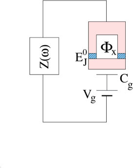
Figure 1: Charge qubit with Josephson coupling controlled by an external field $\Phi_{X}$ threading the dc-SQUID. The dissipative influence originating by voltage fluctuations are captured by an impedence $Z(\omega)$.

In the following we briefly discuss the design for tunable Josephson charge qubits following [7, 10]. It allows to manipulate the qubits parameters independently. The system consists of a tunable Cooper pair box, where a small superconducting island is connected to two tunnel junctions embedded in the two arms of a SQUID loop threaded by a flux $\Phi_{X}$, cf. Fig. 1. The junctions are supposed to be identical and are characterized by a capacitance $C^{0}_{J}$ and coupling energy $E_{J}^{0}$. In this situation, an ideal voltage source $V_{g}$ is connected to the system via a gate capacitor $C_{g}$. If the self-inductance of the SQUID is low, the two junctions effectively behave as a single junction being characterized by the effective capacitance $C_{J}=2C^{0}_{J}$, and by the tunable Josephson energy

$$E_{J}(\Phi_{X})=2E_{J}^{0}\cos(\pi\Phi_{X}/\Phi_{0})\;,$$ (1)

where $\Phi_{0}=h/2e$ is the flux quantum. Then, the charging energy of the superconducting island is characterized by the scale $E_{C}=e^{2}/(2C_{g}+2C_{J})$. In the following we consider the situation where the superconducting energy gap is the largest energy in the problem. Then only Cooper pairs tunnel through the superconducting junctions. In the regime $E_{J}\ll E_{C}$ a convenient basis is formed by the charge states parametrizing the number $n$ of Cooper pairs on the island. In this situation the dimensionless gate charge $n_{g}=C_{g}V_{g}/(2e)$ acts as a control field. For values of $n_{g}$ close to a half integer two adjacent Cooper pair states become close to each other. We concentrate on the voltage interval near a degeneracy point where two charge states, e.g. $n=0$ and $n=1$ play a role, while higher charge states, having much higher energy can be ignored. Hence, in the absence of dissipation, the system effectively reduces to a two-state system being described by the Hamiltonian

$$H_{\rm qb}=-\frac{1}{2}E_{z}(n_{g})\sigma_{z}-\frac{1}{2}E_{J}(\Phi_{X})\sigma_{x}\;,$$ (2)

where the $\sigma$’s are Pauli spin matrices, and $E_{z}=4E_{C}(2n_{g}-1)$ is controlled by the gate voltage. In this representation the charge states $n=0$ and $n=1$ correspond to the vectors $|\downarrow\rangle$ and $|\uparrow\rangle$ respectively. They are eigenstates of $\sigma_{z}$ with eigenvalues $-1$ and $1$, respectively. Hence, for a qubit being prepared in one of the eigenstates of $\sigma_{z}$, quantum coherent oscillations with frequency $E_{\rm qb}/\hbar$, with

$$E_{\rm qb}:=\sqrt{E_{z}^{2}+E_{J}^{2}}\;,$$ (3)

occur.

2.2 The electromagnetic environment

An ideal quantum system preserves quantum coherence, i.e., its time evolution is determined by deterministic reversible unitary transformations. In reality, any physical quantum system is subject to various disturbing factors which act in destroying the phase coherence. The concept of quantum computation heavily relies on the possibility of realizing quasi-ideal systems. Hence, it is crucial to investigate the effects of the environment on the qubits, and to understand how the environment induced dephasing can be minimized. It should also be realized that coherent quantum manipulations of the qubits are still possible if the dephasing time is finite but not too short. In fact, the quantum error-correction techniques [15] allow to correct errors if they do not occur too often.

In a charge Josephson qubit, the system is sensitive to the electromagnetic fluctuations in the external circuit and in the substrate, and to background charge fluctuations. We start by considering here the dissipative effects which arise from the fluctuations of the voltage sources. The equivalent circuit of a qubit coupled to an impedence $Z(\omega)$ is shown in Fig. 1. When $Z(\omega)$ is embedded into the circuit (with $E_{J}=0$), the voltage fluctuations between the terminals of $Z(\omega)$ are characterized by the equilibrium correlation function [6, 12]

$$\langle\delta V(t)\delta V(0)\rangle$$ (4)

$$= \frac{1}{\pi}\int_{0}^{\infty}d\omega{\rm Re}\{Z_{t}(\omega)\}\hbar\omega\left(\coth\left(\frac{\hbar\omega}{2k_{\rm B}T}\right)\cos(\omega t)-i\sin(\omega t)\right)\;.$$

Here $Z_{t}(\omega):=[i\omega C_{t}+Z^{-1}(\omega)]^{-1}$, with $C_{t}^{-1}=C_{J}^{-1}+C_{g}^{-1}$, is the total impedence between the terminals. Following [17] we model the dissipative influence of $Z_{t}(\omega)$ as resulting from a bath of harmonic oscillators described by the Hamiltonian

$$H_{\rm B}=\sum_{i}\left[\frac{p^{2}_{i}}{2m_{i}}+\frac{m_{i}\omega^{2}_{i}x_{i}^{2}}{2}\right]\;.$$ (5)

It is assumed that the voltage between the terminals of $Z_{t}(\omega)$ is given by $\delta V=\sum_{i}\lambda_{i}x_{i}$, and the spectral density $G(\omega):=\frac{\pi}{2}\sum_{i}\frac{\lambda_{i}^{2}}{m_{i}\omega_{i}}\delta(\omega-\omega_{i})$ is chosen to reproduce the fluctuations spectrum (4), i.e., $G(\omega)=\omega{\rm Re}Z_{t}(\omega)$. Thus, embedding the element $Z(\omega)$ in the qubit circuit one arrives, in the two-state approximation, to the spin-boson Hamiltonian [6]

$$H_{\rm SB}=H_{\rm qb}+H_{\rm B}+\frac{1}{2}\sigma_{z}X\;,$$ (6)

where $X:=2e(C_{t}/C_{J})\delta V$ describes the coupling to the bath. In the following we concentrate on the fluctuations due to an Ohmic resistor $Z(\omega)=R$. It is convenient to introduce the spectrum $J_{V}(\omega):=4e^{2}(C_{t}/C_{J})^{2}G(\omega)$. For an Ohmic resistor it assumes the form $J_{V}(\omega)=2\pi\hbar\alpha\omega$ which is linear at low frequencies up to some cut-off $\omega_{c}=(RC_{t})^{-1}$. The dimensionless parameter $\alpha$ which characterizes the strength of the dissipative effects reads

$$\alpha=\frac{4R}{R_{\rm K}}\left(\frac{C_{t}}{C_{J}}\right)^{2}\;,$$ (7)

where $R_{\rm K}=h/e^{2}\approx 25.8$k$\Omega$ is the quantum resistance. Hence, in order to make dissipation small one has to use a voltage source with very low resistance, and choose the gate capacitance $C_{g}\approx C_{t}\ll C_{J}$ as small as possible. For a typical resistance $R\approx 50\Omega$ one has $\alpha\approx 10^{-2}(C_{g}/C_{J})^{2}$. Upon choosing $C_{J}\approx 100aF$ and $C_{g}\approx 1aF$ one can reach coupling parameters as small as $\alpha\approx 10^{-6}$.

A similar line of reasoning can be performed to include also the effect of $1/f$ noise due to background charges [16]. It is found that the effect of the background charges can be mapped into that of a harmonic oscillator bath with a spectrum that may have a simple behavior $J_{1/f}(\omega)\propto K/\omega$. Usually, such fluctuations occur on a longer time scale than the voltage fluctuations. They also limit the coherence of the system. However in our charge qubit set-up dissipation is dominated by voltage flucutuations. In the following we shall mainly consider the effects of a harmonic bath being characterized by the Ohmic spectral density $J_{V}(\omega)$. However, how to include $1/f$ noise in our formalism will be discussed in the next Section .

Finally, one can consider the effects of the fluctuations of the externally supplied flux through the SQUID loop of the charge qubit. These fluctuations couple to the qubit variable $\sigma_{x}$. We relate them to an effective impedence $R_{I}$, assumed to be real, of the current circuit. At typical high frequencies of the qubit’s operation this resistance is of the order of the vacuum impedence $R_{I}\approx 100\Omega$. This yields for the dimensionless coupling constant [6]

$$\alpha_{x}=\frac{R_{\rm K}}{R_{I}}\left(\frac{M}{\Phi_{0}}\frac{\partial E_{J}(\Phi_{X})}{\partial\Phi_{X}}\right)^{2}\;,$$ (8)

with $M$ being the mutual inductance. For $M\approx 0.01$nH and $E_{J}^{0}\approx 0.1$K one obtains $\alpha_{x}\approx 10^{-8}$. Thus, these latter fluctuations seem not to be dominant, and will be neglected in the following treatment. They can however be easily included in our formalism, as we shall discuss in Section 3.

2.3 Coupled qubits

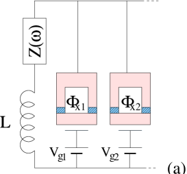
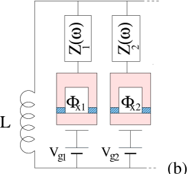
Figure 2: A register of many charge qubits coupled to a common inductor $L$. In case a) the qubits are subject to a common dissipative environment, while in configuration b) each qubit is coupled to its own oscillator bath.

For quantum computation pairs of qubits have to be coupled in a controlled way. In the scheme proposed in Fig. 2 all qubits are coupled by one mutual inductor $L$. For $L=0$ the system reduces to a series of uncoupled qubits, while they are coupled strongly when $L\to\infty$. Hence, for finite $L$, the total Hamiltonian of this system consists of $N$ qubits contributions as in (2), and of an oscillator resulting from the inductance and the total capacitance $NC_{t}$, with $C_{t}^{-1}=C_{J}^{-1}+C_{g}^{-1}$, of all qubits. The voltage oscillations in the $LC_{t}$ circuit affect all the qubits equally. They induce a phase shift $2\pi\varphi=2\pi\frac{C_{t}}{C_{J}}\frac{\Phi}{\Phi_{0}}$ of the phase variables $\Theta_{i}$ conjugated to the Cooper pair number $n_{i}$ of the $i$-th qubit. Here $\Phi$ denotes the flux in the mutual inductor, and $\Phi_{0}=h/2e$ is the flux quantum. In the following the parameters are chosen such that the oscillator remains in the ground state for all relevant operation frequencies, i.e., $E_{C},E_{J}\ll\hbar\omega_{L}$, where $\omega_{L}=(NLC_{t})^{-1/2}$ is the characterisitic oscillator frequency. Moreover, we assume that fluctuations of the phase shift $\varphi$ are small compared to unit, i.e., $\frac{C_{t}}{C_{J}}\sqrt{\langle\Phi^{2}\rangle}\ll\Phi_{0}$. Since $\langle\Phi^{2}\rangle/L\approx\hbar\omega_{L}/2$ this condition imposes only weak constraint on the parameters. Then, although the $LC_{t}$ oscillator remains in its ground state, it provides an effective coupling between the qubits. It reads [10]

$$H_{\rm int}=-\sum_{i<j}\frac{E_{J}(\Phi_{Xi})E_{J}(\Phi_{Xj})}{E_{L}}\sigma_{y}^{(i)}\sigma_{y}^{(j)}\;,$$ (9)

with the energy scale

$$E_{L}=\left(\frac{C_{J}}{C_{g}}\right)^{2}\frac{\Phi_{0}^{2}}{\pi^{2}L}\;,$$ (10)

while $E_{J}^{i}=E_{J}(\Phi_{Xi})$ are the effective Josephson energies of the qubits, controlled by the external flux. This coupling energy can be easily understood as the magnetic energy of the current in the inductor, where the current is the sum of the contributions from the qubits with non zero Josephson coupling, $I_{i}\propto E_{J}^{i}\sigma_{y}^{(i)}$. Noticeably the strength of the interaction does not depend on the number of qubits in the system. However, the frequency $\omega_{L}$ of the oscillator scales with $1/\sqrt{N}$. This limits the allowed number of qubits in the system, since this frequency should not drop below typical eigenfrequencies of the qubit. The interaction scale $E_{L}$ involves the screening ratio $C_{g}/C_{J}$. As discussed in the preceding subsection, this ratio should be taken as small as possible to minimize the decoherence effects of the dissipative electromagnetic environment. Consequently, to achieve a reasonable interaction strenght a large inductance is needed. For example, for the typical values $E_{J}\approx 100mK$ and $C_{g}/C_{J}\approx 0.1$ an inductance $L\approx 1\mu$H is needed. A more sophisticated set-up which overcomes this problem enabling to use smaller inductances is discussed in [6].

From the above discussion it is clear that, with tunable Josephson couplings $E_{J}(\Phi_{X})$, two-qubits gate operations can be performed by setting to zero all the couplings except for two selected qubits, say 1 and 2. The resulting two-qubits Hamiltonian takes the form:

$$H_{2\rm qb}=-\frac{E^{1}_{J}}{2}\sigma_{x}^{(1)}-\frac{E^{2}_{J}}{2}\sigma^{(2)}_{x}-\frac{E^{1}_{z}}{2}\sigma_{z}^{(1)}-\frac{E^{2}_{z}}{2}\sigma_{z}^{(2)}-\frac{E^{1}_{J}E^{2}_{J}}{E_{L}}\sigma_{y}^{(1)}\sigma_{y}^{(2)}\;.$$ (11)

Finally, to include the environmental influence, we distinguish between the two different situations shown in Figs. 2a and 2b. In case I, shown in Fig. 2a, all the qubits are coupled to the same oscillator bath. The resulting Hamiltonian then reads:

$$H_{\rm I}=H_{\rm 2qb}+H_{\rm B}+\frac{1}{2}(\sigma_{z}^{(1)}+\sigma_{z}^{(2)})X\;,$$ (12)

with $X$ defined below (6). As we shall see in the next section, this case reveals interesting symmetries. In case II, shown in Fig. 2b, each qubit is coupled to its own oscillator bath. It is described by the Hamiltonian

$$H_{\rm II}=\sum_{i=1,2}H_{\rm SB}^{i}+\frac{\gamma}{2}\sigma_{y}^{(1)}\sigma_{y}^{(2)}\;,$$ (13)

with $H_{\rm SB}$ being the spin-boson Hamiltonian introduced in (6), and where the coupling parameter

$$\gamma=-2\frac{E^{1}_{J}E^{2}_{J}}{E_{L}}$$ (14)

was introduced. This case of uncorrelated baths is thought to better describe the situation in charge Josephson qubits.

3 Dissipation and dephasing of coupled qubits

In this section we explicitly solve the dynamical problem posed by the dissipative two qubit Hamiltonians (12) and (13). To better outline the symmetries and possible constants of motion of the problem, we find it convenient to discuss the coupled qubit evolution in the Hilbert space spanned by the triplet states $|\uparrow\uparrow\rangle:=(1,0,0,0)^{T}$, $(|\uparrow\downarrow\rangle+|\downarrow\uparrow\rangle)/\sqrt{2}:=(0,1,0,0)^{T}$, together with $|\downarrow\downarrow\rangle:=(0,0,1,0)^{T}$, as well as by the singlet state $(|\uparrow\downarrow\rangle-|\downarrow\uparrow\rangle)/\sqrt{2}:=(0,0,0,1)^{T}$. In this representation the dissipative Hamiltonian for uncorrelated baths assumes the appealing form

$$H_{\rm II}=\begin{array}[]{rcl}-\frac{1}{2}{\displaystyle\left(\begin{array}[]{cccc}\varepsilon-s&\eta&\gamma&-\Delta\eta\\[2.84526pt] \eta&-\gamma&\eta&-\Delta\varepsilon+\Delta s\\[2.84526pt] \gamma&\eta&-\varepsilon+s&\Delta\eta\\[2.84526pt] -\Delta\eta&-\Delta\varepsilon+\Delta s&\Delta\eta&\gamma\end{array}\right)}\end{array}+H_{\rm B}\;.$$ (20)

Here, for simplicity of notation, we introduced the quantities

$$\Delta\varepsilon := E_{z}^{1}-E_{z}^{2}\;,\;\;\Delta\eta:=(E_{J}^{1}-E_{J}^{2})/\sqrt{2}\;,$$

$$\varepsilon := E_{z}^{1}+E_{z}^{2}\;,\;\;\eta:=(E_{J}^{1}+E_{J}^{2})/\sqrt{2}\;,$$ (21)

characterizing the isolated coupled qubits. The sum and difference

$$s:=X_{1}+X_{2}\;,\qquad\Delta s=X_{1}-X_{2}\;,$$ (22)

characterize the baths coupling, cf. below (6) for the definition $X_{i}$ for the single qubit $i$.

For the Hamiltonian $H_{\rm I}$ of qubits coupled to a single bath the same form as for $H_{\rm II}$ applies upon substitution of

$$s\to 2X\;,\qquad\Delta s\equiv 0\;.$$ (23)

3.1 The degenerate case

In the following we focus on the the degenerate case $\Delta\eta=\Delta\varepsilon=0$, corresponding to equal Josephson energies and asymmetries of the two qubits. It is in this situation that quantum effects arising from the coupling between the qubits are expected to play a major role. Then the nondissipative Hamiltonian $H_{\rm 2qb}$ becomes separated into two blocks, corresponding to the triplet and singlet states, respectively. To be definite, the unperturbed Hamiltonian satisfies the Schrödinger equation $H_{\rm 2qb}|n\rangle=E_{n}|n\rangle$, with eigenvalues

$$E_{1,4}=\mp\frac{1}{2}\sqrt{\varepsilon^{2}+\gamma^{2}+2\eta^{2}}:=\pm\frac{E}{2}\;,\qquad E_{2,3}=\mp\frac{\gamma}{2}\;,$$ (24)

and eigenfunctions, expressed in the singlet/triplet basis,

$$|1\rangle = \frac{1}{2}\frac{1}{\sqrt{E(E+\gamma)}}(E+\gamma+\varepsilon,2\eta,E-\varepsilon+\gamma,0)^{T}\;,$$

$$|2\rangle = (0,0,0,1)^{T}\;,\qquad|3\rangle=\frac{1}{\sqrt{2\eta^{2}+\varepsilon^{2}}}(\eta,-\varepsilon,-\eta,0)^{T}\;\;,$$

$$|4\rangle = \frac{1}{2}\frac{1}{\sqrt{E(E-\gamma)}}(E-\varepsilon-\gamma,-2\eta,E+\varepsilon-\gamma,0)^{T}\;.$$ (25)

Hence, if the system was prepared in one of the triplet states, it will undergo quantum coherent oscillations among the three states with oscillation frequencies $\omega_{mn}:=|E_{m}-E_{n}|/\hbar$, with $m,n=1,3,4$. However no motion is associated with the singlet state, being the eigenstate $|2\rangle$ of the unperturbed Hamiltonian. We observe that the maximal oscillation frequency is $\omega_{41}=E/\hbar>\sqrt{2}E_{\rm qb}/\hbar$, where $E_{\rm qb}$ is the single qubit tunneling splitting (3). In the case of distinct baths, dissipation mixes the triplet and singlet states. To be definite, the total Hamiltonian for uncorrelated baths reads $H_{\rm II}=H_{\rm II}^{0}+H_{\rm B}$ with

$$\begin{array}[]{rcl}H_{\rm II}^{0}&=&-\frac{1}{2}{\displaystyle\left(\begin{array}[]{cccc}\varepsilon-s&\eta&\gamma&0\\[2.84526pt] \eta&-\gamma&\eta&\Delta s\\[2.84526pt] \gamma&\eta&-\varepsilon+s&0\\[2.84526pt] 0&\Delta s&0&\gamma\end{array}\right)}\end{array}.$$ (31)

Because the problem of coupled qubits is isomorph to that of two interacting spins in the presence of dissipation, it is suggestive to associate to the triplet and singlet states quantum numbers $(S,S_{z})$, being eigenvalues of the squared total spin operator $S^{2}$, and of the projection $S_{z}$ of the total spin on the $z$-axis. Then, the triplet states are characterized by $|S=1,S_{z}=-1,0,1\rangle$, while the singlet state is given by $|S=0,S_{z}=0\rangle$. Hence, once the system is prepared, e.g., in the entangled state with quantum numbers $|S=0,S_{z}=0\rangle$, it will stay in that state for ever if no dissipation is present. In fact, as appearent from inspection of $H_{\rm II}^{0}$, the effect of dissipation is to induce transitions between the states $|S=0,S_{z}=0\rangle$ and $|S=1,S_{z}=0\rangle$, yielding thermalization also for the singlet state.

Thermalization of the singlet state however is impeded in the case of dissipative qubits being characterized by the Hamiltonian $H_{\rm I}=H_{\rm I}^{0}+H_{\rm B}$. In fact, in the degenerate case $H_{\rm I}^{0}$ is obtained from $H_{\rm II}^{0}$ upon performing the substitution (23). When dissipation is added, the oscillation frequencies $\omega_{nm}$, $m\neq n$, acquire a finite dephasing rate $\Gamma_{mn}$. Moreover, the system relaxes to thermal equilibrium with a decay rate $\Gamma$ being associated with incoherent tunneling processes. These rates are explicitly evaluated in the next section.

3.2 Redfield equations

To perform quantitative calculations we apply the well established Bloch-Redfield formalism [18, 19] to the Hamiltonians $H_{\rm I}$ and $H_{\rm II}$. The Redfield approach provides a set of coupled master-equations for the matrix elements of the reduced density matrix. Upon performing a Markov approximation, and in the basis of the eigenstates of the unperturbed Hamiltonian, they read

$$\dot{\rho}_{nm}+i\omega_{nm}\rho_{nm}=\sum_{n\prime,m\prime}{\mathbf{R}}_{n,m,n\prime,m\prime}\rho_{n\prime m\prime}\;,$$ (32)

where $\mathbf{R}$ is the Redifield tensor whose elements are given by

$$\!\!\!\!\!\!\!{\mathbf{R}}_{n,m,n\prime,m\prime}={\mathbf{\Lambda}}_{m\prime,m,n,n\prime}+{\mathbf{\Lambda}}^{*}_{n\prime,n,m,m\prime}-\sum_{k}\left[{\mathbf{\Lambda}}_{n,k,k,n\prime}\delta_{m,m\prime}+{\mathbf{\Lambda}}^{*}_{m,k,k,m\prime}\delta_{n,n\prime}\right].$$ (33)

For the Hamiltonian $H_{\rm II}$ the tensor ${\mathbf{\Lambda}}$ assumes the form

$${\mathbf{\Lambda}}^{\rm II}_{n,m,n\prime,m\prime} = \frac{1}{\hbar^{2}}(s_{nm}s_{n\prime m\prime}+r_{nm}r_{n\prime m\prime})\hat{M}_{\rm II}(\omega_{n\prime m\prime})$$ (34)

$$- \frac{1}{\hbar^{2}}(s_{nm}r_{n\prime m\prime}+r_{nm}s_{n\prime m\prime})\Delta\hat{M}(\omega_{n\prime m\prime})\;,$$

where, $\hat{M}_{\rm II}(\Omega):=\hat{M}_{1}(\Omega)+\hat{M}_{2}(\Omega)$, $\Delta\hat{M}(\Omega):=\hat{M}_{1}(\Omega)-\hat{M}_{2}(\Omega)$, with $\hat{M}_{i}$, ($i=1,2$), reading

$$M_{i}=\frac{1}{4}\int_{0}^{\infty}dte^{-i\Omega t}\langle X_{i}(t)X_{i}(0)\rangle\;.$$ (35)

Upon introducing the spectral densities $J_{\rm II}(\omega):=[J_{V1}(\omega)+J_{V2}(\omega)]/4$ and $\Delta J(\omega):=[J_{V1}(\omega)-J_{V2}(\omega)]/4$, cf. below (6) for the definition of $J_{V}$ for the single qubit, the one-sided Fourier transforms can be explicitly evaluated from (4). One finds

$${\rm Im}\hat{M}_{\rm II}(\Omega) = \frac{\hbar}{\pi}\int_{0}^{\omega_{c}}d\omega\frac{J_{\rm II}(\omega)}{\omega^{2}-\Omega^{2}}\left[\Omega\coth\left(\frac{\hbar\omega}{2k_{\rm B}T}\right)-\omega\right]\;,$$

$${\rm Re}\hat{M}_{\rm II}(\Omega) = \frac{\hbar}{2}J_{\rm II}(\Omega)\left[\coth\left(\frac{\hbar\Omega}{2k_{\rm B}T}\right)-1\right]\;,$$ (36)

where $\omega_{c}$ is the characteristic cut-off of the bath spectral density $J_{\rm II}$, cf. below Eq. (6). Likeways $\Delta\hat{M}(\omega)$ has the same form as (36) but with $J_{\rm II}(\omega)\to\Delta J(\omega)$. In the following, for simplicity, we focus on the case of equal baths, yielding $\Delta\hat{M}\equiv 0$. Finally, $s_{mn}$ and $r_{nm}$ are the matrix elements of the operators $\hat{s}=(\sigma_{z}^{(1)}+\sigma_{z}^{(2)})/2$ and $\hat{r}=(\sigma_{z}^{(1)}-\sigma_{z}^{(2)})/2$. We note that $s_{nm}$ derives from transitions within the triplet space, while $r_{nm}$ describes transitions between the singlet and the triplet state with the same quantum number $S_{z}=0$. To be definite these matrix elements read:

$$s_{11} = -s_{44}=\frac{\varepsilon}{E}\;,\qquad s_{22}=s_{33}=0\;,\qquad s_{13}=\frac{\eta\sqrt{E+\gamma}}{\sqrt{E(2\eta^{2}+\varepsilon^{2})}}$$

$$s_{34} = \frac{\eta\sqrt{E-\gamma}}{\sqrt{E(2\eta^{2}+\varepsilon^{2})}}\;,\qquad s_{14}=-\frac{\gamma\varepsilon}{E\sqrt{(2\eta^{2}+\varepsilon^{2})}}\;,$$ (37)

$s_{nm}=s_{mn}$ and $s_{2j}=s_{j2}=0$ for any $j$. Finally, the only non vanishing matrix elements $r_{nm}=r_{mn}$ are

$$\!\!\!\!\!\!\!\!\!\!r_{12}=\frac{\eta}{\sqrt{E(E+\gamma)}}\;,\qquad r_{24}=-\frac{\eta}{\sqrt{E(E-\gamma)}}\;,\qquad r_{23}=-\frac{\varepsilon}{\sqrt{(2\eta^{2}+\varepsilon^{2})}}.$$ (38)

For the Hamiltonian $H_{\rm I}$ the tensor ${\mathbf{\Lambda}}$ reads

$${\mathbf{\Lambda}}^{\rm I}_{n,m,n\prime,m\prime}=\frac{1}{\hbar^{2}}s_{nm}s_{n\prime m\prime}\hat{M}_{\rm I}(\omega_{n\prime m\prime})$$ (39)

where,

$$\hat{M}_{\rm I}(\Omega) = \int_{0}^{\infty}dte^{-i\Omega t}\langle X(t)X(0)\rangle\;.$$ (40)

Hence, $\hat{M}_{\rm I}(\Omega)$ has the same form as (36) with $J_{\rm II}(\omega)\to J_{\rm I}(\omega)\equiv J_{V}(\omega)$. Note that, for the case of equal baths here considered,

$$J_{\rm I}(\omega)=2J_{\rm II}(\omega)=2\pi\hbar\alpha\omega\;,$$ (41)

with $\alpha$ defined in (7). Thus, apparently, dissipative effects are stronger for the dissipative configuration I. Some comments are necessary:
(i) These results are valid for a dissipative coupling to the qubit variable $\sigma_{z}$. A generalization which includes dissipation parallel to the other spin matrices $\sigma_{i}$, as for example the flucutuating contribution (8), is straightforward. In fact, such contributions simply modify additively the tensor ${\mathbf{\Lambda}}_{n,m,n\prime,m\prime}$. It acquires extra terms which are proportional to the matrix elements of the operators $\sigma_{i}^{(1)}\pm\sigma_{i}^{(2)}$, and of the spectral density of the new dissipative contribution.
(ii) As discussed in the previous section, together with voltage fluctuations possessing an Ohmic spectrum, the electromagnetic environment provides a $1/f$ contribution arising from the background charges. This noise also couples to the $\sigma_{z}$ operator of the single qubit. Hence, to take into account this noise, as well as other noise sources coupling to $\sigma_{z}$, the total spectral density for the single qubit capturing the effects of $\sigma_{z}$ coupling is modified to

$$J_{z}(\omega)=J_{V}(\omega)+J_{1/f}(\omega)+...$$ (42)

This introduces different time scales for the decay of noise-induced correlations. In particular, those associated to $1/f$ noise decay on a very long scale compared to the qubit dynamics. Hence, the Markov approximation invoked to obtain the set of equations (32) breaks down. The generalization of (32) to include non-Markovian effects should be considered.

3.3 Relaxation and dephasing

Due to the environmental influence, the oscillatory motion of the undamped system gets damped. Moreover, a frequency shift of the bare oscillation frequencies $\omega_{nm}$ occurs. We evaluate the dephasing rates $\Gamma_{nm}$ and the decoherence rate $\Gamma$ to lowest order in the coupling to the bath from the Redfield equations (32). We find the expressions $(i={\rm I,II})$

$$\Gamma^{(i)} = -\sum_{n}{\mathbf{R}}_{n,n,n,n}({\mathbf{\Lambda}}^{i})=2\sum_{n>m=1}^{4}\gamma^{i}_{nm}{S}_{i}(\omega_{nm})\;,$$ (43)

with ${S}_{i}(\omega_{nm}):=[J_{i}(\omega_{nm})/\hbar]\coth(\hbar\omega_{nm}/2k_{\rm B}T)$, and $\gamma^{\rm I}_{nm}:=s^{2}_{nm}+r^{2}_{nm}$, $\gamma^{\rm II}_{nm}:=s^{2}_{nm}$. Likeways for nondegenerate levels $(|\omega_{mn}|>|R_{n,m,n,m}|)$ the dephasing rates read

$$\Gamma_{nm}^{(i)} = -{\rm Re}{\mathbf{R}}_{n,m,n,m}({\mathbf{\Lambda}}^{i})=\frac{1}{\hbar^{2}}(s_{nn}-s_{mm})^{2}\hat{M}_{i}(0)+\gamma^{i}_{nm}{S}_{i}(\omega_{nm})$$

$$+ \frac{1}{\hbar^{2}}\sum_{k\neq n,m}[\gamma^{i}_{nk}{\rm Re}\hat{M}_{i}(\omega_{kn})+\gamma^{i}_{mk}{\rm Re}\hat{M}_{i}(\omega_{km})]\;.$$

Thus, the real part of the Redfield tensor provides the relaxation and dephasing rates. The imaginary part is responsible for an environment induced shift of the oscillation frequency $\omega_{mn}$. One finds $\omega_{nm}\to\tilde{\omega}_{mn}:=\omega_{nm}-{\rm Im}{\mathbf{R}}_{n,m,n,m}$, where

$$\!\!\!\!-{\rm Im}{\mathbf{R}}_{n,m,n,m} = (s^{2}_{nn}-s_{mm}^{2}){\rm Im}\hat{M}_{i}(0)+\gamma^{i}_{nm}\frac{\omega_{mn}}{\pi\hbar}\int_{0}^{\omega_{c}}d\omega\frac{J_{i}(\omega)}{\omega^{2}-\omega_{mn}^{2}}\coth\left(\frac{\hbar\omega}{2k_{\rm B}T}\right)$$

$$+ \frac{1}{\hbar^{2}}{\rm Im}\sum_{k\neq m,n}[\gamma^{i}_{nk}\hat{M}_{i}(\omega_{kn})+\gamma_{mk}^{i}\hat{M}_{i}^{*}(\omega_{km})]\;.$$

We observe that at zero temperature the general relation holds

$$\Gamma^{(i)}=\frac{2}{N_{lev}-1}\sum_{n>m}\Gamma_{nm}^{(i)}\;,\qquad T=0\;,$$ (46)

where $N_{lev}$ is the number of levels involved in the dynamics ($N_{lev}=4$ for coupled qubits, and $N_{lev}=2$ for uncoupled qubits). It follows that the dephasing rates are always smaller than the relaxation rates $\Gamma^{(i)}$. It is now interesting to compare (43) and (LABEL:dephasing) to the decay rates $\Gamma_{\rm qb}$ and $\Gamma_{\phi}$ describing relaxation and dephasing, respectively, of the uncoupled single qubits. An analysis similar to the one here reported yields for the single qubit the results [12]

$$\Gamma_{\rm qb}=\frac{E_{J}^{2}}{2E^{2}_{\rm qb}}{S}(E_{\rm qb})\;,\qquad\Gamma_{\phi}=\frac{\Gamma_{\rm qb}}{2}+\frac{E_{z}^{2}}{2E_{\rm qb}^{2}}{S}(0)\;,$$ (47)

where ${S}(\omega)=[J_{V}(\omega)/\hbar]\coth(\hbar\omega/2k_{\rm B}T)$. As shown by (43), incoherent processes contributing to $\Gamma^{(i)}$ increase with the number of levels involved. Thus, the coupled qubits relaxation rates $\Gamma^{(i)}$ are larger than the single qubit relaxation rate $\Gamma_{\rm qb}$, cf. also next Section and Fig. 4. As far as regards the dephasing rates, only the last term in (LABEL:dephasing) is not present for a single qubit. This term, however, is expected to play a minor role. Hence, the dephasing rates $\Gamma_{m,n}$ remain of the same order of the single qubit relaxation rate $\Gamma_{\phi}$, cf. Fig. 4.

4 Dynamics of dissipative coupled charge qubits

By gathering all of the results of the previous Sections 2 and 3, we evaluate now the occupation probabilities $P_{\mu}(t):=\rho_{\mu\mu}(t)$, with the vector $|\mu\rangle\in\{|\uparrow\uparrow\rangle,|\downarrow\downarrow\rangle,(|\uparrow\downarrow\rangle\pm|\downarrow\uparrow\rangle)/{\sqrt{2}}\}$. Given an initial reduced density matrix $\rho(t_{0})$, we obtain with $t_{0}=0$ and to linear order in the coupling parameter $\alpha$, the result

$$P_{\mu}(t) = \sum_{n}a^{2}_{\mu n}[\rho_{nn}(t_{0})-\rho_{nn}^{\infty}]e^{-\Gamma t}+P_{\mu}^{\infty}$$

$$+ \sum_{n\neq m=1}^{4}a_{\mu n}a_{\mu m}[\rho_{nm}(t_{0})-\rho_{nm}^{\infty}]e^{(i\tilde{\omega}_{nm}-\Gamma_{nm})t},$$

where $a_{\mu n}:=\langle\mu|m\rangle$ are the matrix elements for the transformation from the eiegenvectors basis to the singlet/triplet representation, cf. (25). Moreover, the stationary equilibrium value is

$$P_{\mu}^{\infty}=\sum_{n,m}a_{\mu n}a_{\mu m}\rho_{nm}^{\infty}\;.$$ (49)

Note that, due to dissipation, the offdiagonal elements $\rho_{nm}^{\infty}:=\rho_{mn}(t=\infty)$, $n\neq m$, are different from zero. They are terms of order $\alpha$ and vanish with $\alpha\to 0$.

In the following we present results of a numerical integration of the Redfield equations (32). We consider the case of identical qubits coupled to the same bath with spectral density $J_{V}(\omega)=2\pi\hbar\alpha\omega$. For the discussion of the results we find it convenient to introduce the frequency $\omega_{\rm J}:=E_{\rm J}/\hbar$, where $E_{\rm J}=E_{\rm J}^{1}=E_{\rm J}^{2}.$ We start by showing in Fig. 3 a comparison between the analytical prediction in Eq. (LABEL:anal) and results of the numerical evaluation of the Redfield equations. In particular, we plot in Fig. 3 the time evolution of the survival probability $P_{\uparrow\uparrow}(t)$ of finding the system in the triplet state $|\uparrow\uparrow\rangle$ in which it was prepared at the initial time $t_{0}=0$. The different oscillatory bits corresponding to the frequencies $\tilde{\omega}_{nm}$ are clearly seen. A good agreement with the analytical solution Eq. (LABEL:anal) is found. We observe that, since in (LABEL:anal) only linear terms in $\alpha$ are kept, deviations from the numerical solution increase with increasing of the coupling parameter $\alpha$ (not shown). We also note that, to check the validity of the Markovian approximation involved in the derivation of the Eqs. (32), a numerical integration which abandoned the Markov assumption was performed. In the chosen parameter regime a perfect agreement with the Markovian-Redfield result was found (not shown). Figs. 4 shows results for the survival probability $P_{\uparrow\uparrow}(t)$, and for the occupation probability $P_{\rm ent}(t)$ of the entangled state $(|\uparrow\downarrow\rangle+|\downarrow\uparrow\rangle)/\sqrt{2}$ for two different values of $\alpha$. The initial condition $\rho(t_{0})=|\uparrow\uparrow\rangle$ is assumed. The figure clearly shows a strong damping of the coherent motion already for the “small” damping constant value $\alpha=0.01$. However, when $\alpha=0.001$ coherence is preserved over many coherent oscillation periods. Note also the phase shift induced by the different choice of the damping parameter $\alpha$. Fig. 5 shows the relaxation rate $\Gamma$ (dashed line) and dephasing rate $\Gamma_{14}$ (solid line), versus temperature. For comparison also the $\Gamma_{\phi}$ (47) relative to a single qubit is shown. Clearly, the single qubit rates turns out to be smaller than its coupled qubit counterpart, but it is still of the same order of magnitude. When the qubit relaxation rate $\Gamma_{\rm qb}$ is compared to the coupled qubits decay rate $\Gamma$, however, a larger increase of $\Gamma$ in comparison to $\Gamma_{\rm qb}$ is found, as expected from (43) (not shown).

Finally, in Fig. 6 results for the relaxation and dephasing rates versus the coupling parameter $-\gamma$ are shown. To better outline the differences with respect to the single qubit case, the rates have been normalized to the dephasing rate $\Gamma_{\phi}$ of a single qubit. Note that in the absence of coupling is $\Gamma_{14}=\Gamma_{13}=2\Gamma_{\phi}$. Moreover, the relation (46) always holds.

5 Conclusions and outlook

In conclusion, we evaluated the decoherence and dephasing rates of coupled qubits for two possible dissipative configurations. The first case, denoted I, dealt with the case in which the coupled qubits experience the same dissipative forces, arising from a common electromagnetic environment. In the second case, denoted II, each qubit is coupled to its own oscillator bath. Due to enhanced correlations, dissipative effects are stronger in configuration I. Interestingly enough, we found that in the degenerate case, in which the two qubits are characterized by the same Josephson coupling energy and the same asymmetry energy, the nondissipative Hamiltonian becomes separated into two blocks, corresponding to triplet and singlet states, respectively. Hence, a system prepared in one of the triplet states undergoes quantum coherent oscillations among the three states, while no motion is associated to the singlet state. When the coupling to the correlated environment I is included, thermalization of the triplet states occurs, while the singlet state remains unaffected. In contrast, for the case of uncorrelated baths II, environmental induced transitions between the singlet and triplet states occurs. Hence, also the singlet state thermalizes.

When compared with the relaxation and dephasing rates of a single qubit, it turns out that the coupled qubits relaxation rate scales with the number of allowed interlevel transitions. This yields an enhancement of decoherence effects as compared to the single qubit case. We performed explicit calculations which kept into account the effects of fluctuation of the voltage sources. In fact, this is thought to be the dominant decoherence mechanism in Josephson qubits. However, the effect of other noise sources can be esaily icluded in our formalism.

Figure 3: Time evolution of the survival probability $P_{\uparrow\uparrow}$ for coupled qubits being prepared in the state $|\uparrow\uparrow\rangle$. The solid line denote results of a numerical integration of the Redfield Eqs. (32), while the dotted line refer to the analytical solution (LABEL:anal). We choose Ohmic constant $\alpha=0.0001$ and zero temperature. Here and in the next figures we introduced $\omega_{\rm J}=E_{\rm J}/\hbar$ and we set $E_{z}^{1}=E_{z}^{2}=0,\gamma=-0.1E_{\rm J},\omega_{c}=50\omega_{\rm J}$.

Figure 4: a) Time evolution of the survival probability $P_{\uparrow\uparrow}$, and b) of the probability of the triplet entagled state $P_{\rm ent}(t)$ for coupled qubits being prepared in the state $|\uparrow\uparrow\rangle$. The curves, obtained from a numerical integration of the Redfield Eqs. (32), show results at $T=0$ for coupling parameter $\alpha=0.001$ (dashed line), and $\alpha=0.01$ (solid line).

Figure 5: Relaxation rate $\Gamma$ and dephasing rate $\Gamma_{14}$ of coupled qubits versus temperature. For comparison also the single qubit dephasing rate $\Gamma_{\phi}$ is shown (dotted line).

Figure 6: Relaxation rate $\Gamma$ and dephasing rates $\Gamma_{34},\Gamma_{13},$ and $\Gamma_{14}$ of coupled qubits versus the qubits coupling parameter $-\gamma$. The rates are normalized to the single qubit dephasing rate $\Gamma_{\phi}$. The temperature is set to zero.

References

- [1] J. Cirac and P. Zoller, Phys. Rev. Lett. 74 (1995) 4091; Monroe et al., Phys. Rev. Lett. 75 (1995) 4714.
- [2] N. Gershenfeld and I. Chuang, Science 275 (1997) 350.
- [3] B. E. Kane, Nature 393 (1998) 133; D. Loss and D. P. Di Vincenzo, Phys. Rev. A 57 (1998) 120.
- [4] J. E. Mooij et al., Science 285 (1999) 1036.
- [5] C. H. van der Wal et al., Science (in press).
- [6] Yu. Makhlin, G. Schön and A. Shnirman, Rev. Mod. Phys. (2000), in press.
- [7] A. Shnirman, G. Schön and Z. Hermon, Phys. Rev. Lett. 79 (1997) 2371.
- [8] Y. Nakamura, Y. Pashkin and J. Tsai, Nature 398 (1999) 786.
- [9] D. Averin, Solid State Comm., 105 (1998) 659.
- [10] Yu. Makhlin, G. Schön and A. Shnirman, Nature 368 (1999) 305.
- [11] S. Loyd, Science 261 (1993) 1589; C. H, Bennett, Physics Today 48 (10) (1995) 24; D. P. Di Vincenzo, Science 269 (1995) 255.
- [12] U. Weiss, Quantum Dissipative Systems (World Scientific, Singapore, 2nd ed., 1999).
- [13] M. Dube and P.C.E. Stamp, Int. J. Mod. Phys. B12 (1998) 1991; J. Low Temp. Phys. 113 (1998) 1079.
- [14] M. Tinkham, Introduction to Superconductivity, (McGraw-Hill, 2nd ed., 1996).
- [15] A. Steane in Introduction to quantum computation and information, H.-K. Li, S. Popescu and T. Spiller eds., World Scientific 1998; J. Preskill ibid.
- [16] E. Paladino, L. Faoro, G. Falci and R. Fazio, preprint (2000).
- [17] A. O. Caldeira and A. J. Leggett, Ann. Phys. (NY) 149 (1983) 374.
- [18] A. G. Redfield, Adv. Magn. Reson. 1 (1965) 1.
- [19] P. N. Argyres and P. L. Kelley, Phys. Rev. 134 (1964) A98.