[

Multilayer neural networks with extensively many hidden units

Abstract

The information processing abilities of a multilayer neural network with a number of hidden units scaling as the input dimension are studied using statistical mechanics methods. The mapping from the input layer to the hidden units is performed by general symmetric Boolean functions whereas the hidden layer is connected to the output by either discrete or continuous couplings. Introducing an overlap in the space of Boolean functions as order parameter the storage capacity if found to scale with the logarithm of the number of implementable Boolean functions. The generalization behaviour is smooth for continuous couplings and shows a discontinuous transition to perfect generalization for discrete ones.

]

Statistical mechanics investigations of artificial neural networks continue to play a stimulating and integrating role in the scientific dialogue between discipline as diverse as neurophysiology, mathematical statistics, computer science and information theory. In particular the study of feed-forward neural networks pioneered by Gardner [1] has revealed a variety of interesting results on how these system may learn different tasks of information processing from examples (for a review see [2]). Of particular importance in this respect are multilayer networks (MLN) because of their ability to implement any function between input and output [3] which makes them attractive candidates for many practical applications. It is well known that very many hidden units are needed in order to realize this vast computational complexity. However, statistical mechanics studies of MLN have so far been mostly restricted to systems with very few hidden units as compared to the number of inputs [4]. In the present letter we overcome this limitation and study the storage and generalization abilities of a tree MLN in which the size of the hidden layer scales in the same way as the input dimension.

We consider a MLN with $N$ binary hidden units $\tau_{i}=\pm 1,i=1,...,N$ feeding a binary output $\sigma=\text{sgn}(\sum_{i}J_{i}\tau_{i})$ through a coupling vector ${\mathbf{J}}=J_{1},...,J_{N}$. The hidden units are determined via Boolean functions $\tau_{i}=B_{i}({\mathbf{S}}_{i})$ by disjoint sets of inputs ${\mathbf{S}}_{i}=S_{i1},...,S_{iL}$ containing $L$ elements each. We are interested in the limit $N\to\infty$ with $L$ remaining constant.

In order to keep the connection with neural network architectures we restrict ourselves to symmetric Boolean functions characterized by $B_{i}(-{\mathbf{S}}_{i})=-B_{i}({\mathbf{S}}_{i})$. There are $2^{2^{L-1}}$ such functions with $L$ inputs, with only few of them realizable by a coupling vector ${\mathbf{w}}_{i}$ according to $B_{i}({\mathbf{S}}_{i})=\text{sgn}(\sum_{j}w_{ij}S_{ij})$. For $L=3$ there are, e.g., 16 symmetric Boolean functions but only 14 of them are linearly separable.

In order to investigate the storage and generalization properties of the network we consider a set of $\alpha LN$ inputs ${\boldsymbol{\xi}}^{\mu}_{i},\mu=1,...,\alpha LN$ the components $\xi_{i1}^{\mu},...,\xi_{iL}^{\mu}$ of which are independent, identically distributed random variables with zero mean and unit variance. We then ask for the ability of the network to map these inputs on outputs $\sigma^{\mu}=1$ for all $\mu$ by adapting the Boolean functions $B_{i}$ and the couplings $J_{i}$ appropriately.

The central quantity in the statistical mechanics analysis is the quenched entropy

$$s=\mathop{\rm lim}_{N\to\infty}\frac{1}{N}\langle\langle\int d\mu({\mathbf{J}})\mathop{\rm Tr}_{\{B_{i}\}}\prod_{\mu=1}^{\alpha LN}\theta(\sum_{i}J_{i}B_{i}({\boldsymbol{\xi}}^{\mu}_{i}))\rangle\rangle_{\{{\boldsymbol{\xi}}^{\mu}_{i}\}}$$ (1)

where $d\mu({\mathbf{J}})$ is the proper measure in the space of couplings ${\mathbf{J}}$, the trace denotes the sum over all Boolean functions, the product is non-zero only if the arguments of all of the $\theta$-functions is positive and the double angle stands for the average over the inputs. The determination of $s$ can be performed using the replica trick and introducing the overlap between two solutions in the combined space of couplings ${\mathbf{J}}$ and Boolean functions $B_{i}$ of the form

$$q^{ab}=\frac{1}{N}\sum_{i}J_{i}^{a}J_{i}^{b}\;\langle\langle B_{i}^{a}({\boldsymbol{\xi}})B_{i}^{b}({\boldsymbol{\xi}})\rangle\rangle_{\boldsymbol{\xi}}$$ (2)

with the average being now over a single, $L$-component vector $\boldsymbol{\xi}$. Exploiting the fact that this average involves a finite number of terms only and assuming replica symmetry $q^{ab}=q$ for $a\neq b$ we can write $s$ using standard techniques [2] in the form

$$s=\mathop{\rm extr}_{q,\hat{q}}\left[G_{C}(q,\hat{q})+G_{S}(\hat{q})+\alpha LG_{E}(q)\right],$$ (3)

with the explicit expressions for the functions $G_{C},G_{S}$ and $G_{E}$ depending on $L$, the constraints on ${\mathbf{J}}$ and on whether the storage or the generalization problem is addressed.

Let us begin with the storage problem by asking for the storage capacity $\alpha_{c}$ defined as the maximal value of $\alpha$ for which the system can still realize all desired input-output mappings with probability 1. Performing the replica limit with the number of replicas tending to zero characteristic for this problem we find

$$G_{E}(q)=\int Dt\ln H(Q\;t)$$ (4)

with the abbreviations $Dt=dt\,e^{-t^{2}/2}/\sqrt{2\pi}$, $H(x)=\int_{x}^{\infty}Dt$, and $Q=\sqrt{q/(1-q)}$. The expressions for $G_{C}$ and $G_{S}$ depend on the constraints on the coupling vector ${\mathbf{J}}$.

A particular simple case is given by Ising couplings $J_{i}=\pm 1$. From the symmetry of the Boolean functions considered it is clear that it is sufficient to consider $J_{i}=1$ for all $i$. Consequently in this case all flexibility of the network rests in the choice of the Boolean functions between input and hidden layer and $q$ is a sole overlap in the space of these Booleans. We find $G_{C}=\hat{q}(1-q)/2$ where $\hat{q}$ denotes the conjugate order parameter to $q$. Moreover, in the case where all $2^{2^{L-1}}$ symmetric Boolean functions are admissible we use the identity

$$\mathop{\rm Tr}_{\{B_{i}\}}\exp(\sqrt{\frac{\hat{q}}{2^{L-1}}}\sum_{\mathbf{\xi}}z_{\mathbf{\xi}}B_{i}({\mathbf{\xi}}))=\prod_{\mathbf{\xi}}(2\cosh(\sqrt{\frac{\hat{q}}{2^{L-1}}}\;z_{\mathbf{\xi}}))$$ (5)

with the sums and products over ${\boldsymbol{\xi}}$ running over all $2^{L-1}$ configurations of $\boldsymbol{\xi}$ with $\xi_{1}=1$ to find

$$G_{S}=2^{L-1}\int Dz\ln\left[2\cosh(\sqrt{\frac{\hat{q}}{2^{L-1}}}\;z)\right].$$ (6)

Under the transformations $\hat{q}\mapsto 2^{L-1}\hat{q}$ and $\alpha\mapsto 2^{L-1}\alpha/L$ the resulting expression for the entropy maps exactly on the result for the Ising perceptron corresponding to $L=1$ and we may therefore use the well known results for this case [6]. Accordingly the storage capacity is overestimated by the replica symmetric expression and the correct result

$$\alpha_{c}(L)=\alpha_{c}(1)\;2^{L-1}/L\cong 0.83\;2^{L-1}/L$$ (7)

is given by the value of $\alpha$ at which the entropy $s(\alpha)$ turns negative. The storage capacity is hence proportional to the logarithm of the number of implementable Boolean functions. This result is in accordance also with the rigorous upper bound $\alpha_{c}\leq 2^{L-1}/L$ resulting from the annealed entropy $s^{\text{ann}}=(2^{L-1}-\alpha L)\ln 2$. As in the case of the Ising perceptron this bound is related to information theory. The full specification of the network with all $J_{i}=1$ requires $N\,2^{L-1}$ bits of information necessary to pin down the $N$ Boolean functions $B_{i}$. Therefore the machine cannot store more than $N\,2^{L-1}$ bits and $\alpha_{c}$ cannot exceed $2^{L-1}/L$.

Fig.1 compares the analytical result $\alpha_{c}(3)\cong 1.11$ for $L=3$ with numerical simulations using exact enumerations. Even for the small sizes accessible to this numerical technique we find a steepening of the transition with increasing $N$ and a crossing point of the curves near to the theoretical prediction.

If the trace over the Boolean functions in (1) is restricted to those which can be realized by perceptrons with coupling vectors ${\mathbf{w}}_{i}$ the exact mapping on the Ising perceptron no longer holds. Solving the corresponding extremum conditions numerically for $L=3$ we find $\alpha_{c}\cong 1.06$ for this case. The reduction of $\alpha_{c}$ compared to the unrestricted case is roughly as the reduction in the logarithm of the number of admissible Boolean functions $1.06/1.11\cong\ln(14)/\ln(16)$.

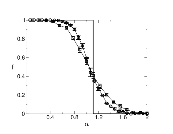
FIG. 1.: Fraction $f$ of $3\alpha N$ random input-output mappings implementable by a MLN with $3N$ inputs and $N$ hidden units as function of $\alpha$ for $N=3$ (squares) and $N=5$ (circles). The couplings between hidden units and output are fixed to $J_{i}=1$ for all $i$ and enumerations are performed over all combinations of symmetric Boolean functions $B_{i}$ between input and hidden layer. For every value of $\alpha$, 200 realizations of Gaussian inputs where averaged over. The solid line gives the analytical result describing the limit $N\to\infty$.

It is possible to generalize the above analysis to the case of discrete couplings with finite synaptic depth $l$ of the form $J_{i}=\pm 1/l,\pm 2/l,...,\pm 1$ by building on the analysis of the analogous case for the perceptron [7, 8]. In this case the additional order parameter $\bar{q}=\sum_{i}(J_{i}^{a})^{2}/N$, and its conjugate, $\hat{\bar{q}}$ have to be introduced. For $G_{E}$ we then again find (4) with now $Q=\sqrt{q/(\bar{q}-q)}$. Moreover $G_{C}=-\hat{\bar{q}}\bar{q}+\hat{q}q/2$ and, if all symmetrical Boolean functions are admissible,

$$G_{S} =\int\prod_{\boldsymbol{\xi}}Dz_{\boldsymbol{\xi}}$$ (8)

$$\ln\mathop{\rm Tr}_{J}\exp(-(\frac{\hat{q}}{2}-\hat{\bar{q}})J^{2})\prod_{\mathbf{\xi}}2\cosh(J\,\sqrt{\frac{\hat{q}}{2^{L-1}}}\;z_{\mathbf{\xi}}),$$ (9)

with $\mathop{\rm Tr}_{J}$ denoting the trace over the $2l$ possible values of the couplings $J_{i}$. Using these results we have numerically calculated the storage capacity $\alpha_{c}(l)$ for the simplest case $L=3$ as a function of the synaptic depth $l$. The results are shown in fig.2 together with a fit to the asymptotic behavior. The capacity increases from $\alpha_{c}\cong 1.11$ of the Ising case, $\l=1$, to roughly $1.7$ for large $l$. It is rather difficult to compare these analytical findings with numerical simulations since the effects of the finite synaptic depth do not show up at the small values of $N$ accessible to exact enumerations [9].

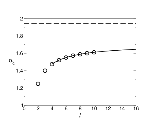
FIG. 2.: Storage capacity of a MLN with $N\to\infty$ hidden units and $3N$ inputs with couplings $J_{i}$ between hidden layer and output taking $2l$ discrete values. The inputs are mapped to the hidden layer by symmetric Boolean functions $B_{i}$. The solid line is the fit $\alpha_{c}\sim 1.70-0.91/l$ to the asymptotic behavior, the dashed line gives the replica symmetric result for continuous couplings $J_{i}$.

To complete the analysis of the storage properties we analyze the case of continuous couplings ${\mathbf{J}}$ between hidden and output layer. It is convenient to eliminate the additional order parameter $k$ necessary in this case to enforce the normalization ${\mathbf{J}}^{2}=N$ by introducing $\hat{Q}=\hat{q}/(k+\hat{q})$. Within replica symmetry the quenched entropy $s$ is then again of the form (3) with $G_{C}=0$, $G_{E}$ given by (4), and the extremum taken now over $Q$ and $\hat{Q}$. Moreover

$$G_{S}= \frac{1}{2}\ln(1-\frac{\hat{Q}}{1+Q^{2}})$$ (10)

$$+\int\prod_{\boldsymbol{\xi}}Dz_{\boldsymbol{\xi}}\ln\mathop{\rm Tr}_{B}\;\exp(\frac{\hat{Q}}{2^{L}}\;(\sum_{\boldsymbol{\xi}}z_{\boldsymbol{\xi}}B({\boldsymbol{\xi}}))^{2}).$$ (11)

The storage capacity $\alpha_{c}$ can be obtained from these expressions in the limits $Q\to\infty,\hat{Q}\to\infty$ corresponding to $q\to 1$. This limit indicates that different solutions of the storage problem may at most differ in a non-extensive number of components $J_{i}$ and Boolean functions $B_{i}$. We then find $G_{E}\sim-Q^{2}/4$ and, if all Boolean functions are admissible, $G_{S}\sim\hat{Q}(1/2+(2^{L-1}-1)/\pi)$ giving rise to

$$\alpha_{c}^{RS}=\frac{2+\frac{4}{\pi}(2^{L-1}-1)}{L}.$$ (12)

For $L=3$ this yields $\alpha_{c}^{RS}=2/3+4/\pi\cong 1.94$. If only linearly separable Boolean functions implementable by coupling vectors ${\mathbf{w}}_{i}$ are considered the asymptotic behavior of $G_{S}$ is more difficult to obtain. For the case $L=3$ we find $\alpha_{c}\cong 1.85$. Again the relative reduction of $\alpha_{c}$ when compared to the unrestricted case is roughly given by the ratio of the logarithms of the number of available Boolean functions per hidden unit.

It is possible to derive an upper bound for $\alpha_{c}$ as has been done for MLN with a finite number of hidden units [10] by using some exact results for the perceptron [11]. For $L=3$ we find $\alpha_{c}(L=3)\leq 2.394$ and the replica symmetric result is therefore within the bound. For large $L$ the bound is given by $\alpha_{c}(L\to\infty)\lesssim 2^{L-1}/L+\ln 2$ and shows the same scaling with $L$ as (12). Nevertheless the replica symmetric result (12) is very likely to overestimate the storage capacity as can be seen from fig.2 in which the result for $\alpha_{c}$ for $L=3$ is included as horizontal dashed line. Unlike the case of the perceptron [7] the values for $\alpha_{c}$ for finite synaptic depth seem not to approach the value for continuous couplings when $l\to\infty$. It would hence be very interesting to investigate the implications of replica symmetry breaking, both on the case of continuous couplings and of couplings with finite synaptic depth [12].

Let us finally elucidate the generalization problem, i.e. the ability of the network to infer a rule from examples. To this end we consider as usual two networks of the same type with the couplings and Boolean function of one of them (the “teacher”) fixed at random. The other network (the “student”) receives a set of randomly chosen inputs ${\boldsymbol{\xi}}^{\mu}_{i},\mu=1,...,\alpha LN$ together with the corresponding outputs $\sigma^{\mu}_{T}$ generated by the teacher. The task for the student is to imitate the teacher as well as possible. The success in doing so is quantified by the generalization error $\varepsilon$ defined as the probability that a newly chosen random input is classified differently by teacher and student.

As is well known the statistical mechanics analysis of the generalization problem builds again on the expression (1) for the quenched entropy with the number of replicas now tending to 1 rather than to 0 [13, 2]. A nice feature of this limit is that replica symmetry is known to be stable. The order parameter $q$ defined in (2) now gives the typical overlap between teacher and student and determines the generalization error $\varepsilon$ in a simple way. In the present situation we have the standard relation $\varepsilon=(\arccos q)/\pi$. Moreover (4) is replaced by

$$G_{E}(q)=2\int Dt\;H(Q\;t)\;\ln H(Q\;t).$$ (13)

The case using Ising couplings $J_{i}=\pm 1$ and all symmetric Boolean functions can again be mapped exactly on the Ising perceptron. Correspondingly there is a discontinuous transition to perfect learning, $\varepsilon=0$ for $\alpha>\alpha_{d}$ [14] with $\alpha_{d}=1.24\;2^{L-1}/L$. This transition occurs when all Boolean functions of the student “lock” onto the corresponding input-hidden mappings of the teacher and is also expected to occur in the case where only a restricted set of Booleans can be implemented.

For continuous couplings we find $G_{C}=Q^{2}\hat{Q}/((1+Q^{2})(1-\hat{Q}))$ and

$$G_{S}=\frac{1}{2}\ln(1-\hat{Q})+\sqrt{1-\hat{Q}}\int\prod_{\boldsymbol{\xi}}Dz_{\boldsymbol{\xi}}\;g(z_{\boldsymbol{\xi}})\,\ln g(z_{\boldsymbol{\xi}})$$ (14)

where

$$g(z_{\boldsymbol{\xi}})=\mathop{\rm Tr}_{B}\exp(\frac{\hat{Q}}{2^{L}}(\sum_{\boldsymbol{\xi}}\,z_{\boldsymbol{\xi}}B(\boldsymbol{\xi}))^{2}).$$ (15)

For small $\alpha$ this gives rise to $\varepsilon\sim 1/2-\alpha L/(\pi^{2}2^{L-1})$ which coincides with the result for the perceptron for L=1 as it should. With increasing $L$ the initial decay of the generalization error becomes slower reflecting the increasing complexity and storage abilities of the network. There is no retarded learning because of the non-zero correlation between the hidden units and the output [15]. For large $\alpha$ the generalization behaviour is dominated by the fine tuning of the student couplings between hidden layer and output to the respective couplings of the teacher resulting in the ubiquitous power law decay $\varepsilon\sim 0.625/(L\alpha)$.

In conclusion we have quantitatively characterized the storage and generalization abilities of a multilayer neural network with a number of hidden units scaling as the input dimension. If the mapping from the input to the hidden layer is realized by symmetric Boolean functions with $L$ inputs the capacity is found to be proportional to the logarithm of the number of these Boolean functions divided by $L$. The more conventional case in which the hidden units are the outputs of perceptrons with couplings ${\mathbf{w}}_{i}$ is more difficult to analyze. However, speculating that the above scaling holds true also in this case and observing that the logarithm of the number of Boolean functions which can be implemented by a perceptron with $L$ inputs is $O(L^{2})$ we arrive at the interesting result that the number of stored input-output relations per weight of the network is proportional to $L$. This implies that doubling the number of couplings in the network would increase the storage capacity by a factor of 2 making the proposed architecture superior to MLN with few ($K\ll N$) hidden units in which the storage capacity is known to increase at most logarithmically with the number of weights.

Acknowledgment: We have benefitted from discussions with Wolfgang Kinzel, Robert Urbanczik, Peter Reimann, and Stephan Mertens. We would like to thank the Max-Planck-Institut für Physik komplexer Systeme in Dresden where this work was finished for hospitality and the GIF for support.

REFERENCES

- [1] E. Gardner, J. Phys. A21, 257 (1988); E. Gardner and B. Derrida, J. Phys. A21, 271 (1988).
- [2] A. Engel and C. Van den Broeck Statistical Mechanics of Learning (Cambridge University Press, Cambrigde, 2001).
- [3] G. Cybenko, Math. Contr. Sign. Syst. 2, 303 (1989).
- [4] E. Barkai, D. Hansel and I. Kanter, Phys. Rev. Lett. 18, 2312 (1990); E. Barkai, D. Hansel, and H. Sompolinsky, Phys. Rev. A45, 4146 (1992); A. Engel, H. M. Köhler, F. Tschepke, H. Vollmayr, and A. Zippelius, Phys. Rev. A45, 5790 (1992); H. Schwarze and J. Hertz, Europhys. Lett. 20, 375 (1992); R. Monasson and R. Zecchina, Phys. Rev. Lett. 75, 2432 (1995); R. Urbanczik, Europhys. Lett. 35, 553 (1996); one of the rare exceptions is [5].
- [5] A. Bethge, R. Kühn, and H. Horner, J. Phys. A27, 1929 (1994).
- [6] W. Krauth and M. Mezard, J. Phys. (Paris) 50, 3057, 1989.
- [7] H. Gutfreund and Y. Stein, J. Phys. A23, 2613, 1990.
- [8] I. Kanter, Europhys. Lett. 17, 181, 1992.
- [9] A. Priel, M. Blatt, T. Grossman, E. Domany and I. Kanter Phys. Rev. E50, 577 (1994).
- [10] G. J. Mitchison and R. M. Durbin, Biol. Cybern. 60, 345 (1989).
- [11] T. M. Cover, IEEE Trans. Electron. Comput. EC-14, 326 (1965).
- [12] R. Urbanczik, Europhys. Lett. 26, 233 (1994)
- [13] M. Opper and D. Haussler, Phys. Rev. Lett. 66 , 2677 (1991).
- [14] G. Györgyi, Phys. Rev. A41, 7097 (1990).
- [15] M. Biehl and A. Mietzner, J. Phys. A 27, 1885 (1994); B. Schottky, J. Phys. A28, 4515 (1995); C. Van den Broeck and P. Reimann, Phys. Rev. Lett. 76, 2188 (1996).