Dissipation in Dynamics of a Moving Contact Line

Abstract

The dynamics of the deformations of a moving contact line is studied assuming two different dissipation mechanisms. It is shown that the characteristic relaxation time for a deformation of wavelength $2\pi/|k|$ of a contact line moving with velocity $v$ is given as $\tau^{-1}(k)=c(v)|k|$. The velocity dependence of $c(v)$ is shown to drastically depend on the dissipation mechanism: we find $c(v)=c(v=0)-2v$ for the case when the dynamics is governed by microscopic jumps of single molecules at the tip (Blake mechanism), and $c(v)\simeq c(v=0)-4v$ when viscous hydrodynamic losses inside the moving liquid wedge dominate (de Gennes mechanism). We thus suggest that the debated dominant dissipation mechanism can be experimentally determined using relaxation measurements similar to the Ondarcuhu-Veyssie experiment [T. Ondarcuhu and M. Veyssie, Nature 352, 418 (1991)].

I Introduction

Spreading of a liquid on a solid surface usually involves a rather complex dynamical behavior, which is determined by a subtle competition between the mutual interfacial energetics of the coexisting phases (the solid, the liquid, and the corresponding equilibrium vapor), dissipation processes and geometrical or chemical irregularities of the solid surface [1]. Interestingly, this dynamics can be effectively studied in terms of the dynamics of the contact line, which is the common borderline between the three phases, by correctly taking into account the physical processes in the vicinity of it.

One of the key issues about this dynamics which has remained a subject of controversy is dissipation. There are two rival theories in the literature, each depicting a different physical picture for the dominant dissipation mechanism in the dynamics of partial wetting [2]. The first approach, which is based on the idea of Yarnold and Mason [3] and was later developed into a quantitative theory by Blake and coworkers [4], emphasizes the role of microscopic jumps of single molecules (from the liquid into the vapor) in the immediate vicinity of the contact line. The other approach, which was developed by de Gennes and coworkers [1, 5], asserts that for small values of contact angle the dissipation is dominated by viscous hydrodynamic losses inside the moving liquid wedge.

For a partially wetting fluid on sufficiently smooth substrates, a contact line at equilibrium has a well defined contact angle $\theta_{e}$ that is determined by the solid-vapor $\gamma_{SV}$ and the solid-liquid $\gamma_{SL}$ interfacial energies, and the liquid surface tension $\gamma$ through Young’s relation: $\gamma_{SV}-\gamma_{SL}=\gamma\cos\theta_{e}$. For a moving contact line, however, the value of the so-called dynamic contact angle $\theta_{d}$ changes as a function of velocity: $\theta_{d}>\theta_{e}$ for an advancing contact line and $\theta_{d}<\theta_{e}$ for a receding one. Since the discrepancy between the two dissipation mechanisms appears for small contact angles [2], one can expect that receding contact lines are in fact very good candidates for experimental determination of the dominant mechanism in this regime.

A classic such example corresponds to wetting of a plate that is vertically withdrawn from a liquid at a constant velocity $-v$, which was first studied by Landau and Levich for complete wetting [6]. In the case of partial wetting that was studied by de Gennes [5, 7], a steady state is achieved in which the liquid will partially wet the plate with a nonvanishing dynamic contact angle $\theta_{d}(v)$ only for pull-out velocities less than a certain critical value $v_{c}$. The dynamic contact angle decreases with increasing $v$, until at the critical velocity the system undergoes a dynamical phase transition in which a macroscopic Landau–Levich liquid film, formally corresponding to a vanishing $\theta_{d}$, will remain on the plate.

Since the onset of leaving a film occurs at small values of contact angle, one can imagine that the two different dissipation mechanisms would lead to conflicting predictions about the transition. In particular, in Blake’s picture the “order parameter” for the transition $\theta_{d}$ would vanish continuously as $v$ approaches $v_{c}$, which makes it look like a second order phase transition. On the contrary, de Gennes predicts a jump in the order parameter from $\theta_{e}/\sqrt{3}$ to zero at the transition, which is the signature of a first order phase transition [2, 5]. This drastic difference in the predictions of the two theories can provide a reliable venue for testing them. However, such experiments have so far proven to be inconclusive due to the usual difficulties of tuning into a critical point in the presence of disorder [8].

Another notable feature of contact lines is their anomalous elasticity as noticed by Joanny and de Gennes [9]. For length scales below the capillary length (which is of the order of 3 mm for water at room temperature), a contact line deformation of wavevector $k$, denoted as $h(k)$ in Fourier space, will distort the surface of the liquid over a distance $|k|^{-1}$. Assuming that the surface deforms instantaneously in response to the contact line, the elastic energy cost for the deformation can be calculated from the surface tension energy stored in the distorted area, and is thus proportional to $|k|$, namely [9]

$$E_{\rm cl}={\gamma\theta_{e}^{2}\over 2}\int{dk\over 2\pi}|k||h(k)|^{2}.$$ (1)

The anomalous elasticity leads to interesting equilibrium dynamics, corresponding to when the contact line is perturbed from its static position, as studied by de Gennes [10]. Balancing ${dE_{\rm cl}\over dt}$ and the dissipation, which he assumes for small contact angles is dominated by the hydrodynamic dissipation in the liquid nearby the contact line, he finds that each deformation mode relaxes to equilibrium with a characteristic inverse decay time $\tau^{-1}(k)=c_{0}|k|$, in which $c_{0}={\gamma\theta_{e}^{3}/(3\eta\ell)}$ where $\eta$ is the viscosity of the liquid and $\ell$ is a logarithmic factor of order unity [10]. The relaxation is thus characterized by a linear dispersion relation, which implies that a deformation in the contact line will decay and propagate at a constant velocity $c_{0}$, as opposed to systems with normal line tension elasticity, where the decay and the propagation are governed by diffusion. This behavior has been observed, and the linear dispersion relation has been precisely tested, in a very interesting experiment by Ondarcuhu and Veyssie [11].

Here we study the dynamics of the deformations of a moving contact line for the two different dissipation mechanisms. In particular, we focus on the sizeable regime where the contact line is moving, i.e. it is away from the depinning transition [12], but still not too close to the onset of leaving a film. We show that in this regime the characteristic relaxation time for a $k$-mode deformation is given as $\tau^{-1}(k)=c(v)|k|$. The velocity dependence of $c(v)$ is shown to drastically depend on the dissipation mechanism: we find $c(v)=c(v=0)-2v$ in Blake’s scheme, whereas in de Gennes’ picture $c(v)$ might be rather well represented by $c(v)\simeq c(v=0)-4v$. We thus suggest that monitoring the deformation dynamics in this regime, along the lines of Ondarcuhu-Veyssie experiment [11], can provide a more practical probe for experimental determination of the debated dominant dissipation mechanism.

The rest of the paper is organized as follows. In Sec. II, we discuss the two different dissipation mechanisms and derive expressions for the corresponding energy dissipation rates. These expressions are then used in Sec. III to derive the force balance, and thus the governing dynamical equation. The velocity dependence of the dynamic contact angle and a characteristic velocity are studied in Secs. IV and V correspondingly. While Sec. VI discusses the effects of surface disorder, we conclude with some discussions in Sec. VII.

II Dissipation

Let us assume that the contact line is directed on average along the $x$ axis, and is moving in the $y$ direction with an average velocity $v$, which we assume to be positive corresponding to receding contact lines, as in Fig. 1. We can describe the position of the contact line along the $y$ axis for any given $x$ and $t$ with the function $y(x,t)=vt+h(x,t)$. We further assume that the deformation $h(x,t)$ is only a relatively small perturbation. We can now try to evaluate the overall dissipation for the deforming contact line within the two different scenarios.

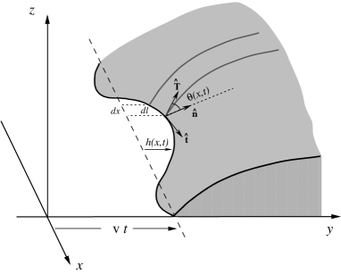
FIG. 1.: The schematics of the system.

A Blake approach

The physical process that is involved in causing dissipation in Blake’s picture, i.e. molecular jumps near the contact line, is local in nature [4]. Therefore, in any small neighborhood the amount of dissipation is completely determined by the local value of the contact line velocity, while all the molecular details of the dissipation is encoded in an effective friction coefficient $\mu^{-1}$. The overall dissipation can then be written as

$$P_{l}={1\over 2\mu}\int dx\left[v+\partial_{t}h(x,t)\right]^{2}.$$ (2)

In the limit of relatively small contact angles, which is relevant for our receding contact lines, the inverse friction coefficient (or mobility) can be calculated as [2]

$$\mu=\frac{k\lambda^{3}}{k_{B}T}\exp\left(-{W\over k_{B}T}\right),$$ (3)

in which $W$ is an activation energy for molecular hopping, $\lambda$ is the distance between hopping sites, $k$ is a characteristic “attempt” rate, and $k_{B}T$ is the thermal energy.

B de Gennes approach

We now focus on the contribution of dissipation that comes from the viscous losses in the hydrodynamic flows inside the liquid wedge [1, 5]. For a slightly deformed contact line, we assume that the dissipation can be approximated by the sum of contributions from wedge-shaped slices with local contact angles $\theta(x,t)$, as shown in Fig. 1. This is a reasonable approximation because most of the dissipation is taking place in the singular flows near the tip of the wedge [1, 5, 10]. Using the result for the dissipation in a perfect wedge, which is based on the lubrication approximation [1, 13], we can calculate the total dissipation as [10]

$$P_{h}={\eta\over 2}\int dx\left({3\ell\over\theta(x,t)}\right)\left[v+\partial_{t}h(x,t)\right]^{2},$$ (4)

in which $\ell=\ln(d_{max}/d_{min})$ with $d_{max}$ given by the size of the liquid drop and $d_{min}$ being a microscopic length scale. The inverse dependence on $\theta$ suggests that for sufficiently small contact angles the hydrodynamic loss is to be dominant [2].

III Force balance and dynamical equation

To find the governing dynamical equation in the long time limit, we should balance the total friction force obtained as $\delta(P_{l}+P_{h})/\delta\partial_{t}h(x,t)$ with the interfacial force $\gamma\cos\theta(x,t)-(\gamma_{SV}-\gamma_{SL})=\gamma[\cos\theta(x,t)-\cos\theta_{e}]$ at each point along the contact line. Note that in this section we are taking both dissipation mechanisms into account. In the limit of small contact angles, we find

$$\left[{1\over\mu}+{3\eta\ell\over\theta(x,t)}\right]\times\left[v+\partial_{t}h(x,t)\right]={\gamma\over 2}\left[\theta_{e}^{2}-\theta(x,t)^{2}\right].$$ (5)

To proceed from here, we need to relate the contact angle $\theta(x,t)$ to the contact line profile $h(x,t)$, which can be done through solving for the surface profile of the liquid drop. One can show that the surface profile $z(x,y)$ near the contact line can be found as a solution of the Laplace equation $(\partial^{2}_{x}+\partial^{2}_{y})z(x,y)=0$, so as to minimize the surface area. The solution that satisfies the boundary condition $z(x,h(x,t))=0$ reads [9]

$$z(x,y)=\theta_{d}\left[y-\int{dk\over 2\pi}h(k,t)e^{ikx-|k|y}\right],$$ (6)

from which we obtain

$$\theta(x,t)\equiv\left.{\partial z(x,y)\over\partial y}\right|_{y=h(x,t)}=\theta_{d}\left[1+\int{dk\over 2\pi}|k|h(k,t)e^{ikx}\right],$$ (7)

to the leading order [9].

To the zeroth order, Eq.(5) gives the relation between the average dynamic contact angle and the velocity as

$$v=\left(\gamma\over 6\eta\ell\right){\theta_{d}(\theta_{e}^{2}-\theta_{d}^{2})\over 1+{\theta_{d}/(3\eta\mu\ell)}}.$$ (8)

This relation will be used below to study the onset of the transition of the moving liquid drop to a Landau-Levich film.

The dynamical equation (Eq.(5)), which governs the dynamics of the deformation field, can now be written in the linear approximation as

$$\partial_{t}h(k,t)=-c(v)|k|h(k,t),$$ (9)

in Fourier space, where

$$c(v)={\mu\gamma\theta_{d}^{3}(v)-3\eta\mu\ell v\over 3\eta\mu\ell+\theta_{d}(v)},$$ (10)

with $\theta_{d}(v)$ to be found by inverting Eq.(8). The corresponding form of the dynamical equation in real space can be found by Fourier transformation as

$$\partial_{t}h(x,t)=-c(v)\int{dx^{\prime}\over\pi}{h(x^{\prime},t)\over(x-x^{\prime})^{2}},$$ (11)

which reflects the non-locality of the dynamics.

Relaxation of the contact line’s shape while it is moving thus takes place with the same dispersion relation $\tau^{-1}(k)\sim|k|$ as a contact line at rest, although the corresponding characteristic velocity $c(v)$ shows a strong dependence on the contact line velocity $v$.

IV Contact angle–velocity relation

There can be two types of experiments on a moving contact line depending on how we prepare it. We can fix a value for the contact angle that is different from $\theta_{e}$, and let it move with an adjusted velocity when it reaches a steady state. This can be achieved, for example, by adding or removing some volume of liquid through a syringe that is inserted in a liquid drop at equilibrium. On the contrary, we can fix the velocity and let the contact angle adjust itself in a steady state. This will be the case, for example, when a plate is withdrawn vertically from a liquid at a constant velocity.

Depending on which “ensemble” we are using, we will have a fixed value for $v$ or $\theta_{d}$, and we should then use Eq.(8) (that relates the velocity and the dynamic contact angle) to determine the conjugate parameter. The term “ensemble” is in fact quite appropriate to use here because the two (mechanically) conjugate quantities are, in fact, velocity and force–which is determined solely by the contact angle. What we have is then either a “constant velocity” or a “constant force” experiment. It is interesting to note that in non-equilibrium systems, in general, different ensembles may not necessarily lead to the same result [14].

In this work, we are mostly interested in constant velocity experiments, and thus we will treat $v$ as a fixed and given parameter below unless otherwise specified. We will examine Eq.(8) in the limiting cases corresponding to the two different dissipation mechanisms and compare their predictions.

A Blake approach

The behavior in this regime can be extracted from Eq.(8) by taking the limit $\mu\eta\ll\theta_{d}$. Inverting the resulting equation yields

$$\left.\theta_{d}(v)\over\theta_{e}\right|_{l}=\sqrt{1-{2v\over c_{l0}}},$$ (12)

in which $c_{l0}=\mu\gamma\theta_{e}^{2}$. Note that this holds only for $v<c_{l0}/2$, while $\theta_{d}=0$ identically for $v>c_{l0}/2$. This function is plotted in Fig. 2.

As can be readily seen from Fig. 2, increasing $v$ would lead to decreasing values of $\theta_{d}$ until at a critical velocity $v_{lc}=c_{l0}/2$ it finally vanishes continuously. A vanishing contact angle presumably corresponds to formation of a liquid film; a so-called Landau-Levich film. The value of the dynamic contact angle $\theta_{d}$ serves as the order parameter for this dynamical phase transition, while $v$ is the tuning parameter. The continuous vanishing of the order parameter makes the phase transition classified as second order. As in the general theory of critical phenomena, a mean-field exponent $\beta=1/2$ is characterizing the vanishing of the order parameter in terms of the tuning parameter.

FIG. 2.: The reduced order parameter $T_{l}=(\theta_{d}/\theta_{e})_{l}$ as a function of the dimensionless velocity $V_{l}=v/c_{l0}$ for Blake mechanism (Eq.(12)). The dynamical phase transition at $V_{lc}=1/2$ is predicted to be of second order in this picture.

B de Gennes approach

In the opposite limit of $\mu\eta\gg\theta_{d}$, only the hydrodynamic contribution survives, and Eq.(8) leads to

$$\left.\theta_{d}(v)\over\theta_{e}\right|_{h} = {1\over\sqrt{3}}\left[\left(-\nu-i\sqrt{1-\nu^{2}}\right)^{1/3}\right.$$ (14)

$$\left.+\left(-\nu+i\sqrt{1-\nu^{2}}\right)^{1/3}\right],$$

in which $\nu=3\sqrt{3}v/c_{h0}$ and $c_{h0}=\gamma\theta_{e}^{3}/(3\eta\ell)$.

FIG. 3.: The reduced order parameter $T_{h}=(\theta_{d}/\theta_{e})_{h}$ as a function of the dimensionless velocity $V_{h}=v/c_{h0}$ for de Gennes mechanism (Eq.(14)). The dynamical phase transition at $V_{hc}=1/(3\sqrt{3})\simeq 0.192$ is predicted to be of first order in this picture.

The above formula, which holds only for $v<c_{h0}/(3\sqrt{3})$ has two branches and only the one that recovers $\theta_{d}(0)=\theta_{e}$ is acceptable as plotted in Fig.3. While at $v=c_{h0}/(3\sqrt{3})$ we find $\theta_{d}=\theta_{e}/\sqrt{3}$, we expect to have $\theta_{d}=0$ for higher velocities $v>c_{h0}/(3\sqrt{3})$. Therefore, the order parameter $\theta_{d}$ experiences a finite jump at the transition velocity $v_{hc}=c_{h0}/(3\sqrt{3})$, that is the hallmark of a first order phase transition.

V Characteristic velocity

Using Eq.(10), and $\theta_{d}(v)$ that we have found in the previous section for the two different cases, we can extract the $v$-dependence of the characteristic velocity.

A Blake approach

We can simplify Eq.(10) by taking the limit $\mu\eta\ll\theta_{d}$, as

$$c_{l}(\theta)=c_{l0}{\theta_{d}^{2}\over\theta_{e}^{2}}.$$ (15)

Inserting the form of $\theta_{d}(v)$ from Eq.(12) yields

$$c_{l}(v)=c_{l0}-2v.$$ (16)

Note that in this approach $c(v)$ is strictly linear in $v$ all the way, and it vanishes at the transition point, as plotted in Fig. 4.

FIG. 4.: The reduced characteristic velocity $C_{l}=c_{l}/c_{l0}$ as a function of the dimensionless velocity $V_{l}=v/c_{l0}$ for Blake mechanism (Eq.(16)). The slope of the curve is $-2$ all the way to the transition point where the characteristic velocity vanishes.

B de Gennes approach

In the opposite limit of $\mu\eta\gg\theta_{d}$, Eq.(10) will be simplified as

$$c_{h}(\theta)={c_{h0}\over 2}\left(3{\theta_{d}^{3}\over\theta_{e}^{3}}-{\theta_{d}\over\theta_{e}}\right).$$ (17)

Putting in $\theta_{d}(v)$ from Eq.(14) leads to

$$c_{h}(v) = {c_{h0}\over\sqrt{3}}\left[\left(-\nu-i\sqrt{1-\nu^{2}}\right)^{1/3}\right.$$ (19)

$$\left.+\left(-\nu+i\sqrt{1-\nu^{2}}\right)^{1/3}-\nu\right].$$

One can again check from this equation that $c(v)$ vanishes at the transition. The above equation is plotted in Fig. 5.

FIG. 5.: The reduced characteristic velocity $C_{h}=c_{h}/c_{h0}$ as a function of the dimensionless velocity $V_{h}=v/c_{h0}$ for de Gennes mechanism (Eq.(19)). The slope of the curve is nearly $-4$ until a square-root singularity sets in near the transition point where the characteristic velocity vanishes.

The characteristic velocity can be well approximated by the linear expression

$$c_{h}(v)\simeq c_{h0}-4v,$$ (20)

for a wide range of $v$, except very near $c_{h0}/(3\sqrt{3})$ where it experiences a square-root singular behavior as

$$c_{h}(v) \simeq c_{h0}\left[\sqrt{2}\left({1\over 3\sqrt{3}}-{v\over c_{h0}}\right)^{1/2}+3\left({1\over 3\sqrt{3}}-{v\over c_{h0}}\right)\right.$$ (22)

$$\left.+O\left(\left({1\over 3\sqrt{3}}-{v\over c_{h0}}\right)^{3/2}\right)\right].$$

It is interesting to note that although both approaches predict a sizeable linear regime for $c(v)$, as manifest in Eqs.(16) and (20), the corresponding slopes are predicted differently.

VI Surface Disorder

In most practical cases, the dynamics of a contact line is affected by the defects and heterogeneities in the substrate, in addition to dissipation and elasticity that we have considered so far. If the interfacial energies $\gamma_{SV}$ and $\gamma_{SL}$ are space dependent with the corresponding averages being ${\bar{\gamma}_{SV}}$ and ${\bar{\gamma}_{SL}}$, a displacement $\delta y(x,t)$ of the contact line is going to lead to a change in energy as

$$\delta E_{d}=\int dxg(x,vt+h(x,t))\delta y(x,t),$$ (23)

where

$$g(x,y)=\gamma_{SV}(x,y)-\gamma_{SL}(x,y)-({\bar{\gamma}_{SV}}-{\bar{\gamma}_{SL}}).$$ (24)

Incorporating this contribution in the force balance leads to an extra force term $g(x,vt)$ on the right hand side of Eq.(5), and thus a noise term on the right hand side of Eq.(11) of the form

$$\eta(x,t)=\left({\mu\theta_{d}\over\theta_{d}+3\eta\mu\ell}\right)g(x,vt),$$ (25)

to the leading order. Note that this is a good approximation provided we are well away from the depinning transition, and the contact line is moving fast enough [1, 9, 12, 16].

Assuming that the surface disorder has short range correlations with a Gaussian distribution described by

$$\langle g(x,y)\rangle = 0,$$ (26)

$$\langle g(x,y)g(x^{\prime},y^{\prime})\rangle = g^{2}a^{2}\delta(x-x^{\prime})\delta(y-y^{\prime}),$$ (27)

we can deduce the distribution of the noise as

$$\langle\eta(x,t)\rangle = 0,$$ (28)

$$\langle\eta(x,t)\eta(x^{\prime},t^{\prime})\rangle = 2D(v)\delta(x-x^{\prime})\delta(t-t^{\prime}),$$ (29)

where

$$D(v)={g^{2}a^{2}\over 2v}\left({\mu\theta_{d}(v)\over\theta_{d}(v)+3\eta\mu\ell}\right)^{2}.$$ (30)

In the presence of the noise, the contact line undergoes dynamical fluctuations. These fluctuations can best be characterized by the width of the contact line, which is defined as

$$W^{2}(L,t)\equiv{1\over L}\int dx\langle h(x,t)^{2}\rangle.$$ (31)

Using Eq.(9) with the noise term, we can calculate the width of the contact line as

$$W^{2}(L,t) = {D(v)\over\pi c(v)}\times\int_{\pi/L}^{\pi/a}{dk\over k}\left[1-e^{-2c(v)|k|t}\right]$$ (32)

$$= {D(v)\over\pi c(v)}\times\left\{\begin{array}[]{ll}\ln\left[c(v)t/a\right],&\;{a\over c(v)}\ll t\ll{L\over c(v)},\\ \ln\left(L/a\right),&\;t\gg{L\over c(v)},\end{array}\right.$$ (35)

Similarly, we can study the fluctuations in the order parameter field $\delta\theta(x,t)=\theta(x,t)-\theta_{d}$. Using Eqs.(7) and (9), we find

$$\langle\delta\theta(x,t)^{2}\rangle = {D(v)\theta_{d}^{2}(v)\over\pi c(v)}\times\int_{\pi/L}^{\pi/a}dk\;k\left[1-e^{-2c(v)|k|t}\right]$$ (36)

$$= {\pi D(v)\theta_{d}^{2}(v)\over 2c(v)a^{2}}\left(1-{a^{2}\over 2\pi^{2}c^{2}(v)t^{2}}\right),$$ (37)

for $t\gg a/c(v)$.

The magnitude of the fluctuations of the contact line width

$$\Delta(v)={D(v)\over\pi c(v)},$$ (38)

and, correspondingly, that of the order parameter

$$\sigma(v)={\pi D(v)\theta_{d}^{2}(v)\over 2c(v)a^{2}},$$ (39)

are thus both velocity dependent. Again, we expect this dependence to be different for the two cases.

A Blake approach

In this case we have $\mu\eta\ll\theta_{d}$, which together with Eqs.(12), (16), (30), (38), and (39) yield

$$\Delta_{l}(v)=\left({\mu^{2}g^{2}a^{2}\over 2\pi c_{l0}^{2}}\right)\times{1\over(v/c_{l0})(1-2v/c_{l0})},$$ (40)

and

$$\sigma_{l}(v)=\left({\pi\mu^{2}g^{2}\theta_{e}^{2}\over 4c_{l0}^{2}}\right)\times{1\over(v/c_{l0})}.$$ (41)

The above equations are plotted in Figs. 6 and 7. Fig. 6 shows that the width of the contact line is a symmetric function of velocity in this picture, while Fig. 7 denotes that the order parameter fluctuations decrease monotonically with velocity. Note also that these fluctuations remain finite at the transition point, which is not typical of second order phase transitions.

FIG. 6.: The reduced width $A_{l}=\Delta_{l}/\left({\mu^{2}g^{2}a^{2}\over 2\pi c_{l0}^{2}}\right)$ as a function of the dimensionless velocity $V_{l}=v/c_{l0}$ for Blake mechanism (Eq.(40)). It is symmetric with respect to $V_{l}=1/4$.

FIG. 7.: The reduced order parameter fluctuations $B_{l}=\sigma_{l}/\left({\pi\mu^{2}g^{2}\theta_{e}^{2}\over 4c_{l0}^{2}}\right)$ as a function of the dimensionless velocity $V_{l}=v/c_{l0}$ for Blake mechanism (Eq.(41)). It is a monotonically decreasing function of velocity. Note the unusual feature that the order parameter fluctuations remain finite at the transition point, unlike traditional second order phase transitions.

B de Gennes approach

Taking the opposite limit $\mu\eta\gg\theta_{d}$ in Eq.(30), together with Eqs.(14), (19), (38), and (39), we obtain

$$\Delta_{h}(v)=\left({g^{2}a^{2}\theta_{e}^{2}\over 6\pi\eta^{2}\ell^{2}c_{h0}^{2}}\right)\times\left\{\frac{\left[\left(-\nu-i\sqrt{1-\nu^{2}}\right)^{1/3}+\left(-\nu+i\sqrt{1-\nu^{2}}\right)^{1/3}\right]^{2}}{\nu\left[\left(-\nu-i\sqrt{1-\nu^{2}}\right)^{1/3}+\left(-\nu+i\sqrt{1-\nu^{2}}\right)^{1/3}-\nu\right]}\right\},$$ (42)

and

$$\sigma_{h}(v)=\left({\pi g^{2}\theta_{e}^{4}\over 36\eta^{2}\ell^{2}c_{h0}^{2}}\right)\times\left\{\frac{\left[\left(-\nu-i\sqrt{1-\nu^{2}}\right)^{1/3}+\left(-\nu+i\sqrt{1-\nu^{2}}\right)^{1/3}\right]^{4}}{\nu\left[\left(-\nu-i\sqrt{1-\nu^{2}}\right)^{1/3}+\left(-\nu+i\sqrt{1-\nu^{2}}\right)^{1/3}-\nu\right]}\right\}.$$ (43)

The above equations are plotted in Figs. 8 and 9. Fig. 8 shows that the width of the contact line is not a symmetric function of velocity in this case. Moreover, the order parameter fluctuations do not decrease monotonically with velocity as shown in Fig. 9. Unlike in the previous case, these fluctuations diverge at the transition point, which is again not typical of first order phase transitions.

FIG. 8.: The reduced width $A_{h}=\Delta_{h}/\left({g^{2}a^{2}\theta_{e}^{2}\over 18\pi\eta^{2}\ell^{2}c_{h0}^{2}}\right)$ as a function of the dimensionless velocity $V_{h}=v/c_{h0}$ for de Gennes mechanism (Eq.(42)). Note the asymmetry of the plot in this case.

FIG. 9.: The reduced order parameter fluctuations $B_{h}=\sigma_{h}/\left({\pi g^{2}\theta_{e}^{4}\over 36\eta^{2}\ell^{2}c_{h0}^{2}}\right)$ as a function of the dimensionless velocity $V_{h}=v/c_{h0}$ for de Gennes mechanism (Eq.(43)). In this case, it is not a monotonically decreasing function of velocity. Note the unusual feature that the order parameter fluctuations diverge at the transition point, unlike traditional first order phase transitions.

VII Discussion

Because of their anomalous elasticity, contact lines relax to their equilibrium from an initially distorted configuration with a characteristic inverse decay time $\tau^{-1}(k)=c(v)|k|$ for each $k$-mode. The $v$-dependence of the characteristic velocity $c(v)$ is shown to crucially depend on the dissipation mechanism, and it can thus be used as an experimental probe for the dominant dissipation mechanism.

A typical experiment for such investigations is direct monitoring of the contact line shape during the relaxation process. If the initial distortion of the contact line can be made periodic in a controlled way, like in the experiment of Ondarcuhu and Veyssie [11], one can directly map out $c(v)$ and hence determine the dissipation mechanism from its $v$-dependence.

Another possibility is to have relaxation from random initial distortions, which will be the case when we pull out a naturally rough plate from the liquid. Monitoring the dynamics of the contact line in this case will provide statistical information about the relaxation process, from which one can hope to deduce the relevant features discussed in Sec. VI.

We finally note that this linear theory is not sufficient for a complete understanding of the Landau-Levich phase transition, and it breaks down upon approaching the transition point. This breakdown is particularly manifest in the divergence that we encountered in the width of the contact line at the transition point. To be able to have a complete description, one should keep the relevant nonlinear terms that can be calculated by extending the method of this paper, and resort to perturbative renormalization group approaches for the resulting nonlinear stochastic equation. We have performed these studies, and the corresponding results will appear elsewhere [15].

In conclusion, we have studied the relaxation dynamics of the contact lines, and suggested that monitoring this dynamics can provide an experimental probe for the debated dominant dissipation mechanism.

REFERENCES

- [1] P.G. de Gennes, Rev. Mod. Phys. 57, 827 (1985).
- [2] F. Brochard-Wyart and P.G. de Gennes, Adv. Colloid Interface Sci. 39, 1 (1992).
- [3] G. Yarnold and B Manson, Proc. Phys. Soc. (London) B 62, 121 (1949); Proc. Phys. Soc. (London) B 62, 125 (1949).
- [4] T.D. Blake and J.M. Haynes, J. Colloid Interface Sci. 30, 421 (1969); T.D. Blake and K.J. Ruschak, Nature 282, 489 (1979); T. Blake in AIChE International Symposium on the mechanics of thin film coating (New Orleans, 1988).
- [5] P.G. de Gennes, Colloid & Polymer Sci. 264, 463 (1986); P.G. de Gennes, in Physics of Amphiphilic Layers eds. J. Meunier, D. Langevin, and N. Boccara (Springer, Berlin, 1987); F. Brochard-Wyart, J.M. di Meglio, and D. Quéré, C. R. Acad. Sci. (Paris) 304 II, 553 (1987).
- [6] L. Landau and B. Levich, Acta Physicochim. USSR 17, 42 (1942); B. Levich, Physicochemical Hydrodynamics (Prentice-Hall, London, 1962).
- [7] See also: O.V. Voinov, Fluid Dyn. Engl. Transl. 11, 714 (1976); R.G. Cox, J. Fluid Mech. 168, 169 (1986).
- [8] D. Quéré, private communication.
- [9] J.F. Joanny and P.G. de Gennes, J. Chem. Phys. 81, 552 (1984).
- [10] P.G. de Gennes, C. R. Acad. Sci. Paris II 302, 731 (1986).
- [11] T. Ondarcuhu and M. Veyssie, Nature 352, 418 (1991).
- [12] For a discussion of the depinning transition in contact lines see: E. Raphaël and P.G. de Gennes, J. Chem. Phys. 90, 7577 (1989); J.F. Joanny and M.O. Robbins, J. Chem. Phys. 92, 3206 (1990); D. Ertas and M. Kardar, Phys. Rev. E 49, R2532 (1994); E. Schäffer and P. Wong, Phys. Rev. Lett. 80, 3069 (1998); Phys. Rev. E 61, 5257 (2000); C. Guthmann, R. Gombrowicz, V. Repain, and E. Rolley, Phys. Rev. Lett. 80, 2865 (1998); A. Hazareesing and M. Mezard, Phys. Rev. E 60, 1269 (1999).
- [13] C. Huh and L. Scriven, J. Colloid Interface Sci. 35, 85 (1971).
- [14] For an example of different behavior of constant-force and constant-velocity ensembles in wetting systems see: E. Raphaël and P.G. de Gennes, J. Chem. Phys. 90, 7577 (1989); J.F. Joanny and M.O. Robbins, J. Chem. Phys. 92, 3206 (1990).
- [15] R. Golestanian and E. Raphaël, to appear in Europhys. Lett. (2001)(preprint cond-mat/0006496).
- [16] M.O. Robbins and J.F. Joanny, Europhys. Lett. 3, 729 (1987).