Tube Models for Rubber-Elastic Systems

Abstract

In the first part of the paper we show that the constraining potentials introduced to mimic entanglement effects in Edward’s tube model and Flory’s constrained junction model are diagonal in the generalized Rouse modes of the corresponding phantom network. As a consequence, both models can formally be solved exactly for arbitrary connectivity using the recently introduced constrained mode model. In the second part, we solve a double tube model for the confinement of long paths in polymer networks which is partially due to crosslinking and partially due to entanglements. Our model describes a non-trivial crossover between the Warner-Edwards and the Heinrich-Straube tube models. We present results for the macroscopic elastic properties as well as for the microscopic deformations including structure factors.

I Introduction

Polymer networks [1] are the basic structural element of systems as different as tire rubber and gels and have a wide range of technical and biological applications. From a macroscopic point of view, rubber-like materials have very distinct visco- and thermoelastic properties. [1, 2] They reversibly sustain elongations of up to 1000% with small strain elastic moduli which are four or five orders of magnitude smaller than for other solids. Maybe even more unusual are the thermoelastic properties discovered by Gough and Joule in the 19th century: when heated, a piece of rubber under a constant load contracts, and, conversely, heat is released during stretching. This implies that the stress induced by a deformation is mostly due to a decrease in entropy. The microscopic, statistical mechanical origin of this entropy change remained obscure until the discovery of polymeric molecules and their high degree of conformational flexibility in the 1930s. In a melt of identical chains polymers adopt random coil conformations [3] with mean-square end-to-end distances proportional to their length, $\left<\vec{r}^{2}\right>\sim N$. A simple statistical mechanical argument, which only takes the connectivity of the chains into account, then suggests that flexible polymers react to forces on their ends as linear, entropic springs. The spring constant, $k=\frac{3k_{B}T}{\left<\vec{r}^{2}\right>}$, is proportional to the temperature. Treating a piece of rubber as a random network of non-interacting entropic springs (the phantom model [4, 5, 6]) qualitatively explains the observed behavior, including — to a first approximation — the shape of the measured stress-strain curves.

In spite of more than sixty years of growing qualitative understanding, a rigorous statistical mechanical treatment of polymer networks remains a challenge to the present day. Similar to spin glasses, [7] the main difficulty is the presence of quenched disorder over which thermodynamic variables need to be averaged. In the case of polymer networks, [8, 9, 10] the vulcanization process leads to a simultaneous quench of two different kinds of disorder: (i) a random connectivity due to the introduction of chemical crosslinks and (ii) a random topology due to the formation of closed loops and the mutual impenetrability of the polymer backbones. Since for instantaneous crosslinking monomer-monomer contacts and entanglements become quenched with a probability proportional to their occurrence in the melt, ensemble averages of static expectation values for the chain structure etc. are not affected by the vulcanization as long as the system remains in its state of preparation.

For a given connectivity the phantom model Hamiltonian for non-interacting polymer chains formally takes a simple quadratic form, [4, 5, 6] so that one can at least formulate theories which take the random connectivity of the networks fully into account. [11, 12, 13] The situation is less clear for entanglements or topological constraints, since they do not enter the Hamiltonian as such, but divide phase space into accessible and inaccessible regions. In simple cases, entanglements can be characterized by topological invariants from mathematical knot theory. [8, 9] However, attempts to formulate topological theories of rubber elasticity (for references see [14]) encounter serious difficulties. Most theories therefore omit such a detailed description in favor of a mean-field ansatz where the different parts of the network are thought to move in a deformation-dependent elastic matrix which exerts restoring forces towards some rest positions. These restoring forces may be due to chemical crosslinks which localize random paths through the network in space [15] or to entanglements. The classical theories of rubber elasticity [1, 16, 17, 18, 19, 20] assume that entanglements act only on the crosslinks or junction points, while the tube models [2, 21, 22, 23, 24, 25, 26] stress the importance of the topological constraints acting along the contour of strands exceeding a minimum “entanglement length”, $N_{e}$. Originally devised for polymer networks, the tube concept is particularly successful in explaining the extremely long relaxation times in non-crosslinked polymer melts as the result of a one-dimensional, curvilinear diffusion called reptation [27] of linear chains of length $N\gg N_{e}$ within and finally out of their original tubes. Over the last decade computer simulations [14, 28, 29, 30] and experiments [31, 32, 33] have finally also collected mounting evidence for the importance and correctness of the tube concept in the description of polymer networks.

More than thirty years after its introduction and in spite of its intuitivity and its success in providing a unified view on entangled polymer networks and melts, [2, 23, 25, 26] there exists to date no complete solution of the Edwards tube model for polymer networks. Some of the open problems are apparent from a recent controversy on the interpretation of SANS data. [32, 33, 34, 35, 36, 37] Such data constitute an important experimental test of the tube concept, since they contain information on the degree and deformation dependence of the confinement of the microscopic chain motion and therefore allow for a more detailed test of theories of rubber elasticity than rheological data. [38, 39, 40]

On the theoretical side, the original approach of Warner and Edwards [15] used mathematically rather involved replica methods [26] to describe the localization of a long polymer chain in space due to crosslinking. The replica method allows for a very elegant, self-consistent introduction of constraining potentials, which confine individual polymer strands to random-walk like tubular regions in space while ensemble averages over all polymers remain identical to those of unconstrained chains. Later Heinrich and Straube [25, 32] recalculated these results for a solely entangled system where they argued that there are qualitative differences between confinement due to entanglements and confinement due to crosslinking. In particular, they argued that the strength of the confining potential should vary affinely with the macroscopic strain, resulting in fluctuations perpendicular to the tube axis which vary only like the square root of the macroscopic strain.

Replica calculations provide limited insight into physical mechanism and make approximations which are difficult to control. [12] It is therefore interesting to note that Flory was able to solve the, in many respects similar, constrained-junction model [17] without using such methods. Recent refinements of the constrained-junction model such as the constrained-chain model [41] and the diffused-constrained model [42] have more or less converged to the (Heinrich and Straube) tube model, even though the term is not mentioned explicitly. Another variant of this model was recently solved by Rubinstein and Panyukov. [43] In particular, the authors illustrated how non-trivial, sub-affine deformations of the polymer strands result from an affinely deforming confining potential.

While tube models are usually formulated and discussed in real space, two other recent papers have pointed independently to considerable simplifications of the calculations in mode space. Read and McLeish [35] were able to rederive the Warner-Edwards result in a particularly simple and transparent manner by showing that a harmonic tube potential is diagonal in the Rouse modes of a linear chain. Complementary, one of the present authors introduced a general constrained mode model (CMM), [44] where confinement is modeled by deformation dependent linear forces coupled to (approximate) eigenmodes of the phantom network instead of a tube-like potential in real space. This model can easily be solved exactly and is particularly suited for the analysis of simulation data, where its parameters, the degrees of confinement for all considered modes, are directly measurable. Simulations of defect-free model polymer networks under strain analyzed in the framework of the CMM [14] provide evidence that it is indeed possible to predict macroscopic restoring forces and microscopic deformations from constrained fluctuation theories. In particular, the results support the choice of Flory, [17] Heinrich and Straube, [25] and Rubinstein and Panyukov [43] for the deformation dependence of the confining potential. In spite of this success, the CMM in its original form suffers from two important deficits: (i) due to the multitude of independent parameters it is completely useless for a comparison to experiment and (ii) apart from recovering the tube model on a scaling level, Ref. [44] remained fairly vague on the exact relation between the approximations made by the Edwards tube model and the CMM respectively.

In the present paper we show that the two models are, in fact, equivalent. The proof, presented in section II B is a generalization of the result by Read and McLeish to arbitrary connectivity. It provides the link between the considerations of Eichinger,[11] Graessley, [45] Mark, [46] and others on the dynamics of (micro) phantom networks and the ideas of Edwards and Flory on the suppression of fluctuations due to entanglements. As a consequence, the CMM can be used to formally solve the Edwards tube model exactly, while in turn the independent parameters of the CMM are obtained as a function of a single parameter: the strength of the tube potential. Quite interestingly, it turns out that the entanglement contribution to the shear modulus depends on the connectivity of the network. In order to explore the consequences, we discuss in the second part the introduction of entanglement effects into the Warner-Edwards model, which represents the network as an ensemble of independent long paths comprising many strands. Besides recovering some results by Rubinstein and Panyukov for entanglement dominated systems, we also calculate the single chain structure factor for this controversial case. [32, 33, 34, 35, 36, 37] Finally we propose a “double tube” model to describe systems where the confinement of the fluctuations due to crosslinks and due to entanglements is of similar importance and where both effects are treated within the same formalism.

II Constrained fluctuations in networks of arbitrary connectivity

A The Phantom Model

The Hamiltonian of the phantom model [4, 5, 6] is given by ${\cal H}_{ph}=\frac{k}{2}\sum_{\left<i,j\right>}^{M}r_{ij}^{2}$, where ${\left<i,j\right>}$ denotes a pair of nodes $i,j\in{1,\ldots,M}$ which are connected by a polymer chain acting as an entropic spring of strength $k=\frac{3k_{B}T}{\left<\vec{r}^{2}\right>}$, and $\vec{r}_{ij}(t)=\vec{r}_{i}(t)-\vec{r}_{j}(t)$ the distance between them. In order to simplify the notation, we always assume that all elementary springs have the same strength $k$. The problem is most conveniently studied using periodic boundary conditions, which span the network over a fixed volume [10] and define the equilibrium position $\vec{R}_{i}=(X_{i},Y_{i},Z_{i})$. A conformation of a network of harmonic springs can be analyzed in terms of either the bead positions $\vec{r}_{i}(t)$ or the deviations $\vec{u}_{i}(t)$ of the nodes from their equilibrium positions $\vec{R}_{i}$. In this representation, the Hamiltonian separates into two independent contributions from the equilibrium extensions of the springs and the fluctuations. For the following considerations it is useful to write fluctuations as a quadratic form. [11] Finally, we note that the problem separates in Cartesian coordinates $\alpha=x,y,z$ due to the linearity of the springs. In the following we simplify the notation by writing the equations only for one spatial dimension:

$${\cal H}_{ph}=\frac{k}{2}\sum_{\left<i,j\right>}X_{ij\alpha}^{2}+\frac{1}{2}\,\underline{u}\,^{t}\underline{\underline{K}}\,\underline{u}\,.$$ (1)

Here ${\underline{u}\,}$ denotes a $M$-dimensional vector with $(\underline{u}\,)_{i}\equiv(\vec{u}_{i})_{x}$. $\underline{\underline{K}}\,$ is the connectivity or Kirchhoff matrix whose diagonal elements $(\underline{\underline{K}}\,)_{ii}=f_{i}k$ are given by the node’s functionality (e.g. a node which is part of a linear chain is connected to its two neighbors so that $f_{i}=2$ in contrast to a four-functional crosslink with $f_{i}=4$). The off-diagonal elements of the Kirchhoff matrix are given by $(\underline{\underline{K}}\,)_{ij}=-k$, if nodes $i$ and $j$ are connected and by $(\underline{\underline{K}}\,)_{ij}=0$ otherwise. Furthermore, we have assumed that all network strands have the same length.

The fluctuations can be written as a sum over independent modes $\underline{e}\,_{p}$ which are the eigenvectors of the Kirchhoff matrix: $\underline{\underline{K}}\,\underline{e}\,_{p}=k_{p}\underline{e}\,_{p}$ where the $\underline{e}\,_{p}$ can be chosen to be orthonormal $\underline{e}\,_{p}\cdot\underline{e}\,_{p\prime}=\delta_{pp\prime}$. The transformation to the eigenvector representation $\underline{\tilde{u}}\,=\underline{\underline{S}}\,\underline{u}\,$ and back to the node representation $\underline{u}\,=\underline{\underline{S}}\,^{-1}\underline{\tilde{u}}\,$ is mediated by a matrix $\underline{\underline{S}}\,$ whose column vectors correspond to the $\underline{e}\,_{p}$. By construction, $\underline{\underline{S}}\,$ is orthogonal with $\underline{\underline{S}}\,^{t}=\underline{\underline{S}}\,^{-1}$. Furthermore, the Kirchhoff matrix is diagonal in the eigenvector representation $(\underline{\underline{\tilde{K}}}\,)_{pp}=(\underline{\underline{S}}\,^{-1}\underline{\underline{K}}\,\underline{\underline{S}}\,)_{pp}=k_{p}$. The Hamiltonian then reduces to

$${\cal H}_{ph}=\frac{k}{2}\sum_{\left<i,j\right>}X_{ij}^{2}+\sum_{p}\frac{k_{p}}{2}{\tilde{u}_{p}}^{2}.$$ (2)

Since the connectivity is the result of a random process, it is difficult to discuss the properties of the Kirchhoff matrix and the eigenmode spectrum in general. [11, 45] The following simple argument [44] ignores these difficulties. The idea is to relate the mean square equilibrium distances $\langle X_{ij}^{2}\rangle$ to the thermal fluctuations of the phantom network.

Consider the network strands before and after the formation of the network by end-linking. In the melt state, the typical mean square extension $\left<\vec{r}^{2}\right>$ is entirely due to thermal fluctuations, while $\langle\vec{r}\rangle=0$. In the crosslinked state, the strands show reduced thermal fluctuations $\langle\vec{u}_{ij}^{2}\rangle$ around quenched, non-vanishing mean extensions $\langle\vec{R}_{ij}^{2}\rangle$. However, the ensemble average of the total extension $\langle\vec{R}_{ij}^{2}\rangle+\langle\vec{u}_{ij}^{2}\rangle$ is not affected by the end-linking procedure. The fluctuation contribution $\langle\vec{u}_{ij}^{2}\rangle$ depends on the connectivity of the network and can be estimated using the equipartition theorem. The total thermal energy in the fluctuations, $U_{fluc}$, is given by $\frac{3}{2}k_{B}T$ times the number of modes and therefore $U_{fluc}=\frac{3}{2}k_{B}TN_{nodes}=\frac{2}{f}\frac{3}{2}k_{B}TN_{strands}$, where $N_{nodes}$ and $N_{strands}$ are the number of junction points and network strands, which are related by $N_{strands}=\frac{f}{2}N_{nodes}$ in an $f$-functional network. Equating the thermal energy per mode to $\frac{k}{2}\langle{\vec{u}_{ij}}^{2}\rangle$, one obtains [6, 44, 45]

$$\langle\vec{u}_{ij}^{2}\rangle = \frac{2}{f}\left<\vec{r}^{2}\right>\ \ \ \$$ (3)

$$\langle\vec{R}_{ij}^{2}\rangle = \left(1-\frac{2}{f}\right)\left<\vec{r}^{2}\right>\ \ \ \ .$$ (4)

Using these results, one can finally estimate the elastic properties of randomly cross- or endlinked phantom networks. Since the fluctuations are independent of size and shape of the network, they do not contribute to the elastic response. The equilibrium positions of the junction points, on the other hand, change affinely in the macroscopic strain. The elastic free energy density due to a volume-conserving, uni-axial elongation with $\lambda_{||}=\lambda_{\perp}^{-1/2}=\lambda$ is simply given by:

$$\Delta F_{ph}(\lambda) = \left(\lambda^{2}+\frac{2}{\lambda}-3\right)\frac{\langle R^{2}_{strand}\rangle}{\left<\vec{r}^{2}\right>}\ \rho_{strand}$$ (5)

$$= \left(\lambda^{2}+\frac{2}{\lambda}-3\right)\ \left(1-\frac{2}{f}\right)\ \rho_{strand}\ ,$$ (6)

where $\rho_{strand}$ is the number density of elastically active strands. For incompressible materials such as rubber, the shear modulus is given by $\frac{1}{3}$ of the second derivative of the corresponding free energy density with respect to the strain parameter $\lambda$. In response to a finite strain, the system develops a normal tension $\sigma_{T}$:

$$G_{ph} = \frac{1}{V}\frac{1}{3}\frac{d^{2}\Delta F_{ph}(\lambda)}{d\lambda^{2}}\Bigg{|}_{\lambda=1}$$ (7)

$$= \left(1-\frac{2}{f}\right)\ \rho_{strand}k_{B}T$$ (8)

$$\sigma_{T} = (\lambda^{2}-\frac{1}{\lambda})G_{ph}\ .$$ (9)

Experimentally observed stress-strain curves show deviations from eq 9. Usually the results are normalized to the classical prediction and plotted versus the inverse strain $1/\lambda$, since they often follow the semi-empirical Mooney-Rivlin form

$$\frac{\sigma_{T}}{\lambda^{2}-\frac{1}{\lambda}} \approx 2C_{1}+\frac{2C_{2}}{\lambda}\ \ .$$ (10)

B The Constraint Hamiltonian

Most theories introduce the entanglement effects as additional, single-node terms into the phantom model Hamiltonian, which constrain the movement of the monomers and junction points. The standard choice are anisotropic, harmonic springs of strength $\tensor{l}(\lambda)$ between the nodes and points $\vec{\xi}_{i}(\lambda)$ which are fixed in space:

$${\cal H}_{constr}=\sum_{i}\frac{1}{2}\left(\vec{r}_{i}-\vec{\xi}_{i}(\lambda)\right)^{t}\ \tensor{l}(\lambda)\ \left(\vec{r}_{i}-\vec{\xi}_{i}(\lambda)\right)\ \ \ .$$ (11)

While all models assume that the tube position changes affinely with the macroscopic deformation,

$$\vec{\xi}_{i}(\lambda)={\tensor{\lambda}}\vec{\xi}_{i}(\lambda=1)\ \ ,$$ (12)

there are two different choices for the deformation dependence of the confining potential:

$$\tensor{l}(\lambda)=\tensor{l}(\lambda=1)$$ (13)

$$\tensor{l}(\lambda)={\tensor{\lambda}}^{-2}\tensor{l}(\lambda=1).$$ (14)

Since this choice of ${\cal H}_{constr}$ leaves the different spatial dimensions uncoupled, we consider the problem again in one dimension and express ${\cal H}_{constr}$ in the eigenvector representation of the Kirchhoff matrix of the unconstrained network. Using $\underline{v}\,(\lambda)=\underline{\xi_{x}}\,(\lambda)-\underline{X}\,(\lambda)={\tensor{\lambda}}\underline{v}\,(\lambda=1)$ one obtains

$$\begin{split}{\cal H}_{constr}&=\frac{l(\lambda)}{2}(\underline{u}\,-\underline{v}\,)^{t}(\underline{u}\,-\underline{v}\,)\\ &=\frac{l(\lambda)}{2}(\underline{\underline{S}}\,^{-1}\underline{\tilde{u}}\,-\underline{\underline{S}}\,^{-1}\underline{\tilde{v}}\,)^{t}(\underline{\underline{S}}\,^{-1}\underline{\tilde{u}}\,-\underline{\underline{S}}\,^{-1}\underline{\tilde{v}}\,)\\ &=\frac{l(\lambda)}{2}(\underline{\tilde{u}}\,-\underline{\tilde{v}}\,)^{t}\underline{\underline{S}}\,\underline{\underline{S}}\,^{-1}(\underline{\tilde{u}}\,-\underline{\tilde{v}}\,)\\ &=\frac{l(\lambda)}{2}(\underline{\tilde{u}}\,-\underline{\tilde{v}}\,)^{t}(\underline{\tilde{u}}\,-\underline{\tilde{v}}\,)\\ &=\sum_{p}\frac{l(\lambda)}{2}\left({\tilde{u}_{p}-\tilde{v}_{p}}\right)^{2}.\end{split}$$ (15)

Thus the introduction of the single node springs does not change the eigenvectors of the original Kirchhoff matrix. The derivation of eq 15, which is the Hamiltonian of the Constrained Mode Model (CMM), [44] is a central result of this work. It provides the link between the considerations of Eichinger, [11] Graessley, [45] Mark, [46] and others on the dynamics of (micro) phantom networks and the ideas of Edwards and Flory on the suppression of fluctuations due to entanglements.

C Solution and Disorder Averages: The Constrained Mode Model (CMM)

Since the total Hamiltonian of the CMM

$${\cal H}={\cal H}_{ph}+{\cal H}_{constr}$$ (16)

is diagonal and quadratic in the modes, both the exact solution of the model for given $\vec{v}_{p}$ and the subsequent calculation of averages over the quenched Gaussian disorder in the $\vec{v}_{p}$ are extremely simple. [44] In the following we summarize the results and give general expressions for quantities of physical interest such as shear moduli, stress-strain relations, and microscopic deformations.

Consider an arbitrary mode $\vec{u}_{p}$ of the polymer network. Under the influence of the constraining potential, each Cartesian component $\alpha$ will fluctuate around a non-vanishing mean excitation $\vec{U}_{p}$ with

$$U_{p\alpha}(\lambda)=\frac{l_{\alpha}(\lambda)}{k_{p}+l_{\alpha}(\lambda)}\ v_{p\alpha}(\lambda).$$ (17)

Using the notation $\vec{\delta u}_{p}\equiv\vec{u}_{p}-\vec{U}_{p}$, the Hamiltonian for this mode reads

$$\begin{split}{\cal H}_{p\alpha}[v_{p\alpha}]=&\frac{k_{p}}{2}U_{p\alpha}^{2}(\lambda)+\frac{l_{\alpha}(\lambda)}{2}\left(U_{p\alpha}(\lambda)-v_{p\alpha}(\lambda)\right)^{2}\\ &+\frac{l_{\alpha}(\lambda)+k_{p}}{2}\ \delta{u}_{p\alpha}^{2}.\end{split}$$ (18)

Expectation values are calculated by averaging over both the thermal and the static fluctuations, which are due to the quenched topological disorder:

$$\langle A_{p}(\lambda)\rangle=\int dv_{p}\int d\delta u_{p}\ A_{p}[v_{p},\delta u_{p}]\ P(v_{p\alpha})P(\delta u_{p\alpha}).$$ (19)

Both distributions are Gaussian and their widths

$$\langle\delta u^{2}_{p\alpha}(\lambda)\rangle = \frac{k_{B}T}{k_{p}+l_{\alpha}(\lambda)}$$ (20)

$$\langle v_{p\alpha}^{2}\rangle = \frac{k_{p}+l}{k_{p}l}k_{B}T$$ (21)

follow from the Hamiltonian and the condition that the random introduction of topological constraints on the dynamics does not affect static expectation values in the state of preparation. In particular,

$$\langle u_{p\alpha}^{2}\rangle=\langle{\delta u}^{2}_{p\alpha}\rangle+\langle U_{p\alpha}^{2}\rangle\equiv\frac{k_{B}T}{k_{p}}.$$ (22)

Eq 22 relates the strength $l$ of the confining potential to the width of $P({v_{p\alpha}})$. The result, $\langle v_{p\alpha}^{2}\rangle=\frac{1}{\gamma_{p}}\frac{k_{B}T}{k_{p}}$, $\langle U_{p\alpha}^{2}\rangle=\gamma_{p}\frac{k_{B}T}{k_{p}}$, $\langle{\delta u}_{p\alpha}^{2}\rangle=(1-\gamma_{p})\frac{k_{B}T}{k_{p}}$ can be expressed conveniently using a parameter

$$0\leq\gamma_{p}\equiv\frac{l}{k_{p}+l}\leq 1,$$ (23)

which measures the degree of confinement of the modes. As a result, one obtains for the mean square static excitations:

$$\langle U_{p\alpha}^{2}(\lambda)\rangle=\lambda_{\alpha}^{2}\left(\frac{l_{\alpha}(\lambda)}{k_{p}+l_{\alpha}(\lambda)}\right)^{2}\frac{k_{p}+l}{l}\frac{k_{B}T}{k_{p}}\ \ \ .$$ (24)

Quantities of physical interest are typically sums over the eigenmodes of the Kirchhoff matrix. For example, the tube diameter is defined as the average width of the thermal fluctuations of the nodes:

$$d_{T\alpha}^{2}(\lambda)=\frac{1}{M}\sum_{p}\langle\delta u_{p\alpha}^{2}(\lambda)\rangle\ .$$ (25)

In particular,

$$d_{T\alpha}^{2}=\frac{k_{B}T}{M\,l}\sum_{p}\gamma_{p}.$$ (26)

More generally, distances between any two monomers $r_{nm\alpha}=r_{n\alpha}-r_{m\alpha}$ in real space are given by

$$\langle r^{2}_{nm\alpha}(\lambda)\rangle=\sum_{p}\langle u^{2}_{p\alpha}(\lambda)\rangle S^{2}_{p,nm}+\lambda_{\alpha}^{2}R^{2}_{nm\alpha}\ .$$ (27)

For the discussion of the elastic properties of the different tube models it turns out to be useful to define the sum

$$g(\lambda)=\frac{k_{B}T}{V}\frac{1}{1-\lambda_{\alpha}^{2}}\sum_{p}\left(\frac{\langle u_{p\alpha}^{2}\rangle(\lambda)}{\langle u_{p\alpha}^{2}\rangle}-1\right).$$ (28)

Using eq 28 the confinement contribution to the normal tension [2, 44] and the shear modulus can be written as

$$\sigma_{T}(\lambda) = \frac{1}{V}\sum_{p}k_{p}\left(\langle u_{p||}^{2}(\lambda)\rangle-\langle u_{p\perp}^{2}(\lambda)\rangle\right)$$ (29)

$$= \left(\lambda^{2}-1\right)g(\lambda)+\left(1-\lambda^{-1}\right)g(\lambda^{-1/2})$$ (30)

$$G_{constr} = g(1).$$ (31)

D Model A: Deformation independent strength of the Confining Potential

In order to completely define the model, one needs to specify the deformation dependence of the confining potential. One plausible choice is

$$\tensor{l}_{\!A}(\lambda)=\tensor{l}_{\!A}(\lambda=1)\ ,$$ (32)

i.e. a confining potential whose strength is strain independent. The following discussion will make clear, that this choice leads to a situation which mathematically resembles the phantom model without constraints.

Using eq 32 the thermal fluctuations (and therefore also the tube diameter eq 26) are deformation independent and remain isotropic in strained systems. The mean excitations, on the other hand, vary affinely with the macroscopic strain. This leads to the following relation for the deformation dependence of the total excitation of the modes:

$$\frac{\langle u_{p\alpha}^{2}\rangle(\lambda)}{\langle u_{p\alpha}^{2}\rangle}=1+(\lambda_{\alpha}^{2}-1)\frac{l_{A}}{k_{p}+l_{A}}.$$ (33)

Using eqs 28 to 31 one obtains via

$$g_{A}(\lambda)=\frac{k_{B}T}{V}\sum_{p}\left(\frac{l_{A}}{k_{p}+l_{A}}\right).$$ (34)

a classical stress-strain relation:

$$\sigma_{T}(\lambda) = \left(\lambda^{2}-\lambda^{-1}\right)G_{A}$$ (35)

$$G_{A} = \frac{k_{B}T}{V}\sum_{p}\gamma_{p}.$$ (36)

E Model B: Affine deformation of the confining potential

The ansatz

$$\tensor{l}_{\!B}(\lambda)={\tensor{\lambda}}^{-2}\ \tensor{l}_{\!B}(\lambda=1)\ \ ,$$ (37)

goes back to Ronca and Allegra [16] and was used by Flory, Heinrich and Straube [25] and Rubinstein and Panyukov. [43] It corresponds to affinely deforming cavities and leads to a more complex behavior including corrections to the classically predicted stress-strain behavior.

Using eq 37, the mean excitations of partially frozen modes as well as the thermal fluctuations, become deformation dependent. The total excitation of a mode is given by:

$$\frac{\langle u_{p\alpha}^{2}\rangle(\lambda)}{\langle u_{p\alpha}^{2}\rangle}=1+\left(\lambda_{\alpha}^{2}-1\right)\left(\frac{l_{B}(\lambda)}{k_{p}+l_{B}(\lambda)}\right)^{2}.$$ (38)

Only in the limit of completely frozen modes, $\gamma_{p}\rightarrow 1$, one finds affine deformations with $u_{p\alpha}(\lambda)=\lambda_{\alpha}u_{p\alpha}(\lambda=1)$.

Concerning the elastic properties, eq 28 takes the form

$$g_{B}(\lambda)=\frac{k_{B}T}{V}\sum_{p}\left(\frac{l_{B}(\lambda)}{k_{p}+l_{B}(\lambda)}\right)^{2}.$$ (39)

while the the shear modulus can be written as

$$G_{B} = \frac{k_{B}T}{V}\sum_{p}\gamma_{p}^{2}.$$ (40)

Note the different functional form of eqs 36 and 40. Since $0\leq\gamma\leq 1$, the contribution of confined modes to the elastic response is stronger in Model A than in Model B. Furthermore, within Model B the interplay between the network connectivity (represented by the eigenmode spectrum $\{k_{p}\}$ of the Kirchhoff matrix) and the confining potential $l$ is different for the shear modulus eq 40 and the tube diameter eq 26.

F Model C: Simultaneous presence of both types of confinement

Finally, we can discuss a situation where confinement effects of type A and B are present simultaneously. Coupling each node to two extra springs $l_{A}(\lambda)=l_{A}$ and $l_{B\alpha}(\lambda)=l_{B\alpha}/\lambda_{\alpha}^{2}$ leads to the following Hamiltonian in the eigenmode representation:

$${\cal H}_{p}=\frac{k_{p}}{2}u_{p}^{2}+\frac{l_{A}}{2}(u_{p}-v_{Ap}(\lambda))^{2}+\frac{l_{B}(\lambda)}{2}(u_{p}-v_{Bp}(\lambda))^{2}.$$ (41)

Model A and Model B are recovered by setting $l_{A}$ respectively $l_{B}$ equal to zero. Furthermore we assume, that both types of confinement can be activated and deactivated independently. This requires,

$$\langle v_{Ap}^{2}\rangle = \frac{l_{A}+k_{p}}{l_{A}k_{p}}$$ (42)

$$\langle v_{Bp}^{2}\rangle = \frac{l_{B}+k_{p}}{l_{B}k_{p}}.$$ (43)

In the presence of both types of confinement, the mean excitation of the modes is given by

$$\langle U_{p}^{2}\rangle(\lambda) = \frac{l_{A}^{2}\ \langle v_{Ap}^{2}\rangle(\lambda)+l_{B}^{2}(\lambda)\ \langle v_{Bp}^{2}\rangle(\lambda)}{(l_{A}+l_{B}(\lambda)+k_{p})^{2}}$$ (44)

$$+ \frac{2l_{A}l_{B}(\lambda)\ \langle v_{Ap}v_{Bp}\rangle(\lambda)}{(l_{A}+l_{B}(\lambda)+k_{p})^{2}}$$ (45)

while the thermal fluctuations are reduced to

$$\langle\delta u_{p}^{2}\rangle(\lambda)=\frac{k_{B}T}{l_{A}+l_{B}(\lambda)+k_{p}}.$$ (46)

Finally the condition that the simultaneous presence of both constraints does not affect ensemble averages in the state of preparation requires

$$\langle v_{Ap}v_{Bp}\rangle = \frac{k_{B}T}{k_{p}}\ .$$ (47)

From eqs 42 to 47 one can calculate the deformation dependent total excitation of the modes:

$$\begin{split}\frac{\langle u_{p}^{2}\rangle(\lambda)}{\langle u_{p}^{2}\rangle}&=1+(\lambda^{2}-1)\left(\frac{l_{A}}{k_{p}+l_{A}+\frac{l_{B}}{\lambda^{2}}}\right.\\ &+\left.\frac{\frac{l_{B}}{\lambda^{2}}\left(l_{A}+\frac{l_{B}}{\lambda^{2}}\right)}{\left(k_{p}+l_{A}+\frac{l_{B}}{\lambda^{2}}\right)^{2}}\right),\end{split}$$ (48)

so that

$$g_{C}(\lambda)=\frac{k_{B}T}{V}\sum_{p}\left(\frac{l_{A}}{k_{p}+l_{A}+\frac{l_{B}}{\lambda^{2}}}+\frac{\frac{l_{B}}{\lambda^{2}}\left(l_{A}+\frac{l_{B}}{\lambda^{2}}\right)}{\left(k_{p}+l_{A}+\frac{l_{B}}{\lambda^{2}}\right)^{2}}\right)\ .$$ (49)

In the present case, the shear modulus can be written as

$$G_{C} = \frac{k_{B}T}{V}\sum_{p}\frac{\gamma_{Ap}(1-\gamma_{Bp})}{1-\gamma_{Ap}\gamma_{Bp}}$$ (51)

$$+\frac{\gamma_{Bp}(1-\gamma_{Ap})\left(\gamma_{Bp}(1-\gamma_{Ap})+\gamma_{Ap}(1-\gamma_{Bp})\right)}{\left(1-\gamma_{Ap}\gamma_{Bp}\right)^{2}}\ .$$

Note that the shear modulus is not simply the sum of the contributions from the A and B confinements. While eqs 36 and 40 are reproduced in the limits $\gamma_{Bp}=0$ and $\gamma_{Ap}=0$ respectively, eq 51 reflects the fact that a mode can never contribute more than $k_{B}T$ to the shear modulus. Thus, for $\gamma_{Bp}=1$ (respectively $\gamma_{Ap}=1$) the $p$th mode contributes this maximum amount independently of the value of $\gamma_{Ap}$ (respectively $\gamma_{Bp}$).

An important point, which holds for all three models, is that it is not possible to estimate the confinement contribution to the shear modulus from the knowledge of the absolute strength $l_{A},l_{B}$ of the confining potentials alone. Required is rather the knowledge of the relative strengths $\gamma_{Ap},\gamma_{Bp}$ which in turn are functions of the network connectivity.

G Discussion

It is not a priori clear, whether entanglement effects are more appropriately described by model A or model B. While model A has the benefit of simplicity, Ronca and Allegra proposed model B, [16] because it leads (on length scales beyond the tube diameter) to the conservation of intermolecular contacts under strain. Similar conclusions were drawn by Heinrich and Straube [25] and Rubinstein and Panyukov. [43] In the end, this problem will have to be resolved by a derivation of the tube model from more fundamental topological considerations. For the time being, an empirical approach seems to be the safest option. Fortunately, the evidence provided by experiments [36] and by simulations [14] points into the same direction.

Since details of the interpretation of the relevant experiments are still controversial (see Section III D 3), we concentrate on simulation results where the strain dependence of approximate eigenmodes of the phantom model was measured directly. [14] Figure 1 shows a comparison of data obtained for defect-free model polymer networks to the predictions eq 33 of Model A and eq 38 of Model B. The result is unanimous. We therefore believe eq 37 and Model B to be the appropriate choice for modeling confinement due to entanglements. The shear modulus of an entangled network should thus be given by: [44]

$$G=G_{ph}+\frac{k_{B}T}{V}\sum_{p}\gamma_{p}^{2}$$ (53)

where in contrast to Reference [44] the various $\gamma_{p}$ are no longer free parameters but depend through eq 23 on a single parameter: the strength $l$ of the confining potential, which is assumed to be homogeneous for all monomers. The difficulty of this formal solution of the generalized constrained fluctuation model for polymer networks is hidden in the use of the generalized Rouse modes of the phantom model, which are difficult to obtain for realistic connectivities. [46, 47] A useful ansatz for end-linked networks is a separation into independent Flory-Einstein respectively Rouse modes for the crosslinks and network strands. [14, 44] In fact, the simulation results presented in Figure 1 are based on such a decomposition.

For randomly crosslinked networks with a typically exponential strand length polydispersity, the separation into Flory-Einstein and single-chain Rouse modes ceases to be useful. In this case, we can think of two radically different strategies:

• To keep the network connectivity in the analysis. For example, there is no principle reason, why the methods presented by Sommer et al. [47] and Everaers [14] could not be combined, in order to investigate the strain dependence of constrained generalized Rouse modes in computer simulations. Note, however, that this completely destroys the self-averaging properties of the approximation used in Reference [14]. Analytic progress in the evaluation of, for example, eq 40 for the entanglement contribution to the shear modulus requires information on the statistical properties of the eigenvalue spectra of networks generated by random crosslinking. To our knowledge, the only available results were obtained numerically by Shy and Eichinger. [48] Note, that model C is irrelevant, if one is able to carry out calculations with the proper network eigenmodes.

• To average out the connectivity effects in tube models for polymer networks. [15] In the second part of the paper, we will consider linear chains under the influence of two types of confinement: network connectivity and entanglements.

III Tube Models

In SANS experiments of dense polymer melts, it is possible to measure single chain properties by deuterating part of the polymers.[49] If such a system is first crosslinked into a network and subsequently subjected to a macroscopic strain, one can obtain information on the microscopic deformations of labeled random paths through the network.[49] In order to interpret the results, they need to be compared to the predictions of theories of rubber elasticity. Unfortunately, for randomly crosslinked networks it is quite difficult to calculate the relevant structure factors even in the simplest cases. [12, 50, 51] Because the crosslink positions on different precursor chains should be uncorrelated, Warner and Edwards [15] had the idea to consider a tube model, where the crosslinking effect is “smeared out” along the chain. To model confinement due to crosslinking, they used (in our notation) Model A, since this ansatz reproduces the essential properties of phantom models (affine deformation of equilibrium positions and deformation independence of fluctuations). In contrast, Heinrich and Straube [25], and Rubinstein and Panyukov [43] treated confinement due to entanglements using Model B. Obviously, both effects are present simultaneously in polymer networks. In the following, we will develop the idea that in order to preserve the qualitatively different deformation dependence of the two types of confinement, they should be treated in a “double tube” model based on our Model C.

Before entering into a detailed discussion, we would like to point out a possible source of confusion related to the ambiguous use of the term “tube” in the literature (including the present paper). A real tube is a hollow, cylindrical object, suggesting that in the present context the term should be reserved for the confining potential described by quantities such as $\vec{\xi}_{i},\vec{v}_{p},l$. It is in this sense that we speak of an “affinely deforming tube”. However, a harmonic confining tube potential is a theoretical construction which is difficult to visualize. For example, in the continuum chain limit used below, the forces exerted “per monomer” become infinitely small corresponding to $\vec{\xi}_{i}\rightarrow\infty,l\rightarrow 0$. On the other hand, the term tube is often associated with the tube “contents”, i.e. the superposition of the accessible polymer configurations characterized via a locally smooth tube axis (the equilibrium positions $\vec{U}_{p}$) and a tube diameter $d_{T}$ (defined via the fluctuations $\vec{\delta u}_{p}$). This second definition refers to measurable quantities.[49] Which kind of tube we are referring to, will hopefully always be clear from the context and the mathematical definition of the objects under discussion.

In the case of linear polymers, the phantom model reduces to the Rouse model with vanishing equilibrium positions $\vec{R}_{i}\equiv 0$. As a consequence, there are no strain effects other than those caused by the confinement of thermal fluctuations. In particular, the “intrinsic” phantom modulus vanishes (see eq 5). Since the networks are modeled as superpositions of independent linear paths, we have to introduce confinement of type A in order to recover the phantom network shear modulus $G_{ph}$ in the absence of entanglements.

In the Rouse model the Kirchhoff matrix takes the simple tridiagonal form

$$\underline{\underline{K}}\,=k\begin{pmatrix}-2&1&0&\cdots&&&0\\ 1&-2&1&0&\cdots&\\ &&\ddots&&&&\\ &&&&&&\\ &&&&&&\\ 0&\cdots&&&&1&-2\end{pmatrix}$$ (54)

and, depending on the boundary conditions, is diagonalized by transforming to sin or cos modes using the transformation matrix

$$\underline{\underline{S}}\,=(S)_{jp}=\frac{1}{\sqrt{N}}\exp\left(\mbox{i}\pi\frac{jp}{N}\right).$$ (55)

The eigenvalues of the diagonalized Kirchhoff matrix $(\underline{\underline{\tilde{K}}}\,)_{pp}=(\underline{\underline{S}}\,^{-1}\underline{\underline{K}}\,\underline{\underline{S}}\,)_{pp}=k_{p}$ are given by

$$k_{p}=4k\sin^{2}\left(\frac{p\pi}{2N}\right).$$ (56)

If we consider a path with given radius of gyration $R_{g}^{2}$, the basic spring constant is given by $k=\frac{N\,k_{B}T}{2R_{g}^{2}}$. In the continuous chain limit ($N\rightarrow\infty$), sums over eigenmodes can be approximated by integrals. For example, one obtains from eq 26 an expression for the tube diameter

$$d_{T\alpha}^{2} = \frac{1}{N}\int_{0}^{N}dp\,\frac{1}{k_{p}+l}$$ (57)

$$= \frac{k_{B}T}{{\sqrt{l\left(4k+l\right)}}}\approx\frac{k_{B}T}{2\sqrt{lk}}$$ (58)

which could be further simplified, since in this limit the springs representing a chain segment between two nodes are much stronger than the springs realizing the tube, i.e. $k\gg l$.

For normally distributed internal distances $\vec{r}_{xx^{\prime}}$ between points $x=\frac{n}{N}$, $x^{\prime}=\frac{m}{N}$ on the chain contour the structure factor is given by

$$S(\vec{q},\lambda)=\int_{x=0}^{1}dx\int_{x^{\prime}=0}^{1}dx^{\prime}\exp\left(-\frac{1}{2}\sum_{\alpha=1}^{3}q^{2}_{\alpha}\langle r_{xx^{\prime}\alpha}^{2}(\lambda)\rangle\right).$$ (59)

In the present case, eq 27 reduces to

$$\langle r^{2}_{xx^{\prime}\alpha}(\lambda)\rangle=\frac{1}{N}\int_{-\infty}^{\infty}dp\,\langle u^{2}_{p\alpha}(\lambda)\rangle\left|e^{\mbox{i}\pi px}-e^{\mbox{i}\pi px^{\prime}}\right|^{2}\ .$$ (60)

In the undeformed state,

$$\langle r_{xx^{\prime}\alpha}^{2}(\lambda=1)\rangle=2R_{g}^{2}|x-x^{\prime}|$$ (61)

so that the structure factor is given by the Debye function:

$$S(\vec{q},\lambda=1)=\frac{2N}{q^{4}R_{g}^{4}}\left(\exp(-q^{2}R_{g}^{2})-1+q^{2}R_{g}^{2}\right)\ .$$ (62)

A The Warner–Edwards Model

Warner and Edwards [15] used the replica method to calculate the conformational statistics of long paths through randomly crosslinked phantom networks. The basic idea was to represent the localization of the paths in space due to their integration into a network by a coarse-grained tube-like potential. Recently, it was shown by Read and McLeish [34, 35] that the same result could be obtained along the lines of the following, much simpler calculation, where we evaluate Model A for linear polymers.

Evaluation of the integrals eqs 26 and 27 yields for the deformation independent tube diameter and the internal distances:

$$d_{TA\alpha}^{2} = \frac{k_{B}T}{2\sqrt{kl_{A}}}$$ (63)

$$\frac{\langle r_{xx^{\prime}\alpha}^{2}(\lambda)\rangle}{2R_{g}^{2}} = \lambda_{\alpha}^{2}|x-x^{\prime}|$$ (64)

$$+ \left(1-\lambda_{\alpha}^{2}\right)\frac{d_{TA\alpha}^{2}}{R_{g}^{2}}\left(1-e^{-\frac{R_{g}^{2}|x-x^{\prime}|}{d_{TA\alpha}^{2}}}\right),$$ (65)

We note that the latter equation can be rewritten in the form

$$\begin{split}\frac{\langle r_{xx^{\prime}\alpha}^{2}(\lambda)\rangle-\langle r_{xx^{\prime}\alpha}^{2}(1)\rangle}{(\lambda_{\alpha}^{2}-1)\langle r_{xx^{\prime}\alpha}^{2}(1)\rangle}&=f_{A}\left(\frac{R_{g}^{2}|x-x^{\prime}|}{d_{TA}^{2}}\right)\\ f_{A}(y)&=1+\frac{e^{-y}-1}{y}\end{split}$$ (66)

with a universal scaling function $f_{A}(y)$ which does not depend explicitly on the deformation. eq 66 measures the degree of affineness of deformations on different length scales. Locally, i.e. for distances inside the tube with $R_{g}^{2}|x-x^{\prime}|\ll d_{T}^{2}$ corresponding to $y\ll 1$, the polymer remains undeformed. Thus $\lim_{y\rightarrow 0}f(y)=0$. Deformations become affine for $R_{g}^{2}|x-x^{\prime}|\gg d_{T}^{2}$ and $y\gg 1$, where $f(y)$ tends to one.

Furthermore, one obtains for the shear modulus and the stress-strain relation

$$g_{A}(\lambda) = \frac{\rho b^{2}\sqrt{kl_{A}}}{6}=G_{A}$$ (67)

$$G_{A} = \frac{1}{4}\frac{\rho b^{2}k_{B}T}{d_{TA}^{2}}$$ (68)

$$\sigma_{T}(\lambda) = (\lambda^{2}-\frac{1}{\lambda})G_{A}.$$ (69)

so that the Mooney-Rivlin parameters are simply given by

$$2C_{1} = G_{A}$$ (70)

$$2C_{2} = 0\ .$$ (71)

B The Heinrich–Straube / Rubinstein–Panyukov-Model

Heinrich and Straube, [25] and Rubinstein and Panyukov [43] have carried out analogous considerations for Model B, i.e. an affinely deforming tube. The relation between the strength of the springs $l_{B}$ and the tube diameter in the unstrained state is identical to the previous case. However, the tube diameter now becomes deformation dependent:

$$d_{TB\alpha}^{2}(\lambda) = \lambda_{\alpha}\frac{d_{TB}^{2}}{3}\ .$$ (72)

Thus the typical width of the fluctuations changes only with the square root of the width of the confining potential. Using equations eqs 60 and 38, one obtains for the mean square internal distances:

$$\begin{split}\frac{\langle r_{xx^{\prime}\alpha}^{2}(\lambda)\rangle}{2R_{g}^{2}}&=\lambda_{\alpha}^{2}|x-x^{\prime}|\\ &+\frac{1}{2}\left(\lambda_{\alpha}^{2}-1\right)|x-x^{\prime}|e^{-\frac{R_{g}^{2}|x-x^{\prime}|}{d^{2}_{TB\alpha}(\lambda)}}\\ &-\left.\frac{3}{2}\left(\lambda_{\alpha}^{2}-1\right)\frac{d^{2}_{TB\alpha}(\lambda)}{R_{g}^{2}}\left(1-e^{-\frac{R_{g}^{2}|x-x^{\prime}|}{d^{2}_{TB\alpha}(\lambda)}}\right)\right.\ .\end{split}$$ (73)

Again, we can rewrite this result in terms of a universal scaling function for the degree of affineness of the polymer deformation:

$$\begin{split}\frac{\langle r_{xx^{\prime}\alpha}^{2}(\lambda)\rangle-\langle r_{xx^{\prime}\alpha}^{2}(1)\rangle}{(\lambda_{\alpha}^{2}-1)\langle r_{xx^{\prime}\alpha}^{2}(1)\rangle}&=f_{B}\left(\frac{R_{g}^{2}|x-x^{\prime}|}{d^{2}_{TB\alpha}(\lambda)}\right)\\ f_{B}(y)&=1+\frac{1}{2}e^{-y}+\frac{3}{2}\frac{e^{-y}-1}{y}\ .\end{split}$$ (74)

Eq 74 shows that Straube’s conjecture [31, 32, 33] $f_{A}(y)=f_{B}(y)$ is incorrect. However, the two functions are qualitatively very similar.

For the shear modulus and the stress-strain relation we find

$$g_{B}(\lambda) = \frac{1}{8}\frac{\rho b^{2}k_{B}T}{\lambda d_{TB}^{2}}=\frac{G_{B}}{\lambda}$$ (75)

$$G_{B} = \frac{1}{8}\frac{\rho b^{2}k_{B}T}{d_{TB}^{2}}$$ (76)

$$\sigma_{T}(\lambda) = \left(\sqrt{\lambda}-\frac{1}{\sqrt{\lambda}}+\lambda-\frac{1}{\lambda}\right)G_{B}$$ (77)

in agreement with Rubinstein and Panyukov. [43] In order to account for the network contribution to the shear modulus, these authors add the phantom network results to eqs 76, 77. This leads to the following relations for the Mooney-Rivlin parameters: [43]

$$2C_{1} = G_{ph}+\frac{1}{2}G_{B}$$ (78)

$$2C_{2} = \frac{1}{2}G_{B}\ .$$ (79)

Note that eq 77 holds only for $\lambda\approx 1$. For large compression or extension the approximation $k\gg l(\lambda)$ breaks down and one regains the result of Heinrich and Straube: [25]

$$\sigma_{T}(\lambda) = \left(\lambda-\frac{1}{\sqrt{\lambda}}\right)G_{B}\ \ \ (\lambda\ll 1,\ \lambda\gg 1)\ .$$ (80)

C The “double tube” model

In the following we discuss a combination of two different constraints, one representing the network (Model A) and therefore deformation independent and the other representing the entanglements (Model B). Thus we use Model C to combine the Warner-Edwards model with the Heinrich-Straube/Rubinstein-Panyukov model.

Evaluating eq 26 one obtains for the tube diameter

$$\frac{1}{d_{TC\alpha}^{4}(\lambda)} = \frac{1}{d_{TA\alpha}^{4}}+\frac{1}{d_{TB\alpha}^{4}(\lambda)}\ \ .$$ (81)

The deformation dependent internal distances are given by:

$$\begin{split}\frac{\langle r_{xx^{\prime}\alpha}^{2}(\lambda)\rangle}{2R_{g}^{2}}&=\lambda_{\alpha}^{2}|x-x^{\prime}|\\ &+\frac{1}{2}\left(\lambda^{2}_{\alpha}-1\right)|x-x^{\prime}|\frac{d^{4}_{TC\alpha}(\lambda)}{d^{4}_{TB\alpha}(\lambda)}e^{-\frac{R_{g}^{2}|x-x^{\prime}|}{d^{2}_{TC\alpha}(\lambda)}}\\ &-\frac{3}{2}\left(\lambda^{2}_{\alpha}-1\right)\frac{d^{2}_{TC\alpha}(\lambda)}{R_{g}^{2}}\left(1-e^{-\frac{R^{2}_{g}|x-x^{\prime}|}{{{d^{2}_{{TC\alpha}}}}(\lambda)}}\right)\\ &\quad\frac{d^{4}_{TC\alpha}(\lambda)\ \left(d_{TA\alpha}^{4}+\frac{2}{3}\,d^{4}_{TB\alpha}(\lambda)\right)}{d^{4}_{TB\alpha}(\lambda)\ d^{4}_{TA\alpha}}\ .\end{split}$$ (82)

In this case, it is not possible to rewrite the result in terms of a universal scaling function, because the relative importance of the two types of confinement is deformation dependent. Introducing $\Phi(\lambda)=d_{TC\alpha}^{4}(\lambda)/d_{TB\alpha}^{4}(\lambda)$, eq 82 can be rewritten as

$$\frac{\langle r_{xx^{\prime}\alpha}^{2}(\lambda)\rangle-\langle r_{xx^{\prime}\alpha}^{2}(1)\rangle}{(\lambda_{\alpha}^{2}-1)\langle r_{xx^{\prime}\alpha}^{2}(1)\rangle}\left(\frac{R_{g}^{2}|x-x^{\prime}|}{d_{TC\alpha}^{2}(\lambda)},\Phi(\lambda)\right)=$$ (84)

$$f_{A}\left(y\right)+\Phi(\lambda)\left(f_{B}\left(y\right)-f_{A}\left(y\right)\right)\ .$$

For the elastic properties of the double tube model we find:

$$g_{C}(\lambda) = \frac{2g_{B}^{2}(\lambda)+g_{A}^{2}}{\sqrt{4g_{B}^{2}(\lambda)+g_{A}^{2}}}$$ (85)

$$\sigma_{T}(\lambda) = \left(\lambda^{2}-1\right)g_{C}(\lambda)+\left(1-\lambda^{-1}\right)g_{C}(\lambda^{-1/2})\ .$$ (86)

Again, eq 86 only holds for moderate strains. Shear modulus and the Mooney-Rivlin parameters are given by:

$$G_{C} = \frac{2G_{B}^{2}+G_{A}^{2}}{\sqrt{4G_{B}^{2}+G_{A}^{2}}}$$ (87)

$$2C_{1} = \frac{G_{A}^{4}+6G_{B}^{2}G_{A}^{2}+4G_{B}^{4}}{\left(4G_{B}^{2}+G_{A}^{2}\right)^{3/2}}$$ (88)

$$2C_{2} = \frac{4G_{B}^{4}}{\left(4G_{B}^{2}+G_{A}^{2}\right)^{3/2}}\ .$$ (89)

D Comparison of the different tube models

In the following we compare the predictions of the different models for the microscopic deformations and the macroscopic elastic properties from two different points of view:

1. As a function of the network connectivity, i.e. the ratio of the average strand length $N_{c}$ between crosslinks to the melt entanglement length $N_{e}$. For this purpose, we identify $G_{A}$ with the shear modulus of the corresponding phantom network $G_{ph}$:

   $$\frac{1}{4}\frac{\rho b^{2}k_{B}T}{d_{TA}^{2}}=G_{A} = G_{ph}=\left(1-\frac{2}{f}\right)\frac{\rho k_{B}T}{N_{c}}$$ (90)

   $$d_{TA}^{2} = \frac{f-2}{4f}b^{2}N_{c}$$ (91)

   where we use $f=4$ for our plots. Similarly, we choose for $G_{B}$ a value of the order of the melt plateau modulus $G_{e}$:

   $$\frac{1}{8}\frac{\rho b^{2}k_{B}T}{d_{TB}^{2}}=G_{B} = G_{e}=\frac{3}{4}\frac{\rho b^{2}k_{B}T}{N_{e}}$$ (92)

   $$d_{TB}^{2} = \frac{1}{6}b^{2}N_{e}\ .$$ (93)

2. Assuming that the system is characterized by a certain tube diameter $d_{TC}$ or shear modulus $G_{C}$, we discuss its response to a deformation as a function of the relative importance $0\leq\Phi\leq 1$ of the crosslink and the entanglement contribution to the confinement:

   $$\Phi = \frac{d_{TC}^{4}}{d_{TB}^{4}}$$ (94)

   $$1-\Phi = \frac{d_{TC}^{4}}{d_{TA}^{4}}$$ (95)

   where $\Phi$ is of the order $\left(1+\left(\frac{N_{e}}{N_{c}}\right)^{2}\right)^{-1}$  .

1 Elastic properties

Figure 2 shows the shear modulus dependence on the ratio of the network strand length $N_{c}$ to the melt entanglement length $N_{e}$. As expected $G_{C}$ crosses over from $G_{ph}$ for short strands to $G_{e}$ in the limit of infinite strand length. For comparison we have also included the prediction of Rubinstein and Panyukov, $G_{ph}+G_{e}$. The shear moduli predicted by our ansatz are always smaller than this sum. In particular, we find $G=G_{ph}$ for $N_{c}\ll N_{e}$. The physical reason is that in a highly crosslinked network the typical fluctuations are much smaller than the melt tube diameter. As a consequence, the network does not feel the additional confinement and the entanglements do not contribute to the elastic response. Figure 3 shows analogous results for the Mooney-Rivlin Parameters $C_{1}$ and $C_{2}$ again in comparison to the predictions of Rubinstein and Panyukov. Note, that $C_{2}$ is not predicted to be strand length independent.

Figure 4 shows the reduced force in the Mooney-Rivlin representation for different entanglement contributions $\Phi$ to the confinement. For moderate elongations up to $\lambda\approx 2$ the curves are well represented by the Mooney-Rivlin form. For a given shear modulus, $C_{1}$ and $C_{2}$ are a function of the entanglement contribution $\Phi$ to the confinement:

$$2C_{1} = G_{C}\left(1-\frac{\Phi^{2}}{4-2\Phi}\right)$$ (96)

$$2C_{2} = G_{C}\frac{\Phi^{2}}{4-2\Phi}\ .$$ (97)

2 The tube diameter

Since eq 51 can be written in the form

$$G_{C} = \frac{1}{8}\frac{\rho b^{2}k_{B}T}{d_{TC}^{2}}\left(2-\Phi\right)\ \ ,$$ (98)

a plot of $d_{TC}^{-2}$ versus $N_{e}/N_{c}$ looks very similar to Figure 2.

The deformation dependence of the tube diameter (Figure 5) takes the form:

$$\frac{d_{TC\alpha}^{4}}{d_{TC\alpha}^{4}(\lambda)} = \left(1-\Phi\right)+\frac{\Phi}{\lambda_{\alpha}^{2}}$$ (99)

$$\lim_{\lambda\rightarrow\infty}\frac{d_{TC||}(\lambda)}{d_{TC||}} = \left(1-\Phi\right)^{-1/4}$$ (100)

$$\lim_{\lambda\rightarrow\infty}\frac{d_{TC\perp}(\lambda)}{d_{TC\perp}} = \left(\Phi\lambda\right)^{-1/4}\ .$$ (101)

In the parallel direction, the entanglement contribution to the confinement vanishes for large $\lambda$ so that $\lim_{\lambda\rightarrow\infty}d_{TC||}(\lambda)=d_{TA||}$. On the other hand, the entanglements become relatively stronger in the perpendicular direction with $\lim_{\lambda\rightarrow\infty}d_{TC\perp}(\lambda)=d_{TB\perp}(\lambda)$.

3 Microscopic deformations and structure functions

Figure 6 compares the universal scaling functions of the Warner–Edwards and Heinrich-Straube/Rubinstein-Panyukov model defined by eqs 66, 74.

More important for the actual microscopic deformations than the difference between these two functions is the fact, that the distances are scaled with the deformation dependent tube diameter. As a consequence, deformations parallel to the elongation are smaller in Model B than in Model A, while the situation is reversed in the perpendicular direction. In the general case (eq 84 of Model C), the results are further complicated by the deformation dependent mixing of the two confinement effects. Nevertheless, eqs 66, 74, and 84 should be useful for the analysis of simulation data where real space distances are directly accessible.

Experimentally, the microscopic deformations can only be measured via small angle neutron scattering.[31, 32] Unfortunately, there seems to be no way to condense the structure functions eq 59 which result from eqs 64, 73, and 82 for different strains into a single master plot. Figures 7 and 8 show a comparison for three characteristic values of $\lambda$. Qualitatively, the results for the three models are quite similar. In particular, they do not predict Lozenge-like patterns for the two-dimensional structure functions as they were observed by Straube et al. [32] In particular, we agree with Read and McLeish [34] that the interpretation of Straube et al. [31, 32, 36] is based on an ad-hoc approximation in the calculation of structure functions from Model B. In principle, their alternative idea, to investigated the influence of dangling ends on the structure function within Model A and Model B, [34] can be easily extended to Model C. Judging from the small differences between the models (Figures 7 and 8) and the results in Ref. [34], this would probably allow to obtain an excellent fit of the data and to correctly account for the deformation dependence of the tube. [36] However, since the lozenge patterns were also observed in tri-block systems where only the central part of the chains was labeled, [33] dangling ends seem to be too simple an explanation. At present it is therefore unclear, if the lozenge patterns are a generic effect or if they are due to other artifacts such as chain scission. [36, 37] Simulations [14, 28, 29, 30] might help to clarify this point.

IV Conclusion

In this paper we have presented theoretical considerations related to the entanglement problem in rubber-elastic polymer networks. More specifically, we have dealt with constrained fluctuation models in general and tube models in particular. The basic idea goes back to Edwards, [21] who argued that on a mean-field level different parts of the network behave, as if they were embedded in a deformation-dependent elastic matrix which exerts restoring forces towards some rest positions. In the first part of our paper, we were able to show that the generalized Rouse modes of the corresponding phantom network without entanglement remain eigenmodes in the presence of the elastic matrix. In fact, the derivation of eq 15, which is the Hamiltonian of the exactly solvable Constrained Mode Model (CMM), [44] provides a direct link between two diverging developments in the theory of polymer networks: the ideas of Edwards, Flory and others on the suppression of fluctuations due to entanglements and the considerations of Eichinger, [11] Graessley, [45] Mark, [46] and others on the dynamics of (micro) phantom networks. An almost trivial conclusion from our theory is the observation, that it is not possible to estimate the entanglement effects from the knowledge of the absolute strength of the confining potentials alone. Required is rather the knowledge of the relative strength which in turn is a function of the network connectivity eq 40.

Unfortunately, it is difficult to exploit our formally exact solution of the constrained fluctuation model for arbitrary connectivity, since it requires the eigenvalue spectrum of the Kirchhoff matrix for randomly crosslinked networks. In the second part of the paper we have therefore reexamined the idea of Heinrich and Straube [25] to introduce entanglement effects into the Warner-Edwards model [15] for linear, random paths through a polymer network, whose localization in space is modeled by a harmonic tube-like potential. In agreement with Heinrich and Straube, [25] and with Rubinstein and Panyukov [43] we have argued that in contrast to confinement due to crosslinking, confinement due to entanglements is deformation dependent. Our treatment of the tube model differs from previous attempts in that we explicitly consider the simultaneous presence of two different confining potentials. The effects are shown to be non-additive. From the solution of the generalized tube model we have obtained expressions for the microscopic deformations and macroscopic elastic properties which can be compared to experiments and simulations.

While we believe to have made some progress, we do not claim to have solved the entanglement problem itself. For example, it remains to be shown how the geometrical tube constraint arises as a consequence of the topological constraints on the polymer conformations. But even on the level of the tube model, we are guilty of (at least) two possibly important omissions: (i) we have neglected fluctuations in the local strength of the confining potential and (ii) we have suppressed the anisotropic character of the chain motion parallel and perpendicular to the tube. In the absence of more elaborate theories, computer simulations along the lines of Refs. [14, 28, 29, 30, 47] may present the best approach to a quantification of the importance of these effects.

A Acknowlegements

The authors wish to thank K. Kremer, M. Pütz and T.A. Vilgis for helpful discussions. We are particularly grateful to E. Straube for repeated critical readings of our manuscript and for pointing out similarities between our considerations and those by Read and McLeish.

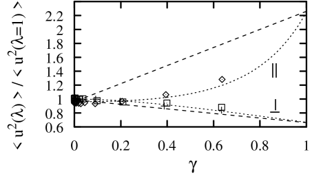
FIG. 1.: Excitation of constrained modes parallel and perpendicular to the elongation at $\lambda=1.5$ as a function of the mode degree of confinement $0\leq\gamma\leq 1$. The dashed (dotted) lines show the predictions eq 33 of Model A and eq 38 of Model B respectively for generalized Rouse modes of a phantom network with identical connectivity. The symbols represent the result of computer simulations of defect-free model polymer networks. [14] The investigated modes are single-chain Rouse modes for network strands of length $N\approx 1.25N_{e}$.

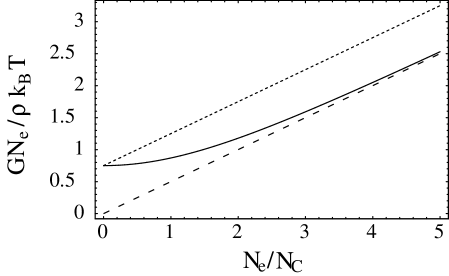
FIG. 2.: Langley plot of the shear modulus. The solid line corresponds to the “double tube” model, the dotted line to the Heinrich–Straube/ Rubinstein–Panyukov model and the dashed line to the phantom model. $N_{e}$ represents the entanglement length and $N_{c}$ the crosslink length.

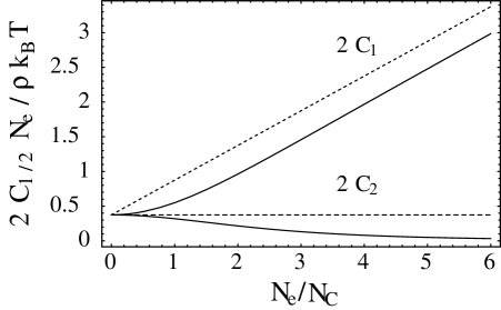
FIG. 3.: Plot of the parameters $2C_{1}$ and $2C_{2}$ of the Mooney-Rivlin equation $f\left(\lambda^{-1}\right)=2C_{1}+2C_{2}\lambda^{-1}$ for the Rubinstein–Panyukov model (dotted) and the “double tube” model (solid).

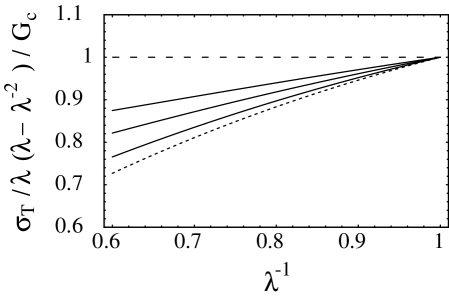
FIG. 4.: Mooney-Rivlin representation of the reduced force for different values of $\Phi$ (from top to bottom: the Phantom model (dashed line, $\Phi=0$), the “double tube” model (solid lines, $\Phi=\frac{1}{3},\frac{1}{2},\frac{3}{4}$) and the Heinrich-Straube/ Rubinstein-Panyukov model (dotted line, $\Phi=1$)).

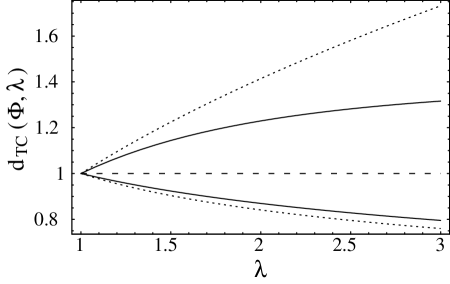
FIG. 5.: Tube diameter $d_{TC}(\Phi,\lambda)=\left((1-\Phi)+\frac{\Phi}{\lambda^{2}}\right)^{-\frac{1}{4}}$ in parallel (upper curves) and perpendicular stretching direction for different elongation ratios $\lambda$ whereas $\Phi$ can be expressed by the entanglement length $N_{e}$ and the crosslink length $N_{c}$ by $\Phi=\frac{d_{TC}^{4}}{d_{TB}^{4}}=\frac{1}{1+\left(\frac{N_{e}}{N_{c}}\right)^{2}}$ using $\frac{d_{TB}^{2}}{d_{TA}^{2}}=\frac{N_{e}}{N_{c}}$. The dashed curve corresponds to the Warner–Edwards model, i.e. $d_{TC}(\Phi=0,\lambda)$, the dotted curve corresponds to the Heinrich–Straube/ Rubinstein–Panyukov model, i.e. $d_{TC}(\Phi=1,\lambda)$, and the solid line represents the “double tube” model with $\Phi=\frac{3}{4}$.

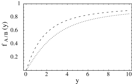
FIG. 6.: Comparison of the universal scaling functions of eqs 66, 74 for the Warner-Edwards model (dashed) and the Heinrich–Straube/ Rubinstein–Panyukov model (dotted) with $y=\frac{R_{g}^{2}|x-x^{\prime}|}{d_{TA/B}^{2}}$.

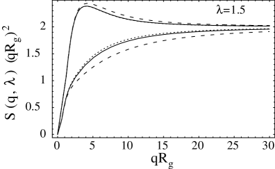
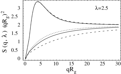
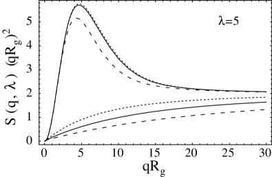
FIG. 7.: Kratky plots of the different structure factors in parallel and perpendicular stretching direction with $\frac{R_{g}}{d_{T}}=6$: Warner–Edwards model (dashed), Heinrich–Straube/ Rubinstein–Panyukov model (dotted line), “double tube” model with $\Phi=\frac{3}{4}$ solid line). The upper curves correspond to the perpendicular stretching direction.

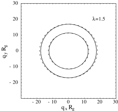
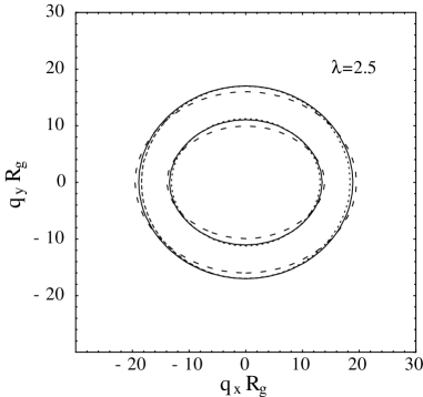
FIG. 8.: Contour plots of the different structure factors with $\frac{R_{g}}{d_{T}}=6$: Warner–Edwards model (dashed), Heinrich–Straube/ Rubinstein–Panyukov model (dotted line), “double tube” model with $\Phi=\frac{3}{4}$ (solid line). The upper curves correspond to the perpendicular stretching direction.

REFERENCES

- [1] Treloar, L. R. G. The Physics of Rubber Elasticity; Clarendon Press: Oxford, 1975.
- [2] Doi, M.; Edwards, S. F. The Theory of Polymer Dynamics; Claredon Press: Oxford, 1986.
- [3] Flory, P. J. J. Chem. Phys. 1949, 17, 303.
- [4] James, H. J. Chem. Phys. 1947, 15, 651.
- [5] James, H.; Guth, E. J. Chem. Phys. 1947, 15, 669.
- [6] Flory, P. J. Proc. Royal Soc. London Ser. A. 1976, 351, 351.
- [7] Mezard, M.; Parisi, G.; Virasoro, M. V. Spinglas Theory and Beyond; World Scientific: Singapore, 1987.
- [8] Edwards, S. F. Proc. Phys. Soc. 1967, 91, 513.
- [9] Edwards, S. F. J.Phys. A 1968, 1, 15.
- [10] Deam, R. T.; Edwards, S. F. Phil. Trans. R. Soc. A 1976, 280, 317.
- [11] Eichinger, B. E. Macromolecules 1972, 5, 496.
- [12] Higgs, P. G.; Ball, R. C. J. Phys. (France) 1988, 49, 1785.
- [13] Zippelius, A.; Goldbart, P.; Goldenfeld, N. Europhys. Lett. 1993, 23, 451.
- [14] Everaers, R. New J. Phys. 1999, 1, 12.1-12.54.
- [15] Warner, M.; Edwards, S. F. J.Phys. A 1978, 11, 1649.
- [16] Ronca, G.; Allegra, G. J. Chem. Phys. 1975, 63, 4990.
- [17] Flory, P. J. J. Chem. Phys. 1977, 66, 5720.
- [18] Erman, B.; Flory, P. J. J. Chem. Phys. 1978, 68, 5363.
- [19] Flory, P. J.; Erman, B. Macromolecules 1982, 15, 800.
- [20] Kästner, S. Colloid Polym. Sci. 1981, 259, 499 and 508.
- [21] Edwards, S. F. Proc. Phys. Soc. 1967, 92, 9.
- [22] Marrucci, G. Macromolecules 1981, 14, 434.
- [23] Graessley, W. W. Adv. Pol. Sci. 1982, 47, 67.
- [24] Gaylord, R. J. J. Poly. Bull. 1982, 8, 325.
- [25] Heinrich, G.; Straube, E.; Helmis, G. Adv. Pol. Sci. 1988, 85, 34.
- [26] Edwards, S. F.; Vilgis, T. A. Rep. Progr. Phys. 1988, 51, 243.
- [27] de Gennes, P. G. J. Chem. Phys. 1971, 55, 572.
- [28] Duering, E. R.; Kremer, K.; Grest, G. S. Phys. Rev. Lett. 1991, 67, 3531.
- [29] Duering, E. R.; Kremer, K.; Grest, G. S. J. Chem. Phys. 1994, 101, 8169.
- [30] Everaers, R.; Kremer, K. Macromolecules 1995, 28, 7291.
- [31] Straube, E.; Urban, V.; Pyckhout-Hintzen, W.; Richter, D. Macromolecules 1994, 27, 7681.
- [32] Straube, E.; Urban, V.; Pyckhout-Hintzen, W.; Richter, D.; Glinka, C. J. Phys. Rev. Lett. 1995, 74, 4464.
- [33] Westermann, S.; Urban, V.; Pyckhout-Hintzen, W.; Richter, D.; Straube, E. Macromolecules 1996, 29, 6165-6174.
- [34] Read, D. J.; McLeish, T. C. B. Phys. Rev. Lett. 1997, 79, 87.
- [35] Read, D. J.; McLeish, T. C. B. Macromolecules 1997, 30, 6376.
- [36] Westermann, S.; Urban, V.; Pyckhout-Hintzen, W.; Richter, D.; Straube, E. Phys. Rev. Lett. 1998, 80, 5449.
- [37] Read, D. J.; McLeish, T. C. B. Phys. Rev. Lett. 1998, 80, 5450.
- [38] Gottlieb, M.; Gaylord, R. J. Polymer 1983, 24, 1644.
- [39] Gottlieb, M.; Gaylord, R. J. Macromolecules 1984, 17, 2024.
- [40] Gottlieb, M.; Gaylord, R. J. Macromolecules 1987, 20, 130.
- [41] Erman, B.; Monnerie, L. Macromolecules 1989, 22, 3342.
- [42] Kloczkowski, A.; Mark, J.; Erman, B. Macromolecules 1995, 28, 5089.
- [43] Rubinstein, M.; Panyukov, S. Macromolecules 1997, 30, 8036.
- [44] Everaers, R. Eur. J. Phys. B 1998, 4, 341.
- [45] Graessley, W. W. Macromolecules 1975, 8, 186 and 865.
- [46] Kloczkowski, A.; Mark, J.; Erman, B. Macromolecules 1992, 23, 3481.
- [47] Sommer, J. U.; Schulz, M.; Trautenberg, H. L. J. Chem. Phys. 1993, 98, 7515.
- [48] Shy, L. Y.; Eichinger, B. E. J. Chem. Phys. 1989, 90, 5179.
- [49] Higgins, J. S.; Benoit, H. C. Polymers and Neutron Scattering; Claredon Press: Oxford, 1997.
- [50] des Cloizeaux, J. Journal de Physique (France) 1994, 4, 539.
- [51] Ullman, R. J. Chem. Phys. 1979, 71, 436.