Firm Diversification and the Law of Proportionate Effect

Abstract

The paper presents an analysis performed over the worldwide top $150$ firms in the pharmaceutical industry. It begins with a test of the Gibrat’s Law of Proportionate Effect finding, in line with previous literature, a violation concerning the variance of the growth. Then it shows, using disaggregated data on sub-markets (defined according to the ATC code) that this violation can be completely referred to the existence of a “diversification” effect, namely a scale relation between the number of active sub-markets a firm posses and its size. The observed scaling property of the firms diversification patterns is in contrast with the linear assumption typically made in literature. Finally, to interpret the findings, the work proposes a stochastic model for firms diversification which fits quite well the data.

1 Introduction

In industrial economics the “stochastic” approach to the description of firms behavior has been introduced long ago with the advent of the Gibrat’s “random walk” description of the business firm growth process (Gibrat (1931); for an historical review see Sutton (1997)). Although this kind of analysis has been applied to the study of the time evolution of firms “size” (measured by diverse variables like sales or employees) with a certain degree of success, the persistent lack of data has prevented its application to other firm-specific relevant economic variables (as productivity, profitability or diversification, to cite a few).

Moreover, the assumption of “identity” between the “objects” (firms) that form the system (industry or sector) implicit in the “statistical” description, while perfectly natural in contexts like biology, ecology or physics, where the “stochastic” models have found a large domain of application, seemed to many authors dissatisfying if applied to the description of economic phenomena. In fact, a large mainstream literature seems going exactly in the opposite direction, trying to characterize industry dynamics starting from a set of firm-specific characteristics (both observable, as the firm’s age Mueller (1972) or unobservable, as its “state” inside a “natural” growth cycle Greiner (1972)). These models, contrary to the “stochastic” ones, typically concentrate on variables, like productivity or profitability, considered more relevant to describe the actual firm “performance”. It must be noted, however, that even if these studies can be used to obtain “interpretative guidelines” (see for instance Dosi et al. (1995)) they would need, in order to be (dis)proved or at least completely exploited in their descriptive power, datasets far more complete that the ones available today.

The present contribution can be considered halfway between the two previous approaches. Indeed, while it is based on “stochastic modeling” which, with its high degree of “essentiality”, has proved to be a powerful tool for an empirical based analysis of firms size dynamics, it extend such technique to an other, in same sense more “strategic”, aspect of firms behavior constituted by their diversification patterns. In this sense it constitutes a first attempt to include, via an empirical grounded analysis, relevant firm-specific economic variables in the description of firm growth performances.

The baseline model in stochastic firms growth dates back to the pioneering work of Gibrat who proposed a model, known as “Law of Proportionate Effect” (LPE), relating the size of a firm and its rate of growth by the expression

$$S(t+1)=S(t)\left(1+R(t)\right)$$ (1)

where $S(t)$ is the firm’s size at time $t$ and $R$ is a random variable not dependent on $S$. This process reduces to a random walk in the log of size $s(t)=\log(S(t))$ and (under the usual assumption of validity of the Central Limit Theorem) predict an asymptotic log - normal size distribution. This “crude” model misses many important aspects of industrial dynamics (firms entry, exit, merging, etc.) and various refinements have been proposed (as an example see Hart (1962), Simon and Bonini (1958), Ijiri and Simon (1977), Sutton (1998) and recently Gerosky (1999)) but it provides a robust framework for the interpretation of data. From its introduction the LPE has been empirically tested by many authors on different and heterogeneous datasets (for a recent review see Sutton (1997)) generally obtaining two, in some sense opposite, conclusions: the Gibrat hypothesis is confirmed in first approximation by the lack of any relationship between the (log) size of firms and their rate of growth but is violated by a clear dependence of the growth variance on size (see, for instance Evans (1987); Hall (1987); Mansfield (1962) and more recently Stanley et al. (1997); Lee et al. (1998)).

A natural explanation for the reduction of growth variance with size could be a sort of “portfolio” effect (see eg. Hymer and Pashigian (1962)). The basic idea is that a firm can be described as a collection of “atomic” components (line of productions, plants, etc.) of roughly the same size whose number would be proportional to the size of the firm. Under the assumption that the growth processes for different components are independent, the Law of Large Number (LLN) would predict a linear relationship between the firm size and the variance of its growth rate. The observed dependence is however milder and the failure of the LLN is usually inputed (see e.g. Boeri (1989)) to the existence of a “relation” between the firm components that makes the aggregation of the “atomic” growths not simply additive A model has recently been proposed Stanley et al. (1997); Lee et al. (1998), based on a supposed intra-firm complex hierarchical structure, which, opportunely tuned, reproduce quite well the observed behavior. On the contrary, I will show in what follows that, if one correctly identifies the “atomic” contributions to growth and the scaling relation between their number and the firm size, the LLN does a good job in explaining the observed Gibrat violation, at least as far as the database under analysis is concerned, without any need of intra-firm “structure”.

The analysis presented in the following is based on the dataset PHID (Pharmaceutical Industry Database) that covers the top $100$ firms relative to the seven major western markets (USA, United Kingdom, France, Germany, Spain, Italy and Canada) in the period ranging from $1987$ to $1997$. The dataset provides the firms sales in USD, disaggregated up to the 4-digit-level of the Anatomical Therapeutic Classification scheme (ATC) in 517 micro classes.

The firms under analysis are obtained aggregating the regional figures and merging from the beginning the sales pertaining to firms that belong to the same entity at the end of period. Moreover, I consider only the $150$ so obtained firms with the top sales at the beginning of the period.

Figure 1: Moments of the $g$ distribution computed at different times

In the next section I present a brief overview of the statistical properties of the size distribution and of the growth process. A wider analysis is presented in Bottazzi et al. (2000), here I concentrate the attention on the violation of the Gibrat model emerging as a relation between the variance of growth and the size of a firm. In Section 3, I perform a deeper analysis of this relation, using disaggregate data on the “sub-markets” defined by the 4-digit ATC code. I am then able to reduce the Gibrat violation to a “diversification” effect, due to a scale relationship between the firm size and the number of its active markets. Finally in Section 4, I propose a model, inspired by the structure of the “technological evolution” in the pharmaceutical industry, which accounts for the observed pattern of firm’s diversification.

2 Data analysis

Figure 2: Distribution function for the firm “normalized size” $g$. The three curves correspond to the distribution obtained for $t=0,5,10$.

Let $S_{i}(t)$ be the size of firm $i$ ($i\in[1,\ldots,N]$) at time $t$ ($i\in[0,\ldots,T]$) where (see Sec. 1) $N=150$ and $T=10$ and let define the ‘normalized sizes” as $G_{i}(t)=S_{i}(t)/<S_{i}(t)>$. This variable and its log $g_{i}(t)=\log(G_{i}(t))$ are characterized by distribution functions that can be considered stationary in time. The reliability of this assumption can be checked plotting the moments of the distribution as a function of time (see Fig. 1): a part from a constant mild increase in the variance of the distribution, the approximation turns out to be good. However the major contribution to the variance increase comes clearly from the low $g$ region ( see Fig. 2) where a “spurious” (due to the selection bias) diffusion toward smaller sizes is present. This diffusion is responsible for the observed increase in variance. Once understood, this effect is statistically irrelevant and in the following analysis the $g$ variable is thought identically distributed at every time step.

As a first step in the search for a violation of the LPE it is natural to investigate the possible presence of a relation between the first moments of the growth distribution and the size. One can proceed in a straightforward way: said $h_{i}(t)=g_{i}(t+1)-g_{i}(t)$ the growth of firm $i$ at time $t$, one bins all the firm according to their size $g_{i}(t)$ in equally numbered sets, and computes the mean, standard deviation and $1$-lag autocorrelation of the growth $h_{i}(t)$ for each set separately. The results are reported in Fig. 3 against the average size of each bin.

Both the mean growth and the autocorrelation do not show any particular pattern but a clear dependence of the growth variance on size emerges and The Law of Proportionate Effect is violated. Fitting the relation between variance of growth and size with an exponential law

$$\sigma(h)\sim e^{\beta g}$$ (2)

one find a value $\beta=.2+-.03$ that is striking similar to the one found in other analysis on different datasets Stanley et al. (1997) Lee et al. (1998) and much lower then the “portfolio” prediction $\beta=.5$ discussed in Sec. 1.

In what follows I will show that the LLN is, however, sufficient to completely characterize the relation in (2). The key point will be to look at the whole firm growth as an “aggregation” of its growth in the different sub-markets in which it operates.

3 Diversification as a source of Gibrat violation

Figure 3: Mean, standard deviation and autocorrelation of growth $h$ computed for different size bins plotted against the average size in the bin. The exponential fit to the standard deviation gives a value $\gamma=-0.20+/-0.03$

One of the peculiar feature of the PHID database is the possibility of disaggregate the sales figures until the $4$th digit of the ATC code. This level of disaggregation allows to identify sub-markets that are “specific” enough to be considered, roughly speaking, the loci of competition between firms: the products belonging to a given sub-market posses similar therapeutic characteristics and can then be considered substitutable while products belonging to different sub-markets are usually targeted to different pathologies. Moreover, the data on licensing agreements Orsenigo et al. (2000) show that this disaggregation level is also the one at which single research projects develop. These characteristics lead to the conclusion that the different “therapeutic sub-markets” provide the natural “scale” at which the “firm’s growth” phenomenon must be studied.

The analysis in this section is limited to the variance-size relation characterizing the growth process of firms. It turns out that the Law of Large Number is in fact responsible for this effect if one assumes as “atomic” contribution to the firm’s growth the growth of firm’s sales in the different sub-markets. This result comes from two non-trivial observations: first, correlation across sub-market is negligible and second, the number of active sub-markets of a given firm is on average increasing with its size.

To make the argument clearer, let me introduce a bit of notation. Let $S_{i,j}(t)$ be the size of firm $i$ in sub-market $j$ at time $t$. The aggregate size of the $i$-th firm is the sum of its size on all the sub-market $S_{i}(t)=\sum_{j}S_{i,j}(t)$ and the aggregate growth defined in (1) can be rewritten as

$$R_{i}(t)+1=\frac{S_{i}(t+1)}{S_{i}(t)}=\sum_{j}\frac{S_{i,j}(t+1)}{S_{i}(t)}\,.$$ (3)

If one computes the correlation of the ratios $S_{(i,j)}(t+1)/S_{i}(t)$ for all the firms in all the sub-markets, i.e. among all the possible couples of indeces $i$ and $j$, one obtains a distribution centered around zero. The growth processes on different sub-markets can be considered to any extent uncorrelated and the variance of the aggregate growth is obtained adding the variance of the growth in each sub-market.

Figure 4: Results of various statistics computed on groups of firms binned according to their size. On the $x$-axis is the log of the average size of the bin. (a) Mean and (b) variance of $R_{i,j}(t)$ for different sub-markets $j$. (c) Mean and (d) variance of $\Delta_{i,j}(t)$ for different sub-markets $j$.

In order to keep the present analysis consistent with the results of previous Sections it is necessary to switch to the “rescaled size” $G_{i}(t)$. This can be done straightforwardly but for clarity purposes let me introduce the new variables $R_{i,j}(t)=S_{i,j}(t+1)/S_{i,j}(t)$ and $\Delta_{i,j}(t)=N_{i}(t)\,S_{i,j}(t)/S_{i}(t)$ where $N_{i}(t)$ is the number of sub-markets in which firm $i$ operates at time $t$ (active sub-markets). Then using (3) the variance of the “normalized growth” can be written as

$$\mbox{var}_{i,t}[H_{i}(t)]=\mbox{var}_{i,t}\left[\frac{G_{i}(t+1)}{G_{i}(t)}\right]=\sum_{j}\mbox{var}_{i,t}\left[\frac{M(t)}{M(t+1)}R_{i,j}(t)\frac{\Delta_{i,j}(t)}{N_{i}(t)}\right]$$ (4)

where $M(t)$ is the average (aggregate) size of firms at time $t$ and the ratio $M(t)/M(t+1)$ is a normalization factor (proportional to the rate of growth of the total industry). I used the short notation $\mbox{var}_{i,t}$ to denote the variance of the distribution obtained, consistently to what done in previous Sections, using the complete panel (all the firms at all the time steps).

In (4) the contribution of each sub-market factorizes in three terms: $R_{i,j}(t)$, which is the actual growth of the firm $i$ in sub-market $j$; the inverse number of active markets $1/N_{i}(t)$ and $\Delta_{i,j}(t)$, which is a weighting coefficient describing the “diversification” heterogeneity of a firm: if the firm $i$ at time $t$ is symmetrically diversified over its sub-markets, the $\Delta_{i,j}(t)$ (for different $j$) are concentrated around $1$, otherwise if the firm is asymmetrically diversified, the $\Delta_{i,j}(t)$ are broadly distributed. The mean and variance of the distributions for $R_{i,j}(t)$ and $\Delta_{i,j}(t)$ obtained using different bins in the aggregate size do not show any clear dependence on the average size of the bin (see Fig. 4). Then the term $N_{i}(t)$, the number of active sub-market a firm posses, must be the sole responsible for the observed dependence of variance over the aggregate size. Indeed, fitting on a log-log scale the average number $<N_{i}(t)>$ of active markets for each bin against the average size of the bin (see Fig. 5) one obtains a slope $\alpha=.39+-.02$ and an intercept $q=6+-0.12$. The Law of Large Number would predict a relation between the exponent in (2) and the slope in Fig. 5 of the form $\beta=-\alpha/2$ which is in perfect agreement with the data.

The conclusion is that the relation provided by the Law of Large Number is valid as long as one consider the actual number of sub-markets a firm operate in. It must be stress, however, that in order to demonstrate this statement, it has been necessary to rule out two possible sources of functional dependence between a firm’s size and the variance of its aggregate growth: the possibility that the variance or the mean of a firm growth in a given sub-market depend (on average) on its total size and the possibility that the diversification patter of a firm (described by the variable $\Delta_{i}$) varies (on average) with its size. Both these possibilities are actually discussed in literature Hart and Prais (1956) and proposed as possible source of Gibrat Law violation.

Figure 5: Average number of active sub-markets. The fit is a straight line with slope $\alpha=.39+-.02$ and intercept $q=6.0+-0.12$

It remains however to explain why the number of active markets a firm possesses, shows a so clear dependence on its size $N(G)\sim G^{\lambda}$ and what is the meaning (if any) of the parameter $\lambda$. In the next Section I propose a model for the diversification process of business firms, essentially based on the assumption of a “self-reinforcing” effect concerning the “proliferation” of sub-markets a firm operates in, which provide a simple but suggestive interpretation of Fig. 5.

4 A stochastic branching model for firm diversification

The previous analysis shows that larger firms are present, on average, on a greater number of sub-markets. For the purposes of this Section it is useful to read this statement in a “dynamical” way: as firms grow their activities becomes more and more diversified as they sell products on different sub-markets.

In what follows I will try to capture the diversification “behavior” of firms with a model describing how the number of active markets (or better, the probability of having a given number of active markets) changes as firm grows. Notice that I’m not interested in a “dynamical” process in time, i.e. a model describing the evolution of diversification structure “as time goes by”. This is because the growth dynamics of the same firm could be very heterogenous if observed at different time steps (actually, in this sector, it is, see.Bottazzi et al. (2000)) and it would be difficult to maintain that shrinking firms behave, with respect to diversification, as growing ones. Rather, I will treat some “size” variable as independent and describe the change in diversification patterns as this quantity is varied. Due to the multiplicative nature of the growth, the natural candidate to play the usual role of “time” is the log of firms size $g$. The object of the following analysis thus becomes the probability that a firm which possesses $n$ active markets when its (log) size is $g$, will possess $m$ active markets when its (log) size is $g^{\prime}\geq g$, $P(n,g;m,g^{\prime})$.

Before proceeding with the model building, let me briefly mention a collection of models that can be considered a previous attempt to merge both the “diversification” and the “growth” aspect of firm’s dynamics. These models, collectively referred as “island models”, was originally proposed by Simon (see Ijiri and Simon (1977)), and can be considered a “classic” in the stochastic growth theory of firms There the “diversification” dynamics is not directly analyzed, but rather serves as a “driving” process that “sets the pace” for the firms growth process, described as a successive capture of diverse “islands”, or “business opportunities”. In this way the distinction between “growth” and “diversification” becomes rather vague, but nevertheless two assumptions seem to be generally accepted concerning the latter. The first is on the nature of the “diversification” events (here the entry on either a previously unexplored or unexploited market): according to it, these events are seen as “shocks” (investment opportunities, technological achievements, etc.) that can “happen” to firms along their histories with mutual independence. The second is to consider these “shocks” uncorrelated in time. i.e. to assume that they could happen with the same constant probability in any instant, irrespectively to the actual firm “state”. If one neglects the possibility of “instantaneous” multiple shocks, the previous assumptions provide a complete definition of the transition probability $P(n,g;m,g+\delta)$ between two sizes differing by an infinitesimal quantity $\delta$:

$$P(n,g;m,g+\delta)=\left\{\begin{array}[]{ll}\lambda\,\delta+o(\delta)&m=n+1\\ o(\delta)&m>n+1\end{array}\right.\;\;\;.$$ (5)

where $\lambda$ is the constant “shock rate” (the average number of “diversification events” for unit time); this form of the transition probability defines the well known Poisson process. A pictorial illustration of this process is shown in Fig. 7: the “blobs” stand for the diversification event “black boxes” that a firm meets along its growth. As far as this model is concerned, it is irrelevant what really happens inside the back box, what matters is that after the “shock” the firm ends with one more active sub-market.

Figure 6: Diversification by independent events. The interarrival “times” $s_{i}-s_{i_{1}}$ are exponentially distributed.

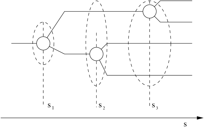
Figure 7: Diversification by branching. The interarrival “times” are no longer exponential, the distance between two events decreases as the number of active markets increases.

The Poisson process would however predict a linear increase of the average number of active sub-markets with $g$, a property that is clearly in contrast with the empirical results discussed in the previous Sections. In order to obtain a more satisfying model, it proves to be useful to explore inside the “black boxes” of Fig 7, and try to describe, at least partially, the actual nature of the diversification events. A possible interpretation of these events comes from the knowledge about the “technological” behavior of the industry Orsenigo et al. (2000). The growth in pharmaceutical industry is highly “research driven” so that it is plausible to think to the diversification too as an outcome of “technical improvements”: a firm enters a new market when it has the (technical) capability of developing products for this market. Moreover previous studies over a wide set of patent agreements Orsenigo et al. (2000) showed that, for what concerns this sector, the technical knowledge proceeds with successive refinements with new results bringing in new possibilities of technological advancements. Then, the simplest way of mapping the resulting “technological behavior” on the diversification dynamics is to suppose that the diversification process proceed as a branching process, where each opened branch (sub-market) becomes eventually the origin of a new branching (diversification) event. A picture of this process is shown in Fig. 7 under the (minimal) assumption that the branching is uniformly binary. If one neglects the topology in sub-markets space that emerges from these successive branchings, but is interested only in the actual number of these sub-markets, the process in Fig. 7 can be readily described: all the active sub-markets can be sources of a possible “diversification” event “à la” Poison, and the (5) must be modified to read

$$P(n,g;m,g+\delta)=\left\{\begin{array}[]{ll}n\,\lambda\,\delta+o(\delta)&m=n+1\\ o(\delta)&m>n+1\end{array}\right.$$ (6)

where again multiple instantaneous branchings are neglected. If $p_{n}(g)$ is the probability that a firm of size $g$ has $n$ active markets it must satisfy the (pure-birth) set of equations

$$\begin{array}[]{lclr}p_{n}(g+\delta)&=&p_{n-1}(g)\,P(n-1,g;n,g+\delta)-p_{n}(g)\,P(n,g;n,g+\delta)&n>n_{0}\\ p_{n_{0}}(g+\delta)&=&-p_{n_{0}}(g)\,P(n_{0},g;n_{0},g+\delta)&n=n_{0}\end{array}$$ (7)

where $n_{0}$ is the initial number of active markets. Substituting in (7) the definition given in (6) and taking the limit $\delta\to 0$ one obtains the set of differential equations:

$$\begin{array}[]{lclr}p_{n}^{\prime}(g)&=&-n\,\lambda\,p_{n}(g)+(n-1)\,\lambda\,p_{n-1}(g)&n>n_{0}\\ p_{n_{0}}^{\prime}(g)&=&-n_{0}\,\lambda\,p_{n_{0}}(g)&n=n_{0}\end{array}$$ (8)

with the initial conditions:

$$p_{n}(g_{0})=\left\{\begin{array}[]{l}1,\;n=n_{0}\\ 0,\;n\neq n_{0}\end{array}\right.$$ (9)

where $g_{0}$ is the initial size of the firm. The previous process is known as the Yule process and has been originally proposed to explain the proliferation in time of animal species (for a discussion see Feller (1968) and reference therein). The system (8) can be easily solved (see Appendix 1) to obtain the following distribution:

$$p_{n}(g)={n-1\choose n-n_{0}}\,e^{-n_{0}\lambda(g-g_{0})}\,\left(1-e^{-\lambda(g-g_{0})}\right)^{n-n_{0}}\;,$$ (10)

defined for $g\geq g_{0}$ and $n\geq n_{0}$.

Let me turn now to the problem of describing the observed data with the proposed model. The distribution in (10) contains three parameters: the “diversification” rate $\lambda$, the initial number of active sub-markets $n_{0}$ and the initial firm size $s_{0}$. Since it correctly predicts an exponential increase in the average number of active markets with size

$$<N(g)>=\sum_{n=n_{0}}np_{n}(g)=n_{0}e^{\lambda(g-g_{0})}\;,$$ (11)

one can use the linear fit shown in Fig. 5 to obtain an estimate of the parameters in (11), requiring the fulfillment of the two conditions $\lambda=\alpha=.39$ and $\log(n_{0})-\lambda s_{0}=q=-6$.

The descriptive power of the model, however, must be judge using more distinguishing object than the average $<N(s)>$. A good candidate is the diversification pattern of the whole industry. To be precise, let $P(M_{0}<M<M_{1})$ be the probability that a firm posses a number of active market between $M_{0}$ and $M_{1}$. This quantity can be evaluated using the actual frequency of occurrences:

$$P^{ob}(M_{0}<M<M_{1})=\frac{1}{TN}\sum_{m=M_{0}}^{M_{1}}\sum_{i=1}^{N}\sum_{t=0}^{T-1}\delta(n_{i}(t)-m)$$ (12)

where $n_{i}(t)$ is the number of active market of firm $i$ at time $t$ and $\delta$ is the Kronecker delta. There is, however, an alternative approach for the computation of the previous quantity: it can be obtained via a simple convolution

$$P(M_{0}<M<M_{1})=\sum_{m=M_{0}}^{M_{1}}\int_{g_{0}}^{+\infty}dgf(g)\,p_{m}(g)$$ (13)

once the size probability density $f(s)$ and the “diversification” probability $p_{n}(g)$ are known. An estimate of (13) can be obtained using the observed frequencies in data

$$P^{th}(M_{0}<M<M_{1})=\frac{1}{TN}\sum_{m=M_{0}}^{M_{1}}\sum_{i=1}^{N}\sum_{t=0}^{T-1}p_{m}(g_{i}(t))$$ (14)

where $g_{i}(t)$ is the size of firm $i$ at time $t$. Notice that this second method depends on the “branching” model to obtain an estimate of the probabilities $P(M_{0}<M<M_{1})$. A comparison between the observed $P^{ob}$ and the predicted $P^{th}$ distributions provides a way to tune the residual degree of freedom, and an indication of the goodness of the model. As showed in Fig. 8 the accordance, considering the extreme simplifications introduced, is good.

Figure 8: The binned probability density for the number of sub-market computed directly by the data and theoretically predicted by the Yule process. The fit showed was obtained with $\lambda=.39$, $n_{0}=5$ and $s_{0}=-12$. As comparison, a fit of a Poisson model with a non linear intensity function $\tau(G)=G^{\lambda}$ is also shown.

5 Conclusions and outlook

The relation between the variance of growth and the size, which constitutes the clearest and often reported violation of the Gibrat law has been reduced to a diversification effect: bigger firms operate in more sub-markets and the variance of their growth is consequently reduced. I have shown that, in the industry under analysis, other possible effects (in particular the correlation among sub-markets and the dependence of the “strategic” diversification pattern of a firm on its size) if exist, are negligible.

The actual structure of the firm diversification can be described with good accuracy using the simple stochastic process proposed in Sec. 4. A caveat must be introduced, however, regarding the “interpretation” of this model: the strong technological component in industry growth suggests, but does not imply, that the main driving force in diversification would be some sort of “technological specification”. The “penetration” of a firm in a new sub-market can actually possess various natures, nevertheless the proposed model is likely to describe the diversification dynamics irrespectively of this variety. The reasons of this flexibility are in the simplicity of the hypotheses. The model is indeed based on two general assumptions: first, the existence of some sort of “competencies” providing the firm with the ability to diversify its business, and second, that these “competencies” (and so the ability to enter a new sub-market) increase with the number of times they have been effectively used (and so with the number of opened sub-markets). Both these assumption seem, in most cases, so reasonable that would be difficult to find arguments against them.

The previous model, thus, suggests an “evolutionary” description of firms which progressively “learn” to diversify, whatever the object of this learning would be. Incidentally, the observed relationship between the growth variance and the size of the firms, being milder than the LLN prediction, gives evidence against the interpretation of “diversification” as a risk minimization strategy: indeed if this would be the case, firms have to be present on much more sub-markets then they actually are.

The present analysis can be extended in several directions: the first concerns the generality of the previous findings relating Gibrat’s Law violation to a diversification effect. In Sec. 3 only one industry has been analyzed, but the observed trend in Fig. 3 is so similar to other results in literature (Stanley et al. (1997),Lee et al. (1998)) that a major multi-sectorial investigation, where possible, is advisable. Second, concerning the proposed model of firm diversification, it would be important to empirically investigate the nature of the “competencies” leading to penetration in new markets and their connection with the different characteristics of the firm, the more interesting probably being its “technological advantage”. This investigation would constitute an important empirical support to the construction of evolutionary models of the firm (in line with what has been done, for instance, in Dosi et al. (1995)). Finally, it would be interesting to apply the same description to diversification data from other industries. This would be a test of the model previously described, but, more interestingly, could constitute, via the introduction of industry-specific parameters, a “dynamical” way of characterizing diversification pattern in different sectors.

6 Acknowledgments

The author thanks Giovanni Dosi, Fabio Pamolli and Massimo Riccaboni for helpful comments and useful discussions.

APPENDIX

Appendix A Solution of the Yule process

To simplify the solution of (8) let me introduce a rescaled size $t=\lambda(g-g_{0})$ and consider, instead of the probabilities in (6), the variables $y_{n}(t)$ defined by

$$p_{n}(t)=e^{-nt}\,y_{n}(t)\;.$$ (15)

In these new variables the set of equation in (8) reduces to:

$$\begin{array}[]{lclr}y^{\prime}_{n}(t)&=&(n-1)\,e^{t}\,y_{n-1}(t)&n>n_{0}\\ y^{\prime}_{n_{0}}(t)&=&0&n=n_{0}\;.\end{array}$$ (16)

with initial conditions:

$$y_{n}(0)=\left\{\begin{array}[]{l}1,\;n=n_{0}\\ 0,\;n\neq n_{0}\end{array}\right.$$ (17)

From (16), iterating over the index $n$, it is immediate to write the solution as multiple integral:

$$y_{n}(t)=(n-1)\,(n-2)\ldots n_{0}\,\int_{0}^{t}dt_{1}\int_{0}^{t1}dt_{2}\ldots\int_{0}^{t_{n-n_{0}+1}}dt_{n-n_{0}}e^{t_{1}+t_{2}+\ldots+t_{n-n_{0}}}$$ (18)

Notice that, due to the complete symmetry of the integrand, the multiple integral over the $n-n_{0}$-dimensional hyper-cube of side $t$ with the constraints $t_{n-n_{0}}<\ldots<t_{2}<t_{1}<t$ reduces to the integral over the whole hypercube divided by all the possible ordering of the constraints, which are $(n-n_{0})!$. One thus obtains:

$$y_{n}(t)={n-1\choose n-n_{0}}\,(e^{t}-1)^{n-n_{0}}\;,$$ (19)

that, remembering the factorization in (15) and substituting $t$ with its previous definition, reduces to (10) after obvious algebra.

References

- Boeri (1989) Boeri, T., (1989) “Does Firm Size Matter?”, Giornale degli Economisti e Annali di Economia, 48.
- Bottazzi et al. (2000) Bottazzi G., Dosi G.,Lippi M.,Pammolli F., Riccaboni M., (2000) “Processes of corporate growth in the evolution of an innovation-driven industry” LEM Working Paper, S.Anna Shool.
- Brock (1999) Brock W., (1999) “Scaling in Economics: A Reader’s Guide”, Industrial and Corporate Change, 8(3)
- Dosi et al. (1995) Dosi G., Marsili O., Orsenigo L., Salvatore R., (1995) “Learning, Market Selection and the Evolution of Industrial Structures” Small Business Economics 7:411-436
- Evans (1987) Evans, D., (1987) “Tests of Alternative Theories of Firm Growth’, Journal of Industrial Economics, 95
- Feller (1968) Feller W. (1968) “An Intrduction to Probabilty Theory and Its Applications” Wiley & Sons, N.Y.
- Gerosky (1999) Geroski P. A., (1999), “The Growth of Firms in Theory and Practice”, CEPR working paper 2092, London.
- Gibrat (1931) Gibrat R., (1931) “Les inégalités économiques”, Librairie du Recueil Sirey, Paris.
- Greiner (1972) Greiner L., (1972) “Evolution and Revolution as Organizations grow”, Harvard Business Review, July-August
- Hall (1987) Hall B. H., (1987) “The Relationship Between Firm Size and Firm Growth in the US Manufacturing Sector”, Journal of Industrial Economics, 35, 4
- Hart and Prais (1956) Hart P.E., Prais S. J., (1956) “The Analysis of Business Concentration: A Statistical Approach”, Journal of the Royal Statistical Society, 119, Series A.
- Hart (1962) Hart P., (1962) “The Size and Growth of Firms”, Economica, 29.
- Hymer and Pashigian (1962) Hymer S., Pashigian P., 1962, “Firm Size and Rate of Growth”, Journal of Political Economy, 72, 6, pp. 556-569.
- Ijiri and Simon (1977) Ijiri y., Simon H.A., (1977) “Skew distributions and the sizes of business firms”, North Holland Publishing Company.
- Lee et al. (1998) Lee Y., Nunes Amaral L. A., Canning D., Mayer M. and Stanley H. E. (1998) “Universal Features in the Growth Dynamics of Complex Organizations” Physical Review Letters, n.15, vol.81
- Mansfield (1962) Mansfield D. E., (1962) “Entry, Gibrat’s Law, Innovation, and Growth of the Firms”, American Economic Review, 52, 4
- Mueller (1972) Mueller D., (1972) “A Life Cycle Theory of the Firm”, Journal of Industrial Economics,20
- Orsenigo et al. (2000) Orsenigo L., Pammolli F., Riccaboni M., (2000) “Technological Change and Network Dynamics: Lessons from the Pharmaceutical Industry”, Research Policy, forthcoming; Pammolli F., Riccaboni M., (2000) “Technological paradigms and the nature of markets for technology” proceedings of Workshop On Institutions, Entrepreneurship, and Firm Growth, Jonkoping, Sweden.
- Simon and Bonini (1958) Simon H. and Bonini C., (1958) “The Size Distribution of business Firms”, American Economic Review, 48.
- Sutton (1997) Sutton J., (1997) “Gibrat’s Legacy” Journal of Economic Literature Vol. XXXV
- Sutton (1998) Sutton J., (1998) “Technology and Market Structure, Theory and History”, MIT Press, Cambridge, Ma.
- Stanley et al. (1997) Stanley M. H. R., Nunes Amaral L. A., Buldyrev S. V., Havlin S., Leschhorn, H., Maass P., Salinger M. A., Stanley H. E., (1997) “Scaling behavior in economics: empirical results and modelling of company growth”, Nature, 319.
- Snyder (1975) Snyder D.L. (1975) “Random Point Processes” Wiley & Sons, N.Y.