Investigation of thermodynamic properties of pseudospin-electron model in the gaussian fluctuation approximation

Abstract

A method of consideration of gaussian fluctuations of the effective mean field within the framework of the GRPA scheme is applied to investigation of thermodynamical properties of a pseudospin-electron model (PEM). The grand canonical potential, pseudospin mean value, as well as the mean squares of fluctuations are calculated. Obtained results are compared with corresponding ones obtained by other approximations. An influence of the gaussian fluctuations of mean field on the thermodynamic properties of PEM is discussed.

1 Introduction

The pseudospin-electron model (PEM) was originally proposed to include a local interaction of the conducting electrons in metals (or semimetals) with a certain two level subsystem when it is reasonable to use pseudospin formalism; the pseudospin variable $S_{i}^{z}=\pm 1/2$ defines these two states. Starting from [1, 2] this scheme is applied to describe the strongly correlated electrons of CuO₂ sheets coupled with the vibrational states of apex oxygen ions O_IV (moving in a double-well potential) in YBaCuO type systems. Recently a similar model was proposed for investigation of the proton-electron interaction in molecular and crystalline systems with hydrogen bonds [3, 4]. The model Hamiltonian has the following form:

$$H=\sum_{i}H_{i}+\sum_{ij\sigma}t_{ij}c^{+}_{i\sigma}c_{j\sigma},$$ (1)

and includes, in addition to the terms describing electron transfer ($\sim t_{ij}$), the electron correlation ($U$ - term) in the spirit of the Hubbard model, interaction with the anharmonic mode ($g$ - term), the energy of the tunnelling splitting ($\Omega$ - term), and the energy of the anharmonic potential asymmetry ($h$ - term) in the single-site part

$$H_{i}=Un_{i\uparrow}n_{i\downarrow}-\mu(n_{i\uparrow}+n_{i\downarrow})+g(n_{i\uparrow}+n_{i\downarrow})S^{z}_{i}-\Omega S^{x}_{i}-hS^{z}_{i}.$$ (2)

Based on PEM a possible connection between the superconductivity and lattice instability of the ferroelectric type in HTSC was discussed [2, 5]. Description of the electron spectrum and electron statistics of the PEM was given in [6] within the framework of the temperature two-time Green’s function method in the Hubbard-I approximation.

A series of works has been carried out in which the pseudospin $\left\langle S^{z}S^{z}\right\rangle$, mixed $\left\langle S^{z}n\right\rangle$, and charge $\left\langle nn\right\rangle$ correlation functions were calculated. A possibility of divergences of these functions at some values of temperature exists as it was shown with making use of the generalized random phase approximation (GRPA) [7] in the limit of infinite single-site electron correlations ($U\to\infty$) [8, 9]. This effect was interpreted as a manifestation of dielectric instability or ferroelectric type anomaly. The tendency to form the spatially modulated charge and pseudospin ordering at certain model parameter values was established.

The case of absence of electron transfer ($t_{ij}=0$), but with taking into account of the direct interaction between pseudospins was considered within the mean field approximation [10, 11, 12]. It was shown there that behaviour of the system strongly depends on a thermodynamical regime: at $\mu={\rm const}$ the first order phase transitions with the jumps of pseudospin mean value $\langle S^{z}\rangle$ and electron concentration values $n$ as well as the second ones (with smooth changes) were detected, while at $n={\rm const}$ an instability with respect to phase separation in the electron and pseudospin subsystems can take place.

In the papers [13, 14, 15, 16] PEM was considered at the absence of direct electron-electron interaction and tunnelling splitting ($U=0$, $\Omega=0$). In such a version of PEM (simplified PEM), an effective many-body pseudospin interaction via conducting electrons appears, and hence it is interesting to investigate an influence of the retarded nondirect interaction between pseudospins on thermodynamics of the model. Hamiltonian of this simplified PEM is invariant with respect to the transformation $\mu\rightarrow-\mu$, $h\rightarrow 2g-h$, $n\rightarrow 2-n$, $S^{z}\rightarrow-S^{z}$ (the so-called electron-hole symmetry) what makes possible to describe the hole-pseudospin system as well.

On the other hand, the presented Hamiltonian in the case of absence of electron correlation and tunnelling splitting allows one to describe the binary alloy type model. It is convenient to introduce projective operators on pseudospin states $P^{\pm}_{i}=1/2\pm S^{z}_{i}$; then Hamiltonian of the binary alloy can be obtained by substitution $P^{+}_{i}=p_{i}$, $P^{-}_{i}=1-p_{i}$ where $p_{i}$ is the concentration of one component of binary alloy, and $1-p_{i}$ is the concentration of the second one. Difference between these models is in the way how an averaging procedure over projection operators $P^{\pm}$ is performed (thermal statistical averaging in the case of PEM and configurational averaging for binary alloy) and how the self-consistency is achieved (fixed value of longitudinal field $h$ for PEM and fixed value of the component concentration $p$ for binary alloy).

Furthermore, if in Hamiltonian (1), (2) (considering the simplified case $U=0$, $\Omega=0$), we remove spin indices and rewrite the Hamiltonian in terms of the operators of the mobile $d_{i}$ ($c_{i\sigma}=d_{i}$) and localized $f_{i}$ ($P^{+}_{i}=f^{+}_{i}f_{i}$, $P^{-}_{i}=1-f^{+}_{i}f_{i}$) electrons, we obtain the Hamiltonian of the Falicov-Kimball model where $h$ plays a role of the chemical potential for the localized $f$-electrons. The ground state of the Falicov-Kimball model, when the electron concentration for subsystems is fixed, is not uniform and shows the commensurate or incommensurate ordering or phase separation depending on the concentration and coupling constant values [17]. On the other hand, in the case of the fixed value of field $h$, the bistability effects are observed.

Investigations of the thermodynamic properties of the simplified PEM within the framework of the self-consistent GRPA [13] and dynamical mean field approximation (DMFA) [14] have shown that:

• in the $\mu={\rm const}$ regime (when the electron states of other structure elements, which are not included explicitly into the PEM, are supposed to play a role of a thermostat ensuring a fixed value of the chemical potential $\mu$) the interaction between the electron and pseudospin subsystems leads to the possibility of either first or second order phase transitions between different uniform phases (bistability effect) [13, 14] as well as between the uniform and the chess-board ones [15, 16];

• in the regime $n={\rm const}$ (this situation is more customary at the consideration of electron systems and means that the chemical potential depends now on the electron concentration being the function of $T$, $h$ etc.) an instability with respect to the phase separation in the electron and pseudospin subsystems can take place [13, 14, 16].

The above mentioned methods of investigation of the PEM (within the framework of the self-consistent GRPA scheme as well as within the framework of DMFA in the case of the finite space dimension) take into account only mean field type contributions. It is reasonable only when fluctuation effects are small. In the vicinity of critical points effects of the mean field fluctuations become significant.

The aim of this article is to calculate the thermodynamic and correlation functions of the simplified PEM ($U=0$, $\Omega=0$) within the framework of self-consistent approach, allowing us take into account fluctuation effects of the effective self-consistent mean field. Such a consistent gaussian fluctuation approach was proposed previously in work [18] where expressions for the grand canonical potential and pseudospin correlator as well as a self-consistent set of equations for the pseudospin mean value and root–mean–squares (r.m.s.) fluctuation parameter were obtained.

Furthermore we would like to investigate an influence of the gaussian fluctuations on the thermodynamics of phase transitions in the PEM and discuss an applicability of the schemes previously used for the investigation of the PEM. For this purpose the results of investigation of PEM within the framework of the self-consistent GRPA scheme [13] as well as within the DMFA [14] are presented.

The paper is organized as follows. First, a short review of the self-consistent GRPA approach is presented and the results of the numerical calculations within the framework of this scheme are compared with corresponding ones obtained within the DMFA in [14]. Second, we review the self-consistent gaussian fluctuation approach for the PEM and present its simplified version (analogous to the approximation proposed by Onyszkiewicz [19, 20] for spin models). Then we apply gaussian fluctuation method to investigation of the thermodynamic properties of the PEM, and finally results of the numerical calculations of the pseudospin mean value and r.m.s. fluctuation parameter as well as the grand canonical potential are shown. Phase diagrams are presented and compared to the corresponding ones of the GRPA. Finally, discussion and conclusion are given.

2 Self-consistent GRPA method

We would like to remind that traditional GRPA method (proposed by Izyumov et al. [7] for the investigation of the magnetic susceptibility of the ordinary Hubbard model as well as $t-J$ model) takes into account the same topological class of diagrams (so-called loop diagrams) as in the random phase approximation (RPA). Main difference between the GRPA and RPA is a way of choosing of the basic states: splitted (Hubbard-I) band states in the GRPA method and pure band states in RPA. The question how to calculate thermodynamic quantities within the GRPA has been open until recent works [13, 21]. In this section we briefly show how to construct the mean field type approximation within the GRPA scheme for PEM.

Calculations are performed in the strong coupling case ($g\gg t$) using single-site states as the basic ones. The formalism of electron annihilation (creation) operators $a_{i\sigma}=c_{i\sigma}P^{+}_{i},$ $\tilde{a}_{i\sigma}=c_{i\sigma}P^{-}_{i}$ ($P^{\pm}_{i}=1/2\pm S^{z}_{i}$) acting at a site with the certain pseudospin orientation is introduced [13]. Within the framework of the proposed representation, the initial Hamiltonian (1) (in the case of $U=0$, $\Omega=0$) has the following form:

$$H=H_{0}{+}H_{\rm int}=\sum\limits_{i\sigma}\{\varepsilon_{1}n_{i\sigma}{+}\varepsilon_{2}\tilde{n}_{i\sigma}{-}\frac{h}{2}S^{z}_{i}\}+\sum\limits_{ij\sigma}t_{ij}(a^{+}_{i\sigma}a_{j\sigma}{+}a^{+}_{i\sigma}\tilde{a}_{j\sigma}{+}\tilde{a}^{+}_{i\sigma}a_{j\sigma}{+}\tilde{a}^{+}_{i\sigma}\tilde{a}_{j\sigma}),$$ (3)

where $\varepsilon_{1,2}=-\mu\pm g/2$ are the energies of the single-site states.

Expansion of the calculated quantities in terms of the electron transfer $H_{\rm int}$ leads to the infinite series of terms containing the averages of the $T$-products of the $a_{i\sigma}$, $\tilde{a}_{i\sigma}$, $a^{+}_{i\sigma}$, $\tilde{a}^{+}_{i\sigma}$ operators. The evaluation of such averages is made using the appropriate Wick’s theorem [13] formulated in the spirit of Wick’s theorem for Hubbard operators [22]. This theorem gives an algorithm reducing the average of product of $n$ creation (annihilation) operators to the sum of averages of products of the $n-2$ operators. So it is possible to express the result in terms of the products of nonperturbed Green’s functions and averages of the projection operators $P^{\pm}_{i}$ expanded in semi-invariants.

Nonperturbated electron Green’s function is equal to

$$g(\omega_{n})=\langle g_{i}(\omega_{n})\rangle;\quad g_{i}(\omega_{n})=\frac{P^{+}_{i}}{\rmi\omega_{n}-\varepsilon_{1}}+\frac{P^{-}_{i}}{\rmi\omega_{n}-\varepsilon_{2}}.$$ (4)

In the uniform case $\langle S^{z}_{i}\rangle=\langle S^{z}\rangle$, a single-electron Green’s function (calculated in Hubbard-I type approximation) is $=G_{\boldsymbol{k}}(\omega_{n})$ $=\big{(}g^{-1}(\omega_{n})-t_{\boldsymbol{k}}\big{)}^{-1}$; its poles determine the electron spectrum

$$\varepsilon_{\rm\scriptscriptstyle{I},\rm\scriptscriptstyle{II}}(t_{\boldsymbol{k}})=\frac{1}{2}(-2\mu+t_{\boldsymbol{k}})\pm\frac{1}{2}\sqrt{g^{2}+4t_{\boldsymbol{k}}\langle S^{z}\rangle g+t^{2}_{\boldsymbol{k}}}\,.$$ (5)

Investigation of the electron spectrum was performed in [13]. In this approximation, the branches $\varepsilon_{\rm\scriptscriptstyle{I}}(t_{\boldsymbol{k}})$ and $\varepsilon_{\rm\scriptscriptstyle{II}}(t_{\boldsymbol{k}})$ form two electron subbands always separated by a gap. Reconstruction of the electron spectrum takes place with change of the pseudospin mean value $\langle S^{z}\rangle$.

In the adopted approximation the diagrammatic series for the pseudospin mean value can be presented in the form [13]

$$\langle S^{z}\rangle=\raisebox{-6.82881pt}{\epsfbox{diag02.eps}}\quad,$$ (6)

where the following diagrammatic notations are used: $\raisebox{-3.69899pt}{\epsfbox{diag03.eps}}\,-\,S^{z},$ $\,-\,g_{i}(\omega_{n}),$ wavy line is the Fourier transform of the hopping integral $t_{\boldsymbol{k}}$. Semi-invariants are represented by ovals and contain the $\delta$-symbols on site indices. In the spirit of the traditional mean field approach, renormalization of the basic semi-invariant by insertion of independent loop fragments is taken into account in (6). The analytical expression for the loop is the following:

$$\raisebox{-11.38092pt}{\epsfbox{diag05.eps}}=\frac{2}{N}\sum_{n,\boldsymbol{k}}\frac{t^{2}_{\boldsymbol{k}}}{g^{-1}(\omega_{n})-t_{\boldsymbol{k}}}\left(\frac{P^{+}_{i}}{\rmi\omega_{n}-\varepsilon_{1}}+\frac{P^{-}_{i}}{\rmi\omega_{n}-\varepsilon_{2}}\right)=\beta(\alpha_{1}P^{+}_{i}+\alpha_{2}P^{-}_{i}).$$ (7)

It should be noted that within the presented self-consistent scheme of the GRPA, chain fragments form the single-electron Green’s function in the Hubbard-I approximation, and in the sequences of loop diagrams in expressions for thermodynamic and pair correlation functions the connections between any two loops by more than one semi-invariant are omitted. This procedure includes renormalization of the higher order semi-invariants similar to the one given by expression (6).

Summation of diagrammatic series (6) for the pseudospin mean value is equivalent to averaging with the mean-field type Hamiltonian:

$$H_{\rm MF}{=}\sum\limits_{i}\{\varepsilon_{1}(n_{i\uparrow}{+}n_{i\downarrow})+\varepsilon_{2}(\tilde{n}_{i\uparrow}{+}\tilde{n}_{i\downarrow})-yS^{z}_{i}\},$$ (8)

where an expression $\quad y=h+\alpha_{2}-\alpha_{1}\quad$ determines an internal effective self-consistent field formed by retarded many-body interaction between pseudospins via conducting electrons.

Equation for pseudospin mean value in the uniform case is as follows

$$\langle S^{z}_{l}\rangle=\langle S^{z}\rangle_{\rm MF}=b(y),$$ (9)

where

$$b(y)=\frac{1}{2}\tanh\left\{\frac{\beta}{2}y+\ln{\frac{1+\rme^{-\beta\varepsilon_{1}}}{1+\rme^{-\beta\varepsilon_{2}}}}\right\}.$$ (10)

An analytical expression for mean value of the particle number can be presented in the form [13]:

$$\langle n\rangle=\frac{2}{N}\sum_{\boldsymbol{k}}\Big{[}n(\varepsilon_{\rm\scriptscriptstyle I}(t_{\boldsymbol{k}}))+n(\varepsilon_{\rm\scriptscriptstyle II}(t_{\boldsymbol{k}}))\Big{]}-[1+2\langle S^{z}\rangle]n(\varepsilon_{2})-[1-2\langle S^{z}\rangle]n(\varepsilon_{1}).$$ (11)

Here $n(\varepsilon)=\frac{\displaystyle 1}{\displaystyle 1+\rme^{\beta\varepsilon}}$ is Fermi distribution.

Diagrammatic equation on pseudospin correlator $\langle S^{z}S^{z}\rangle_{\boldsymbol{q}}$ within the framework of the GRPA has the following form:

$$\langle S^{z}S^{z}\rangle_{\boldsymbol{q}}=\raisebox{-17.07182pt}[12.80365pt][19.91684pt]{\epsfbox{diag06.eps}}\quad.$$ (12)

Equation (12) differs from the corresponding one for the Ising model in RPA by the replacement of the direct exchange interaction by the electron loop $\Pi_{\boldsymbol{q}}=\raisebox{-11.38092pt}{ \epsfbox{diag07.eps}}\;$ (describing the many-body retarded interaction between pseudospins via conducting electrons)

$$\Pi_{\boldsymbol{q}}=\frac{2}{N}\sum\limits_{n,\boldsymbol{k}}\Lambda^{2}_{n}\tilde{t}_{n}(\boldsymbol{k})\tilde{t}_{n}(\boldsymbol{k}{+}\boldsymbol{q}),\;\;\Lambda_{n}=\frac{g}{(\rmi\omega_{n}{+}\mu)^{2}{-}g^{2}/4},\;\;\tilde{t}_{n}(\boldsymbol{k})=\frac{t_{\boldsymbol{k}}}{(1-g_{n}t_{\boldsymbol{k}})}.$$ (13)

The first term in equation (12) is the zero-order correlator renormalized due to the inclusion in all basic semi-invariants of the mean-field type contributions (‘single-tail’ parts) coming from the effective pseudospin interaction

(14)

and is thus calculated with the help of Hamiltonian $H_{\rm MF}$.

In analytical form, solution of equation (12) is equal to

$$\langle S^{z}S^{z}\rangle_{\boldsymbol{q}}=\frac{1/4-\langle S^{z}\rangle^{2}}{1+\frac{2}{N}\sum\limits_{n,\boldsymbol{k}}\Lambda^{2}_{n}\tilde{t}_{n}(\boldsymbol{k})\tilde{t}_{n}(\boldsymbol{k}+\boldsymbol{q})(1/4-\langle S^{z}\rangle^{2})},$$ (15)

and is different from zero only in a static case ($\omega_{n}=0$) (since pseudospin operator commutes with the initial Hamiltonian).

Within the same approach the grand canonical potential was obtained [13]. The corresponding analytical expression is

$$\Omega_{\rm GRPA}={-}\frac{2}{N\beta}\sum\limits_{n,\boldsymbol{k}}\ln(1{-}t_{\boldsymbol{k}}g(\omega_{n}))-\frac{2}{N\beta}\sum\limits_{n,\boldsymbol{k}}\frac{g(\omega_{n}))t_{\boldsymbol{k}}^{2}}{g^{-1}(\omega_{n}))-t_{\boldsymbol{k}}}-\frac{1}{\beta}\ln{\Tr}(\rme^{-\beta H_{\rm MF}}).$$ (16)

It was shown that all quantities can be derived from the grand canonical potential

$$\frac{\rmd\Omega}{\rmd(-\mu)}=\langle n\rangle,\quad\frac{\rmd\Omega}{\rmd(-h)}=\langle S^{z}\rangle,\quad\frac{\rmd\langle S^{z}\rangle}{\rmd(\beta h)}=\langle S^{z}S^{z}\rangle_{{\boldsymbol{q}}=0},$$

what demonstrates thermodynamic consistence of the proposed approximation.

In the $\mu=const$ regime the stable states are determined from the minimum of the grand canonical potential. The solution of equation for the pseudospin mean value and calculation of potential $\Omega$ (as well as the pair correlation function) were performed numerically [13]. The first order phase transitions between the different uniform phases (bistability effect) at change of temperature $T$ and field $h$ can take place when chemical potential is placed within the electron subbands. In the case when chemical potential is fixed and placed between the electron subbands, the uniform phase become unstable with respect to fluctuations with $\boldsymbol{q}=(\pi,\pi)$, and the possibility of second order phase transitions between the uniform and chess-board phase exists at the change of temperature or field [16].

As mentioned above, the band structure is determined by the pseudospin mean value (figure 1), and its change is accompanied by the corresponding changes of the electron concentration (see [13, 15] for details).

Figure 1: Field dependences of pseudospin mean value and electron bands boundaries for $\mu=const$ regime when chemical potential is placed in the lower subband (in the self-consistent GRPA) ($g=1$, $t_{\boldsymbol{k}=0}=0.2$, $\mu=-0.5$, $T=0.0132$)

The simplified version of PEM was considered in [14] within the framework of DMFA scheme as well. The obtained phase diagrams within the self-consistent GRPA and DMFA are presented in figure 2 (in the case when chemical potential is placed in the center of lower subband $\mu=-0.5$).

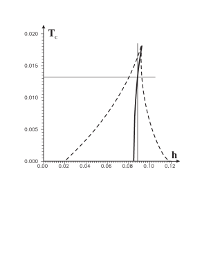
  (a)    (b)

Figure 2: $T_{\rm c}-h$ phase diagrams: (a) within the self-consistent GRPA, (b) within the DMFA [14]. Solid and dashed lines indicate the first order phase transition line and boundaries of the phase stability (spinodal lines), respectively ($g=1$, $t_{\boldsymbol{k}=0}=0.2$, $\mu=-0.5$)

One can see a quite sufficient coincidence of shapes of the first order phase transition curves (thick solid line). But unlike to the phase diagram in figure 2b obtained within the DMFA, boundaries of the phase stability region calculated in the self-consistent GRPA have the same type of slope, hence a region exists, where the vertical line twice crosses the boundary of the phase stability region (figure 2a). The analysis of the $\langle S^{z}S^{z}\rangle$ behaviour in this region (for fixed value of the longitudinal field $h=0.0875$) with the decrease of temperature shows that high temperature phase becomes unstable with respect to fluctuations with $\boldsymbol{q}=0$ (the lower crossing point of the vertical line and boundary of the phase stability region in figure 2a.) Similar results were obtained previously in [8, 9] for temperature behaviour of the correlation functions in the case of infinite single-site electron correlation $U\rightarrow\infty$ within the framework of the GRPA.

In the case of the fixed value of the electron concentration condition of equilibrium is determined by the minimum of free energy. In this regime the first order phase transition with a jump of the pseudospin mean value (accompanied by the change of electron concentration) transforms into a phase separation into the regions with different electron concentrations and pseudospin mean values [13]. For the first time the instability with respect to the phase separation in pseudospin-electron model was marked in [23], where it was obtained within the GRPA in the limit $U\rightarrow\infty$.

3 Self-consistent gaussian fluctuation approximation

The above considered approach takes into account only contributions of mean field type. In this section we present the developed in [18] consistent scheme for calculation of thermodynamic and correlation functions, which takes into account the gaussian fluctuations of the self-consistent mean field. We also reduce the presented here method to more suitable for numerical calculation taking into account a restricted class of diagrams. Such an approximation for spin models with a direct interaction proposed by Onyszkiewicz [19, 20] yields a much better description of critical properties of spin models in the whole range of temperature then others.

In constructing a higher order approximation that takes into account the fluctuation effects of the self-consistent mean field, we use the self-consistent GRPA as the zero-order one. This means that all ‘single-tail’ parts of diagrams (6) and (14) are already summed up and all semi-invariants are calculated using the distribution with the Hamiltonian $H_{\rm MF}$ (8). All these semi-invariants are represented graphically by thick ovals and contain the $\delta$-symbols on site index:

$$\raisebox{-2.56064pt}{\epsfbox{diag09.eps}}{=}\langle S^{z}\rangle_{\rm MF}=b(y),\;\raisebox{-2.56064pt}{\epsfbox{diag10.eps}}{=}\langle S^{z}S^{z}\rangle^{\rm c}_{\rm MF}=\frac{\partial b(y)}{\partial\beta y},\;\raisebox{-2.56064pt}{\epsfbox{diag11.eps}}{=}\langle S^{z}S^{z}S^{z}\rangle^{\rm c}_{\rm MF}=\frac{\partial^{2}b(y)}{\partial(\beta y)^{2}}.$$ (17)

As an approximation that goes beyond of the self-consistent GRPA we use, similarly to [24, 25], the approach taking into account the so-called ‘double-tail’ diagrams. A corresponding diagrammatic series for the pseudospin mean value can be written as

$$\langle S^{z}\rangle=\raisebox{-7.11317pt}[39.83368pt][2.84544pt]{\epsfbox{diag12.eps}}\quad.$$ (18)

The diagrammatic equation for the pseudospin correlator $\langle S^{z}S^{z}\rangle_{\boldsymbol{q}}$ within the presented here approximation is similar to the corresponding one within the GRPA (12) and given by

$$\langle S^{z}S^{z}\rangle_{\boldsymbol{q}}=\raisebox{-18.49411pt}[21.33955pt][21.33955pt]{\epsfbox{diag13.eps}}\quad,$$ (19)

but now all semi-invariants in this equation are renormalized due to the ‘double-tail’ parts. Thus the corresponding diagrammatic series on zero-order correlator looks like

$$\Xi=\raisebox{-7.39755pt}[34.14322pt][2.84544pt]{\epsfbox{diag14.eps}}\quad.$$ (20)

The contribution corresponding to the ‘double-tail’ fragment of the diagrams can be written in the following analytical form (using the notation (13)):

$$X=\raisebox{-17.07182pt}{\epsfbox{diag15.eps}}=\frac{2^{2}}{N^{3}}\sum\limits_{n,n^{\prime}}\sum\limits_{\boldsymbol{k},\boldsymbol{k}^{\prime}}\sum\limits_{\boldsymbol{q}}\Lambda^{2}_{n}\tilde{t}_{n}(\boldsymbol{k})\tilde{t}_{n}(\boldsymbol{k}{-}\boldsymbol{q})\langle S^{z}S^{z}\rangle_{\boldsymbol{q}}\Lambda^{2}_{n^{\prime}}\tilde{t}_{n^{\prime}}(\boldsymbol{k}^{\prime})\tilde{t}_{n^{\prime}}(\boldsymbol{k}^{\prime}{+}\boldsymbol{q}).$$ (21)

The equation on pseudospin correlation function (19) has such a solution:

$$\langle S^{z}S^{z}\rangle_{\boldsymbol{q}}=\frac{\Xi}{1+\frac{2}{N}\sum\limits_{n,\boldsymbol{k}}\Lambda^{2}_{n}\tilde{t}_{n}(\boldsymbol{k})\tilde{t}_{n}(\boldsymbol{k}{+}\boldsymbol{q})\Xi}.$$ (22)

Since the pseudospin correlator (22) is a frequency independent function, in the expression for $X$ (21) we have two independent sums over internal Matsubara frequencies, allowing one (by decomposition into simple fractions) to sum over all internal frequencies.

The diagrammatic series (18) and (20) can be expressed in the following analytical forms [18]:

$$\langle S^{z}\rangle=\frac{1}{\sqrt{2\pi X}}\int\limits^{+\infty}_{-\infty}\exp\Big{(}{-}\frac{\xi^{2}}{2X}\Big{)}b(y+\xi)\rmd\xi,$$ (23)

$$\Xi=\frac{1}{X\sqrt{2\pi X}}\int\limits^{+\infty}_{-\infty}\exp\Big{(}{-}\frac{\xi^{2}}{2X}\Big{)}\xi b(y+\xi)\rmd\xi.$$ (24)

As one can see the contribution of diagrammatic series with ‘double-tail’ parts corresponds to the average with the Gaussian distribution, where $X$ can be interpreted as the root–mean–squares (r.m.s.) fluctuation of the mean field around the mean value of $y$. Thus we obtain a self-consistent set of equations for pseudospin mean value (23) and r.m.s. fluctuation parameter (21) as well as expression for pseudospin correlation function (22).

The grand canonical potential within the approximation presented here is given by the diagrammatic series below:

$$\beta\Omega=\beta\Omega_{\rm GRPA}\!\!\!\raisebox{-52.63777pt}{\epsfbox{diag16.eps}}$$ (25)

The corresponding analytical expression is

$$\Omega=\Omega_{\rm GRPA}{+}\frac{1}{2}\frac{1}{\sqrt{2\pi X}}\int\limits^{+\infty}_{-\infty}\rme^{{-}\frac{\xi^{2}}{2X}}\xi b(y{+}\xi)\rmd\xi-\frac{1}{2}\int\limits^{+\infty}_{-\infty}\Big{\{}1{-}{\rm erf}\bigg{(}\frac{|\xi|}{\sqrt{2X}}\bigg{)}\Big{\}}{\rm sign}(\xi)b(y{+}\xi)\rmd\xi$$

$$\hbox to0.0pt{\hss${}-{}$}\frac{1}{2}\Xi\frac{2}{N}\sum\limits_{n,\boldsymbol{k}}\Lambda^{2}_{n}\tilde{t}_{n}(\boldsymbol{k})^{2}+\frac{1}{2}\ln\bigg{(}1+\Xi\frac{2}{N}\sum\limits_{n,\boldsymbol{k}}\Lambda^{2}_{n}\tilde{t}_{n}(\boldsymbol{k})^{2}\bigg{)}.$$ (26)

The grand canonical potential written in this form satisfies the stationary conditions:

$$\frac{\rmd\Omega}{\rmd X}=0,\quad\frac{\rmd\Omega}{\rmd\langle S^{z}\rangle}=0,$$ (27)

which are equivalent to the equations (21) and (23). The consistency of the approximations used for the pseudospin mean value, pseudospin correlation function and grand canonical potential can be checked explicitly using the relations:

$$\frac{\rmd\Omega}{\rmd(-h)}=\langle S^{z}\rangle,\quad\frac{\rmd\langle S^{z}\rangle}{\rmd(-h\beta)}\Big{|}_{X={\rm const}}=\langle S^{z}S^{z}\rangle_{\boldsymbol{q}=0}.\quad$$ (28)

In the limit of vanishing fluctuations our results go over into the ones obtained within the self-consistent GRPA.

The analytical scheme presented here for the pseudospin-electron model can be easily reduced to the scheme proposed by Onyszkiewicz for spin models. For this purpose we consider renormalization with use of the simplest possible pseudospin correlation function involving only gaussian fluctuations of the mean field for the ‘double-tail’ fragment of the diagram

(29)

Within the framework of this simplification the grand canonical potential satisfies the stationary conditions (27) and can be written in the following analytical form:

$$\Omega=\Omega_{\rm GRPA}+\frac{1}{4}\Xi X-\frac{1}{2}\int\limits^{+\infty}_{-\infty}\Big{\{}1-{\rm erf}\bigg{(}\frac{|\xi|}{\sqrt{2X}}\bigg{)}\Big{\}}{\rm sign}(\xi)b(y+\xi)\rmd\xi.$$ (30)

The diagrammatic series for pseudospin mean value is the same as the above presented ones (18). Finally, the set of equations on pseudospin mean value and r.m.s. fluctuation parameter can be written down as:

$$\langle S^{z}\rangle=\frac{1}{\sqrt{2\pi X}}\int\limits^{+\infty}_{-\infty}\exp\Big{(}{-}\frac{\xi^{2}}{2X}\Big{)}b(y+\xi)\rmd\xi,$$ (31)

$$X = \left(\frac{2}{N}\sum\limits_{\boldsymbol{k},n}\Lambda^{2}_{n}{\tilde{t}\,}^{2}_{n}(\boldsymbol{k})\right)^{2}\frac{1}{X\sqrt{2\pi X}}\int\limits^{+\infty}_{-\infty}\exp\Big{(}{-}\frac{\xi^{2}}{2X}\Big{)}\xi b(y+\xi)\rmd\xi.$$ (32)

4 Phase diagrams within the gaussian fluctuation approach

Solution of equations for the pseudospin mean value and r.m.s. fluctuation parameter is performed numerically for the square lattice with nearest-neighbor hopping. The stable state of the system is described by the solution (from the possible set of ones) corresponding to the global minimum of grand canonical potential; metastable states are related to solutions corresponding to local minima.

  (a)    (b)

Figure 3: $T_{\rm c}-h$ phase diagrams: (a) within the self-consistent GRPA, (b) within the gaussian fluctuation methods. ($g=1$, $t_{\boldsymbol{k}=0}=0.2$, $\mu=-0.4$).

We would like to note that there is no particular difference (figure 3b) between the results obtained within the self-consistent gaussian fluctuation approach by solving the set of equations (21), (23) and its simplified version (the set of equations (31), (32)): the same topological type and slope of phase diagrams, similar field and temperature behaviours of pseudospin mean value and grand canonical potential were observed. Only small quantitative differences (as one can see in phase diagrams in figure 3b) are seen (the thin solid phase coexistence line is obtained in the self-consistent gaussian fluctuation approach, thick solid line corresponds to the Onyszkiewicz type approximation). Therefore, to show the influence of the gaussian fluctuations on the thermodynamic properties of the PEM we perform all calculations for the simplified variant of the gaussian fluctuation approach; their results are presented below.

In the case when chemical potential is fixed and placed within the electron subbands (as one can see comparing figures 3a and 3b for $\mu=-0.4$) taking into account of fluctuations does not change qualitatively the results obtained previously within the self-consistent GRPA [13] (except for some special cases presented below). The quantitative changes due to fluctuations are important in the region of the critical point leading to significant lowering of the critical point temperature (T=0.018 for the self-consistent GRPA in figure 3a and T=0.0145 for the Onyszkiewicz type approximation in figure 3b).

Temperature behaviour of the pseudospin mean value and r.m.s. fluctuation parameter is presented in figure 4 for the fixed value of the longitudinal field $h=0.204$. At increasing temperature, the pseudospin mean value and r.m.s. parameter jump from the branch of the low temperature phase to the one of the high temperature phase in the phase transition point $T=0.0109$.

  (a)    (b)

Figure 4: Temperature dependences of (a) pseudospin mean value and (b) r.m.s. fluctuation parameter ($g=1$, $t_{\boldsymbol{k}=0}=0.2$, $\mu=-0.4$, $h=0.204$). Thick solid lines correspond to thermodynamically stable states, other lines denote metastable and unstable ones.

A certain qualitative change takes place (figure 5) when the chemical potential is placed near the center of electron subband ($\mu=-g/2=-0.5$).

Figure 5: $T_{\rm c}-h$ phase diagrams ($g=1$, $t_{\boldsymbol{k}=0}=0.2$, $\mu=-0.5$).

Comparing to the self-consistent GRPA (figure 2a) or the DMFA (figure 2b), a change of slope of the phase coexistence line is observed. The vertical line on the $T_{\rm c}-h$ phase diagram (figure 5) twice crosses the phase coexistence curve and hence there exists the possibility of the two sequential first order phase transitions (reentrance) with change of temperature.

For the different values of chemical potential, a slope of the phase coexistence curve can vary ($\mu=-0.5$ in figure 2 and $\mu=-0.4$ in figure 3). Within the region, where change of slope occurs ($\mu\simeq-0.6\pm 0.005$ and $\mu\simeq-0.425\pm 0.005$), a possibility of three sequential phase transitions of the first order at change of temperature is observed (phase diagram in figure 6a). Near the region of the critical point, a qualitative change (change of topological type of the phase coexistence curve and appearance of the triple point are observed) due to gaussian fluctuations becomes significant when chemical potential has a value within the mentioned range (figure 6b).

  (a)    (b)

Figure 6: $T_{\rm c}-h$ phase diagrams: (a) self-consistent GRPA, (b) gaussian fluctuation method ($g=1$, $t_{\boldsymbol{k}=0}=0.2$, $\mu=-0.6$).

The field dependences of pseudospin mean value and r.m.s. fluctuation parameter in the temperature vicinity of this region (near the triple point) are presented in figure 7 and in figure 8 ((a) – above the triple point, (b) – below the triple point).

  (a)    (b)

Figure 7: Field dependences of pseudospin mean value: (a) above the triple point ($T=0.01370$), (b) below the triple point ($T=0.01316$) ($g=1$, $t_{\boldsymbol{k}=0}=0.2$, $\mu=-0.6$).

  (a)    (b)

Figure 8: Field dependences of r.m.s. fluctuation parameter: (a) above the triple point ($T=0.01370$), (b) below the triple point ($T=0.01316$) ($g=1$, $t_{\boldsymbol{k}=0}=0.2$, $\mu=-0.6$).

  (a)    (b)

Figure 9: Field dependences of grand canonical potential: (a) above the triple point ($T=0.01370$), (b) below the triple point ($T=0.01316$) ($g=1$, $t_{\boldsymbol{k}=0}=0.2$, $\mu=-0.6$).

The phase transition points (denoted as a, b and c points in figures) correspond to the crossing points of different branches of $\Omega(h)$ (figure9).

  (a)    (b)

Figure 10: Temperature dependences of the pseudospin mean value: (a) $h=0.01467$, (b) $h=0.01495$.

In the figures presented above the case when chemical potential is placed in the lower subband is presented. If the chemical potential is placed in the upper subband our results transform according to the mentioned above electron-hole symmetry of the initial Hamiltonian.

5 Conclusion

Self-consistent method, taking into account corrections due to gaussian fluctuations of effective field in the self-consistent GRPA scheme, and its simplified version (analogous to the approximation proposed by Onyszkiewicz [19, 20] for spin models) are applied for investigation of pseudospin-electron model.

Calculations of the thermodynamic functions have shown that Onyszkiewicz type approach (taking into account the class of diagrams restricted as against the usual gaussian fluctuation approach) does not change qualitatively any of the results obtained within the gaussian fluctuation approximation. A comparison with mean field type approximations (self-consistent GRPA, DMFA) shows that taking into account of fluctuations is essential in the region of the critical point and can lead to the qualitative changes of behavior of thermodynamical functions and the shape of corresponding phase diagrams for some special value of chemical potential. The presented results demonstrate that the quantitative changes due to fluctuations lower the critical point temperature and shift the corresponding value of longitudinal field when chemical potential is placed in electron bands. The lowest value of critical temperatures correspond to the Onyszkiewicz type approximation.

Preliminary analysis of temperature behaviour of the pseudospin correlator $\langle S^{z}S^{z}\rangle_{\boldsymbol{q}}$ (22) (with fixed r.m.s. fluctuation parameter) shows that the high temperature phase become unstable with respect to the fluctuations with ${\boldsymbol{q}}\not=0$ when chemical potential is placed between the electron subbands. The maximal temperature of instability is achieved for ${\boldsymbol{q}}=(\pi,\pi)$ and indicates a possibility of phase transition into a modulated (chess-board) phase. This result confirms the previously obtained within the framework of the self-consistent GRPA one [15, 16], but taking into account of fluctuations lowers value of temperature in which the instability occurs.

In this paper we investigated the possible phase transitions in PEM within the gaussian fluctuation approximation without creation of super structures ($\boldsymbol{q}=0$) and all the presented phase diagrams concern only this case. Presented in our paper method of consideration of gaussian fluctuations of the effective mean field can be used to investigation of the influence of fluctuations on thermodynamic properties of modulated (chess-board) phase (like it was done in work [16] within the framework of the self-consistent GRPA). This issue will be the subject of the further investigation.

6 References

References

- [1] Müller K 1990 Z. Phys. B 80 193
- [2] Hirsch J and Tang S 1989 Phys. Rev. B 40 2179
- [3] Matsushita E 1995 Phys. Rev. B 51 17332
- [4] Matsushita E 1997 Ferroelectrics 203 349
- [5] Frick M, von der Linden W, Morgenstern I and Raedt H 1990 Z. Phys. B 81 327
- [6] Stasyuk I, Shvaika A and Schachinger E 1993 Physica C 213 57
- [7] Izyumov Yu and Letfulov B 1990 J. Phys.: Cond. Matter 2 8905
- [8] Stasyuk I and Shvaika A 1994 Condens. Matter. Phys. 3 134
- [9] Stasyuk I, Shvaika A and Danyliv O 1995 Molecular Phys. Reports 9 61
- [10] Stasyuk I and Havrylyuk Yu 1999 Condens. Matter. Phys. 2 487
- [11] Stasyuk I and Dublenych Yu 2000 Condens. Matter. Phys. 3 815
- [12] Tabunshchyk K Preprint cond-mat/0006101
- [13] Stasyuk I, Shvaika A and Tabunshchyk K 1999 Condens. Matter. Phys. 2 109 (Preprint cond-mat/0006100)
- [14] Stasyuk I and Shvaika A 1999 J. Phys. Studies 3 177
- [15] Stasyuk I, Shvaika A and Tabunshchyk K 2000 Acta Physica Polonica A 97 411 (Preprint cond-mat/0006102)
- [16] Stasyuk I, Shvaika A and Tabunshchyk K 2000 Ukrainian Journal of Physics 45 520 (Preprint cond-mat/0010334)
- [17] Freericks J 1993 Phys. Rev. B 47 9263
- [18] Stasyuk I and Tabunshchyk K 2001 Condens. Matter. Phys. 4 109
- [19] Onyszkiewicz Z 1976 Phys. Lett. 57A 480
- [20] Onyszkiewicz Z 1980 Phys. Lett. 76A 411
- [21] Stasyuk I and Danyliv O 2000 Phys. Stat. Sol. B 299 299
- [22] Slobodyan P and Stasyuk I 1974 Teor. Mat. Fiz. 19 423 (1974 Theor. Math. Phys. 19 616)
- [23] Stasyuk I and Shvaika A 1996 Czech. J. Phys. 46 961
- [24] Izyumov Yu, Kassan-Ogly F and Skriabin Yu 1971 J. de Phys. 325 1-87
- [25] Izyumov Yu, Kassan-Ogly F and Skriabin Yu 1974 Fields Methods in the theory of ferromagnets (Mir, Moscow) p 224