Solitons and vortices in ultracold fermionic gases

Abstract

We investigate the possibilities of generation of solitons and vortices in a degenerate gas of neutral fermionic atoms. In analogy with, already experimentally demonstrated, technique applied to gaseous Bose-Einstein condensate we propose the phase engineering of a Fermi gas as a practical route to excited states with solitons and vortices. We stress that solitons and vortices appear even in a noninteracting fermionic gas. For solitons, in a system with sufficiently large number of fermions and appropriate trap configuration, the Pauli blocking acts as the interaction between particles.

PACS number(s): 05.30.Fk, 03.75.Fi

Recent experimental achievement of quantum degeneracy in a dilute gas of fermionic ⁴⁰K atoms [1] has triggered theoretical interest in properties of such systems. In particular, the interactions between ultracold fermions were studied both in the static and dynamic context. Since Fermi atoms in the same spin state do not interact via s–wave collisions, having atoms in two hyperfine states is necessary to perform cooling of a system using evaporative technique. That is the idea implemented in experiment [1]. In Ref. [2] in phase collective excitations of such two–component system are discussed within the hydrodynamic limit and method for detection of the onset of Fermi degeneracy is proposed. Static properties of two–component system were already analyzed in Ref. [3]. In a one–component gas in the absence of s–wave collisions other types of forces are getting important, for example, the dipole–dipole forces. The properties of trapped fermionic dipoles, including the stability analysis, have been investigated recently in Ref. [4]. Interesting results on the transition temperature to BCS phase and the detection of Cooper pairing were also obtained [5].

In this Letter, we investigate another aspect of dynamic behavior of a degenerate Fermi gas. Following recent success in experimental demonstration of topological defects in Bose–Einstein condensate such as vortices [6, 7] we ask the question whether vortices can be observed in a gas of neutral fermionic atoms. We are interested in a generation of solitons and vortices in a normal state of a Fermi gas, i.e., above the temperature for a BCS–type phase transition. We find that the phase imprinting technique [8, 9] already applied for the Bose–Einstein condensate also works for an ultracold Fermi gas, although the nature of vortices appears to be different. In fact, because of technical reason only dark solitons were observed in the Bose–Einstein condensate so far by using this method. Then, we analyze the “birth” and dynamics of solitons in a fermionic gas too and discover some differences in comparison with bosons.

As opposed to the Bose–Einstein condensate, the fermionic system possesses no macroscopic wave function. This fact does not exclude, however, the existence of excited states of such systems with solitons and vortices. To proof that, we have solved the many–body Schrödinger equation for a one–dimensional and three–dimensional noninteracting Fermi atoms in a harmonic trap. At zero temperature the many–body wave function is given by the Slater determinant with the lowest available one–particle orbitals occupied. By using the sufficiently fast phase imprinting technique each atom acquires the same phase $\phi(\vec{r})$, hence the orthogonality of one–particle orbitals is not broken. Time (unitary) evolution does not spoil this orthogonality too, so the diagonal part of one–particle density matrix is always the sum of one–particle orbitals densities during the evolution.

In one–dimensional case only generation of solitons can be considered. We take the phase being imprinted in the form $\phi(z)=\phi_{0}(1+\tanh(z/\zeta))/2$ with the phase jump determined by $\phi_{0}$ and the width of the phase jump equal to $\zeta$. In Fig. 1 we plotted the density profiles of a system of N=$400$ noninteracting Fermi atoms at various times. It is clear that two solitons, the dark and the bright one, are generated. They propagate in opposite directions with the speed of bright soliton being higher. After reaching the edge of the system the solitons return to the center of a trap and oscillatory motion of solitons is observed (oscillatory motion of solitons in Bose–Einstein condensate was reported in Ref. [10]). It is important to note that in each graph of Fig. 1 we show two curves. One of them is a result of a solution of many–body Schrödinger equation. The second comes from a one–dimensional Thomas–Fermi approximation (discussed below). The perfect agreement between an exact and approximate solutions certainly proves the validity of the Thomas–Fermi approach in one dimension for sufficiently large number of atoms. It also proves the existence of solitons in the system of noninteracting fermions suggested recently in Ref. [11]. It means also that for N=$400$ atoms and more, the Pauli blocking plays the role of the interaction between atomic fermions and assures the local equilibrium necessary within the Thomas–Fermi approximation.

Since the harmonic potential is a special one in a sense that it allows for a propagation of wave packets without spreading, we have also checked the case of a system of fermions confined in a one–dimensional box. Again, after phase imprinting we found two well–defined pulses propagating in opposite directions with distinct velocities. The speed of the bright soliton is higher than the speed of sound in a fermionic gas at T=0 temperature (given by $(\hbar\pi/m)\,\rho$) whereas the dark soliton propagates slower than the sound wave.

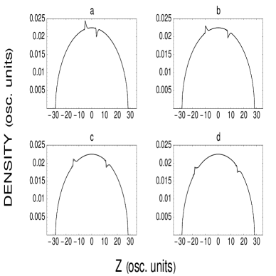
FIG. 1.: Density profiles of 1D noninteracting fermionic gas at different times: (a) 0.16, (b) 0.31, (c) 0.47, and (d) 0.63 in units of $1/\omega$ after imprinting a single phase step of $\phi_{0}=2.0\,\pi$ and $\zeta=0.5$ osc. units. Note that each graph consists actually of two curves: one obtained based on the many–body Schrödinger equation (solid line) and the second coming from the one–dimensional Thomas–Fermi model (dashed line).

It is important to verify the above scenario in more than one–dimensional space. To this end, let’s consider a noninteracting Fermi gas in an arbitrary three–dimensional harmonic trap characterized by the frequencies $\omega_{x}$, $\omega_{y}$, and $\omega_{z}$. One–particle orbitals are taken as a product $\,\varphi_{n_{x}}^{(1)}(x)\,\varphi_{n_{y}}^{(2)}(y)\,\varphi_{n_{z}}^{(3)}(z)$ of eigenvectors of the Hamiltonians of one–dimensional harmonic oscillators. The phase is being imprinted in the same form as in one–dimensional case. Since the Hamiltonian separates in coordinates ’x’, ’y’, and ’z’, the time propagation of each orbital after phase imprinting can be easily reduced to one–dimensional problem:

$$\Psi_{n_{x}n_{y}n_{z}}(x,y,z,t) = e^{-i\rm{E}_{n_{x}}t/\hbar}\>e^{-i\rm{E}_{n_{y}}t/\hbar}$$

$$\times \varphi_{n_{x}}^{(1)}(x,0)\,\varphi_{n_{y}}^{(2)}(y,0)$$

$$\times \varphi_{n_{z}}^{(3)}(z,t)$$

where

$$\varphi_{n_{z}}^{(3)}(z,t) = e^{-i\rm{H_{z}}\,t/\hbar}\varphi_{n_{z}}^{(3)}(z,0)\,e^{i\phi(z)}$$

and $\rm{H_{z}}$ is the Hamiltonian of one–dimensional harmonic oscillator. Now the diagonal part of one–particle density matrix is given by the expression:

$$\rho(\vec{r},t)=\frac{1}{\rm{N}}\,\sum_{\rm{E}_{n_{x}n_{y}n_{z}}\leq\rm{E}_{F}}\,|\varphi_{n_{x}}^{(1)}(x,0)|^{2}\;|\varphi_{n_{y}}^{(2)}(y,0)|^{2}$$ (1)

(2)

$$\times\,|\varphi_{n_{z}}^{(3)}(z,t)|^{2}\phantom{aaaaaaaaaa}\,$$ (3)

where $\rm{N}$ is the number of atoms and sum is performed over the one–particle states below Fermi energy.

One of the obvious regimes where the Thomas–Fermi approximation holds is that of a cigar–shaped trap elongated enough, depending on the number of confined atoms. For example, in the case of a ground state of N=$400$ fermions in the harmonic potential with oscillator frequencies taken as $\omega_{x}=\omega_{y}=400\omega_{z}$ only the smallest possible radial quantum numbers are involved: $n_{x}=n_{y}=0$. It follows from the formula (3) that the density along ’z’ axis (or any line parallel to it) is just one–dimensional density multiplied by a constant. Certainly, the overall behavior found in one–dimensional case translates to three-dimensional one. Conditions presented above could be considered also as a criterion for treating the real Fermi gas as a one–dimensional system.

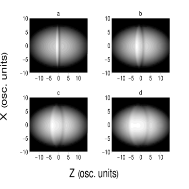
FIG. 2.: Images of the fermionic density of N=$1000$ atoms after writing a single phase step of $1.0\,\pi$ and $\zeta=0.2$ osc. units onto a three–dimensional noninteracting Fermi gas confined in a trap configured as follows: $\omega_{x}=2\,\omega_{z}$ and $\omega_{y}=64\,\omega_{z}$. The snapshots are taken at times of (a) 0.10, (b) 0.25, (c) 0.40, and (d) 0.60 in units of $1/\omega_{x}$ .

Now we start to depart from “one–dimensional” geometry. In Figs. 2 and 3 we show the contour plots of density in the ’xz’ plane and the density profiles along ’z’ direction respectively after writing a single phase step onto a three–dimensional gas, although confined in a disk–shaped trap. The system behaves effectively as a two–dimensional gas; the number of atoms and the fundamental frequencies are chosen in such a way that one ($n_{y}$) of the quantum numbers equals zero. In this case we again observe two pulses moving in opposite directions, however they are broader in comparison with one–dimensional case (see Figs. 1 and 3). At the same time results obtained based on the Thomas–Fermi approximation differ qualitatively, showing the existence of the second dark soliton. Only going to much larger number of atoms improves the agreement between both approaches, however then all structures are getting less pronounced. In three-dimensional spherically symmetric trap we have never observed double pulse behavior. Instead of that, the dark soliton and the density wave are generated (see Fig. 4) much as in the case of solitons generated in the Bose–Einstein condensate [8]. The dark soliton propagates with the velocity smaller than the speed of sound and experiences (as in one–dimensional case) the oscillatory motion.

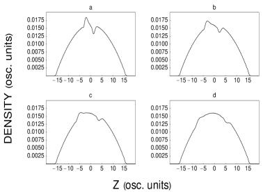
FIG. 3.: Evolution of the density distribution of $1000$ Fermi atoms in three–dimensional harmonic trap ( $\omega_{x}=2\,\omega_{z}$ and $\omega_{y}=64\,\omega_{z}$) after imprinting a single phase step of $\phi_{0}=1.0\,\pi$ and $\zeta=0.2$ osc. units. The successive frames correspond to moments: (a) 0.25, (b) 0.40, (c) 0.60, and (d) 0.85 in units of $1/\omega_{x}$.

A convenient way to discuss Thomas–Fermi approximation is to start from a set of equations for reduced density matrices. Since there is no interaction between particles, the equation of motion for the one–particle density matrix does not involve the two–particle density matrix $\rho_{2}$ and is given by [12]

$$i\hbar\frac{\partial}{\partial t}\rho_{1}(\vec{r}_{1},\vec{r}_{2},t)=-\frac{\hbar^{2}}{2m}(\vec{\nabla}_{1}^{2}-\vec{\nabla}_{2}^{2})\,\rho_{1}(\vec{r}_{1},\vec{r}_{2},t)\phantom{11111}$$ (4)

$$+\left[V_{ext}(\vec{r}_{1},t)-V_{ext}(\vec{r}_{2},t)\right]\rho_{1}(\vec{r}_{1},\vec{r}_{2},t)\;,\phantom{11111111111l}$$ (5)

where $V_{ext}(\vec{r},t)$ is the external potential. In the limit $\vec{r}_{1}\rightarrow\vec{r}_{2}$ Eq. (5) leads to the continuity equation

$$\frac{\partial\rho(\vec{r},t)}{\partial t}+\vec{\nabla}\cdot\left[\rho(\vec{r},t)\,\vec{v}(\vec{r},t)\right] = 0\;,$$ (6)

where the density and velocity fields are defined as follows:

$$\rho(\vec{r},t) = \lim_{\vec{r}_{1}\rightarrow\vec{r}_{2}}\rho_{1}(\vec{r}_{1},\vec{r}_{2},t)$$ (7)

$$\vec{v}(\vec{r},t) = \frac{\hbar}{2m}\lim_{\vec{r}_{1}\rightarrow\vec{r}_{2}}(\vec{\nabla}_{1}-\vec{\nabla}_{2})\,\chi_{1}(\vec{r}_{1},\vec{r}_{2},t)$$ (8)

and $\chi_{1}(\vec{r}_{1},\vec{r}_{2},t)$ is the phase of the one–particle density matrix.

One can also rewrite Eq. (5) introducing the center–of–mass ($\vec{R}=(\vec{r}_{1}+\vec{r}_{2})/2$) and the relative position ($\vec{s}=\vec{r}_{1}-\vec{r}_{2}$) coordinates. By taking the derivative of Eq. (5) with respect to the coordinate $\vec{s}$ the hydrodynamic Euler–type equation of motion is obtained in the limit $\vec{s}\rightarrow 0$

$$\frac{\partial\vec{v}(\vec{r},t)}{\partial t} = -\frac{\vec{\nabla}\cdot T}{m\,\rho(\vec{r},t)}-\frac{1}{2}\vec{\nabla}\vec{v}^{\,2}(\vec{r},t)-\frac{\vec{\nabla}V_{ext}(\vec{r},t)}{m}\;.$$ (9)

Here, the kinetic–energy stress tensor $T$, whose elements are given by

$$T_{kl} = -\frac{\hbar^{2}}{m}\lim_{\vec{s}\rightarrow 0}\frac{\partial^{\,2}\sigma_{1}(\vec{R},\vec{s},t)}{\partial s_{k}\partial s_{l}}\;,$$

depends on the one–particle density matrix (more precisely on its amplitude $\sigma_{1}(\vec{r}_{1},\vec{r}_{2},t)$) and is calculated based on a local equilibrium assumption which is the substance of Thomas–Fermi approximation.

FIG. 4.: Evolution of the density distribution of $10^{4}$ Fermi atoms in three–dimensional spherically symmetric harmonic trap after writing a single phase step of $2.0\,\pi$ and $\zeta=0.5$ osc. units. The successive frames correspond to moments: (a) 0.1, (b) 0.2, (c) 0.3, and (d) 0.4 in units of $1/\omega$.

We have solved the set of Eqs. (6) and (9) with kinetic–energy stress tensor approximated by its Thomas–Fermi form, i.e., diagonal tensor with (in three–dimensional case) $(\hbar^{2}/m)(1/30/\pi^{2})(6\pi^{2}\rho)^{5/3}$ term at each position. In fact, we applied the inverse Madelung transformation [13] to Eqs. (6) and (9) and used the Split-Operator method combined with the imaginary–time propagation technique (for generation of the ground state of the trapped Fermi gas) as well as the real–time propagation (for phase imprinting and analysis of dynamic instabilities after that).

By using the definition (8) of the velocity field one can easily calculate

$$\vec{v}(\vec{r},t) = \frac{\sum_{i=1}^{\rm{N}}\,\rho_{i}(\vec{r},t)\,\vec{v}_{i}(\vec{r},t)}{\sum_{i=1}^{\rm{N}}\,\rho_{i}(\vec{r},t)}\,.$$

Although the one–particle velocities $\vec{v}_{i}$ are irrotational, the global velocity is, in principle, rotational. Therefore, for an ultracold Fermi gas in a normal phase one should not expect the existence of quantized vortices. However, as we’ll see, the excitations of fermionic gas with a hole in a density along some line (or a dot in two–dimensional case) and non–zero circulation around this line are still possible.

To discuss the possibility of generation of vortices in a degenerate Fermi gas we involve the polar coordinates. Hence, the eigenvectors are given by: $\Psi_{nm}(r,\phi)=A\,r^{|m|}\>L_{n}^{|m|}(r^{2})\>e^{r^{2}/2}\,e^{im\phi}$ and $A^{2}=n!/[\pi(n+|m|)!]$. As in Refs. [14, 15], we pass a laser pulse through the appropriately tailored absorption plate before impinging it on the atomic gas. The laser pulse is short with a duration of the order of the fraction of microsecond and the frequency is detuned far from the atomic transition (only the dipole force is important). Under such conditions the atomic motion is negligible during the pulse and the only effect of light on the atoms is imprinting the phase. To generate a vortex one has to prepare the absorption plate with azimuthally varying absorption coefficient. Changing the laser intensity and the duration of a pulse (the laser pulse area) one is able to design various vortex excitations of the Fermi gas. The state right after phase imprinting turns out to be dynamically unstable and soon after a vortex at the center of the trap is formed. In Fig. 5 we show the density after the pulse with the laser pulse area equal to $3\times 2\pi$ was applied to the system of N=$6$ fermions. The stable, not quantized vortex is generated. Increasing the number of atoms leads to the lower contrast of the vortex but increasing (keeping the same number of atoms) the pulse area restores the contrast.

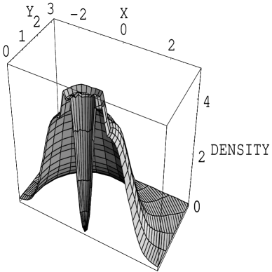
FIG. 5.: Density (in arbitrary units) of the system of N=$6$ fermions in the excited state with a vortex.

In conclusion, we have shown that the phase imprinting method can be employed for generation of solitons and vortices in ultracold fermionic gases. We have demonstrated that idea explicitly by solving the many–body Schrödinger equation for a gas of noninteracting neutral fermionic atoms. There exists differences in comparison with the Bose–Einstein condensate case. For example, the presence of bright solitons moving with the velocity higher than the speed of sound or the nature of the vortices which are not quantized. All these phenomena present for fermionic gases have nothing to do with the potential formation of bound states (Cooper pairs) followed by the condensation, since no interaction between Fermi atoms was included in the calculations.

REFERENCES

- [1] B. DeMarco and D.S. Jin, Science 285, 1703 (1999).
- [2] G.M. Bruun and C.W. Clark, Phys. Rev. Lett. 83, 5415 (1999).
- [3] G.M. Bruun and K. Burnett, Phys. Rev. A 58, 2427 (1998).
- [4] K. Góral, B.-G. Englert, and K. Rza̧żewski, Phys. Rev. A 63, 033606 (2001).
- [5] M.A. Baranov and D.S. Petrov, Phys. Rev. A 58, R801 (1998); G. Bruun, Y. Castin, R. Dum, and K. Burnett, Eur. Phys. J. D 7, 433 (1999); P. Törmä and P. Zoller, Phys. Rev. Lett. 85, 487 (2000).
- [6] M.R. Matthews et al., Phys. Rev. Lett. 83, 2498 (1999).
- [7] K.W. Madison et al., Phys. Rev. Lett. 84, 806 (2000).
- [8] S. Burger et al., Phys. Rev. Lett. 83, 5198 (1999).
- [9] J. Denschlag et al., Science 287, 97 (2000).
- [10] Th. Busch and J.R. Anglin, Phys. Rev. Lett. 84, 2298 (2000).
- [11] M.D. Girardeau and E.M. Wright, Phys. Rev. Lett. 84, 5691 (2000).
- [12] H. Frölich, Physica 37, 215 (1967).
- [13] B.Kr. Dey and B.M. Deb, Int. J. Quantum Chem. 70, 441 (1998); A. Domps, P.-G. Reinhard, and E. Suraud, Phys. Rev. Lett. 80, 5520 (1998).
- [14] Ł. Dobrek et al., Phys. Rev. A 60, R3381 (1999).
- [15] G. Andrelczyk et al., Phys. Rev. A 64, 043601 (2001).