Measurements of Particle Dynamics in Slow, Dense Granular Couette Flow

Abstract

Experimental measurements of particle dynamics on the lower surface of a 3D Couette cell containing monodisperse spheres are reported. The average radial density and velocity profiles are similar to those previously measured within the bulk and on the lower surface of the 3D cell filled with mustard seeds. Observations of the evolution of particle velocities over time reveal distinct motion events, intervals where previously stationary particles move for a short duration before jamming again. The cross-correlation between the velocities of two particles at a given distance $r$ from the moving wall reveals a characteristic lengthscale over which the particles are correlated. The autocorrelation of a single particle’s velocity reveals a characteristic timescale $\tau$ which decreases with distance from the inner moving wall. This may be attributed to the increasing rarity at which the discrete motion events occur and the reduced duration of those events at large $r$. The relationship between the RMS azimuthal velocity fluctuations, $\delta v_{\theta}(r)$, and average shear rate, $\dot{\gamma}(r)$, was found to be $\delta v_{\theta}\propto\dot{\gamma}^{\alpha}$ with $\alpha=0.52\pm 0.04$. These observations are compared with other recent experiments and with the modified hydrodynamic model recently introduced by Bocquet et al.

Introduction

The detailed understanding of slow flow in dense granular systems has remained one of the central challenges in the field of granular materials [1]. While fast dilute granular flows are fluid-like and can be described well by granular kinetic theory [2, 3, 4], slow flows at high packing fraction preserve many of the complex properties of static granular packs and may be more accurately described as slow, plastic deformation of a metastable granular solid than flow of a fluid. Recent work by Howell and Behringer [5, 6] showed that many of the intriguing properties of granular solids, such as the broad distribution of stresses and the presence of “force chains” which focus stresses along paths of many connected particles, play a crucial role. Direct visualization revealed that the flow is intermittant in time and that correlations, both in time and in space, exist [7]. These are seen as intervals over which one or more particles in a region become unjammed, move for a short time, and then become jammed again. Such properties of dense granular flow are reminiscent of behavior seen in glasses, dense colloidal suspensions, and foams [8]. Recent studies have been successful at relating stresses in stationary bead packs with those in glassy fluids [9], suggesting the two systems may also have similar flow properties for high packing fractions and low shearing rates. It is hoped that an understanding of dense granular flow will provide insight into the properties of static granular packs as well as the broader class of jammed systems.

From previous work a number of unresolved fundamental questions about slow, dense granular shear flow emerge. Although videos and plots of particle trajectories suggest that particle velocities are correlated both in space and in time, these correlations have not been directly measured or characterized, and their effect on the overall flow behavior is unknown. Previous experiments performed with various granular materials [10, 11] have shown that the microscopic properties of a material such as particle shape, polydispersity, and surface friction manifest themselves in the macroscopic flow behavior; however the details of how the microscopic particle properties and dynamics influence the overall flow is not fully understood. A number of theories describe the flow by relying on coarse-grained quantities, such as an effective temperature or viscosity. However, as we show here, rather than vary smoothly and monotonically, these quantities change abruptly and even oscillate on sub-particle lengthscales which may make it difficult to capture the full behavior in a coarse-grained model. The lack of a complete experimental description of the system, especially on the microscopic scale, has so far prevented the rigorous testing of any of these models.

To resolve these issues, a detailed description of the particle dynamics on the microscopic, ie. single particle level, is needed. While a number of careful, high-resolution, measurements [6, 10, 12, 13, 14, 15, 16] of the average macroscopic properties of slow, dense Couette flow have been performed, a detailed description of the microscopic dynamics has been lacking. The goal of the experiments reported in this article is to characterize the particle dynamics on both microscopic and mesoscopic scales, and to measure both the average properties of the material as well as the fluctuations about the mean.

To this end a systematic study of the dynamics of particles on the lower surface of a three-dimensional (3D) Couette cell was performed. The dynamics were captured with digital video, and individual particles were tracked through time. Accurate measurements of the particle velocity fluctuations and correlations required high-precision measurements of the particle positions in every video frame. In contrast to measurements of the time-averaged velocity or density profile, where the effects of measurement noise is reduced by sufficient averaging [10], high-bandwidth fluctuation measurements are limited by the precision of each position measurement. For this reason, a number of improvements in the position measurement technique were implemented and extensive calibration experiments made it possible to mitigate the effects of instrumental noise on the fluctuation and correlation measurements.

With these improvements, I was able to measure correlations in particle velocities and to obtain the correlation length $\xi$ and correlation time $\tau$. The improved resolution also allowed me to measure the distribution and amplitude of the velocity fluctuations over a much larger range than was previously possible. The ability to determine, locally and simultaneously in the same system the packing fraction, average velocity, and fluctuation amplitude allowed for a direct comparison with granular kinetic or hydrodynamic models, such as the recent model by Bocquet et al. [16].

Background

Recently, several experiments on slow granular flows have been performed in the Couette geometry, both in two-dimensional (2D) [13, 6] and 3D [12, 10, 14, 15, 16] systems. The Couette geometry (see Fig. 1A) with uniformly rotating inner cylinder provides a steady-state flow which can be maintained for very long times and has a symmetry for azimuthal averaging of many quantities of interest. The break-up of the system into a shear band near the inner cylinder and an essentially stagnant material near the outer cylinder furthermore provides a single system in which velocities vary substantially through the cell allowing one to view faster and slower shearing regions simultaneously.

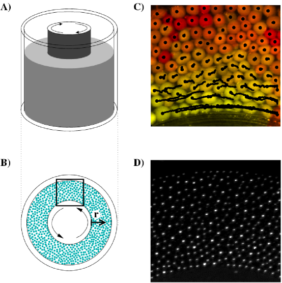
FIG. 1.: Sketch of the Couette cell and images of the lower surface. (A) The Couette cell consists of two coaxial cylinders of radii 25.0 and 41.5 mm. The gap between the cylinders is filled with a granular material and the inner cylinder is rotated at constant angular velocity. (B) The motion of the particles near the lower surface is recorded with a high speed digital camera at 250 frames per second. The region imaged is represented by the rectangle. (C) The trajectory and average velocity of each particle over the previous 200 ms (indicated by the particle shade: brighter for fast or darker for slow) are shown for mustard seeds, obtained using particle tracking techniques. (D) An example image of the cell filled with stainless steel bearing balls which are used for experiments requiring high precision position measurements.

Because dry granular materials are opaque, observations are either confined to 2D Couette cells [13, 6] and to the outer surfaces of 3D cells [10, 14, 15, 16], where optical tracking of surface particles is possible, or non-invasive 3D imaging tools must be employed [12, 10]. For 2D systems and the surfaces of 3D systems, the motion is typically recorded with video and each particle’s motion is tracked in the digitized frames using software. This approach has the benefit of providing detailed information about the particle dynamics. However, it is unable to probe the bulk behavior of a 3D system. Furthermore, packing fractions can only be determined where the particles are guaranteed to lie in the imaging plane, such as along the lower surface of the container. Non-invasive 3D imaging techniques, such as MRI and X-ray tomography, can be very effective at measuring certain properties of a 3D system. X-ray tomography is very well suited for measuring the time-averaged packing fraction [10] and is a valuable imaging tool [10, 17, 18]. However, determining the precise particle positions in 3D is computationally expensive and data acquisition rates are very slow, making 3D particle tracking studies difficult. MRI has proven itself as a powerful tool for measuring the time-averaged velocity inside 3D granular flows [19, 20, 21] and has been used to measure the average flow properties within the bulk in granular Couette flow [10]. MRI has also been used to measure the diffusion coefficient and correlation times for flowing granular material [22, 23].

Several groups have studied the time-averaged steady-state flow velocity in slow, dense granular Couette flow in both 2D and 3D  [12, 13, 6, 15, 10, 14, 16]. Typically one measures the average particle velocity in the azimuthal ($\hat{\theta}$) direction, $v_{\theta}(r)$, as a function of the distance $r$ from the moving inner cylinder wall. These studies reveal that the velocity decays quickly with $r$, with most shear occurring in a relatively narrow shear band of about 10 grains across for a broad range of parameters. High precision MRI measurements in 3D [10] have shown that $v_{\theta}(r)$ can be expressed as a product of an exponential decay and a Gaussian:

$$v_{\theta}(r)=v_{0}{\rm exp}[-{\rm b}(r/{\rm d})]{\rm exp}[-{\rm c}(({r-r_{0})/{\rm d}})^{2}].$$ (1)

The exponential term was found to be associated with the formation of layers (see Fig. 2D, adapted from [10]) which can slip past each other for systems of smooth, monodisperse spheres. For these materials, the exponential term dominates (see Fig. 2B) in both 3D [10, 14] and 2D [13, 6] systems. Note that, although the exponential term dominates for these systems, the Gaussian term is still present and gives rise to a characteristic, downward concave curvature on a log-linear plot (inset to Fig. 2B). For systems of particles which are aspherical, polydisperse, or rough, the exponential term essentially vanishes and a pure Gaussian velocity profile is observed in 3D [10](Fig. 2A). The center of the Gaussian was found to be at the inner cylinder wall (ie. $r_{0}\approx 0$), as seen in the inset to Fig. 2A. Thus, Eq. 1 can be recast into:

$$v_{\theta}(r)=v_{0}{\rm exp}[-(r/\lambda)-(r/\sigma)^{2}].$$ (2)

where the fitting parameters $\lambda$ and $\sigma$ describe the decay lengths of the exponential and Gaussian components, respectively. Note that unlike a pure exponential profile, in which $r$ can be translated to a new origin with a simple rescaling of the velocity, the Gaussian component has a center position, $r_{0}\approx 0$, which specifies a unique reference location in the system.

FIG. 2.: The velocity and density profiles in the bulk for poppy and mustard seeds adapted from [10]. The radial profile of the azimuthal velocity $v_{\theta}(r)$ within the bulk of a 3D sample of poppy seeds (A) and mustard seeds(B) was previously measured using MRI. The inner layer of particles of diameter ${\rm d}$, between $r/{\rm d}=0$ and $r/{\rm d}=1$, was glued to the inner cylinder wall and thus exhibits a nearly constant velocity profile, while the free material for $r/{\rm d}>1$ experiences shear flow. The velocity profile for poppy seeds (${\rm d}=0.8{\rm mm}$) was found to be Gaussian in shape and rate independent (inset to A). The velocity profile for mustard seeds (${\rm d}=1.8{\rm mm}$) exhibits sharp drops and steps because MRI measures the mass flow velocity which differs from the velocity profile for particle centers if significant layering of particles occurs. The velocity profile $v_{\theta}(r)$ for mustard seeds in the middle of the cell as determined by MRI was compared to that on the bottom surface of the cell, as measured by particle tracking in videos (inset to B). The comparison reveals that the flow within the bulk and on the lower surface have the same overall shape. The density profile inside the 3D system was measured using X-ray tomography for samples of poppy seeds (C) and mustard seeds (D). While little ordering is observable for poppy seeds, pronounced oscillations in $\rho(r)$ for mustard seeds reveals that the particles are layering along the moving inner cylinder wall.

In the slow shearing regime, the velocity profile normalized by the shear rate was found to be invariant to the imposed shear rate at the inner wall [6, 10, 14]. Furthermore, using MRI in 3D the velocity profile $v_{\theta}(r)$ was found [10] to be uniform throughout the height of the cell to within several particles (the detectable limit) of the upper and lower surfaces. Comparison of MRI measurements with video data obtained from the lower cell surface revealed [10] that the bottom layer of particles has the same average velocity profile as the interior (see inset to Fig. 2B). This is likely caused by the relative smoothness of the lower boundary surface, contrasted with the geometrically rough surface of the bulk granular material above the lowest layer of particles. Particles on the lower surface are moved with the bulk material above it since these forces dominate the relatively small frictional forces on the lower surface. A direct comparison of the upper free surface with the bulk was not performed because significant heaping (several particle diameters) occurred at the top surface making video tracking of these particles difficult.

Granular Couette flow experiments in 2D and 3D vary in several important ways. In 2D, the Couette cell imposes a constant volume and thus fixed average packing fraction on the system as a whole. Since no dilation into the vertical direction (against gravity) can occur, this leads to a strong dependence of the flow properties on the average packing fraction [13, 6]. In a 3D Couette cell with free top surface, the packing fraction can adjust freely in response to gravity, Reynolds dilation, and vibratory compaction until a local steady-state packing fraction is reached. Thus, the steady-state behavior of the 3D system does not exhibit the transitions in behavior observed in 2D systems when the initial packing fraction is varied. While both 2D and 3D systems give similar velocity profiles $v_{\theta}(r)$ for nearly monodisperse, smooth spheres, they are found to differ qualitatively for irregularly shaped particles as experiments in 2D have found a nearly pure exponential form [24]. It has been speculated that this may be caused by differences in the dimensionality of clusters of correlated particles [25] or possibly by differences in the way particles rotate (spin) in the two systems [11].

Qualitative properties of the flow can be determined from videos or from graphs showing the trajectories of particles through time, such as the one shown in Fig. 1C, revealing that the motion is intermittent in time. These imaging tools also give first hints that particles are correlated in space: Clusters of particles can be seen to move together for short intervals. By watching the motion of particles which are far from the moving wall, one is able to observe motion events which involve the collective rearrangement of many particles in the system, from the inner wall out to larger $r$. This suggests that buckling of force chains, radiating outward from the moving wall, causes failure events that result in particle rearrangements. Experiments performed in 2D with birefringent disks have been able to visualize these force chains and their dynamic evolution directly [6].

Recent studies by the Haverford/Penn group of the top surface of 3D Couette flow [14, 16] show that the average flow on the top surface resembles, at least qualitatively, that observed in other parts of 3D systems: the velocity profile $v_{\theta}(r)$ is between exponential and Gaussian in shape, and for polydisperse materials $v_{\theta}(r)$ decays more slowly and is more Gaussian than for monodisperse materials [26]. These experiments also measured the RMS velocity fluctuations, $\delta v_{\theta}(r)$ and $\delta v_{r}(r)$, in the azimuthal and radial directions and found that these fluctuations decayed more slowly with $r$ than does the average velocity, $v_{\theta}(r)$. In addition, the shear rate, $\dot{\gamma}\equiv\partial v_{\theta}/\partial r$, was observed to scale with the fluctuations as $\delta v_{\theta}(r)\propto\dot{\gamma}^{\alpha}$, where $\alpha=0.4$.

The upper surface of 3D Couette flow was also studied by the Caltech group [15]. They observed a measurable secondary flow which moved from the outer cylinder to the inner cylinder, and down the inner cylinder wall, giving rise to heaping on the upper surface. These experiments confirmed the rate-independence of the azimuthal flow although no functional form for $v_{\theta}(r)$ was given. The RMS velocity fluctuations about their mean, $\delta v_{\theta}(r)$ and $\delta v_{r}(r)$, were also measured.

Several theories have been put forth to describe granular flow. The most well-studied of these is granular kinetic theory [4], which locally relates the stress to the fluctuations and energy dissipation using coarse-grained variables. This theory assumes that collisions are instantaneous and binary, which typically requires the flow velocity to be large and particle density to be low. In this limit, the flow is not expected to be shear rate independent and $\delta v\sim\dot{\gamma}$ [27]. In the slow, dense flow limit, on the other hand, particles often have multiple, persistent contacts and forces are transmitted along dynamically rearranging force chains. Recently, Bocquet et al. have proposed [16] an extension of kinetic theory for the dense flow regime. This continuum model makes some of the same key assumptions as kinetic theory, but tries to capture the behavior in the dense limit by proposing a stronger divergence of the viscosity with packing fraction as the random close packed limit is approached. This leads to $\delta v\sim\dot{\gamma}^{\alpha}$ with $\alpha<1$.

A number of discrete models have been proposed which attempt to capture the intermittancy and correlation in particle motion seen in videos of the particle flow and expected for a well-connected system similar to the static bead packs. Debregeas and Josserand [25] suggest the material flows in clusters of various sizes on short timescales and predict that the average flow profile, $v_{\theta}(r)$, should be Gaussian in 3D and exponential in 2D. This is consistent with existing data on irregularly-shaped particles in 2D [24] and 3D systems [10], although not for monodisperse, round particles where layers form and slip past each other. A second approach proposed by Josserand [28], which also predicts profiles for $v_{\theta}(r)$ which vary from exponential to Gaussian, is based on a lattice model which directly correlates particle motion from one layer to the next. Here the coupling between particles, possibly related to surface and geometrical friction, is the control parameter which determines the form of $v_{\theta}(r)$. Tkachenko and Putkaradze [29] model correlated cluster motion in yet another way, arriving at a form for $v_{\theta}(r)$ which varies from a Gaussian to exponential depending on the packing fraction profile to which the system relaxes. Each of these models, based on different physical assumptions, attempts to capture the cooperative rearrangements observed in videos of the shear flow.

Experimental Method

The experimental apparatus used for the studies described in this article was the same, with only minor modifications, as that used in previous studies [10] which measured the radial profile of the steady-state azimuthal flow, $v_{\theta}(r)$, at various heights using MRI. The granular material was confined between two coaxial cylinders of diameters 51 mm and 82 mm (see Fig. 1A). The outer cylinder and cell floor were held stationary while the inner cylinder was rotated at constant velocity (the velocity of the inner wall was $v_{\rm wall}\approx 23{\rm mm/s}$ for all experiments described in this article). To provide a reproducible source of friction, each cylinder surface had a layer of particles glued to it. A portion of the lower surface of the cell was imaged (see Fig. 1B) at 250 fps and 256x240 pixel resolution using a monochrome Kodak Motion Corder Analyzer digital camera.

Our previous particle tracking experiments using seeds or glass spheres showed that the motion was intermittent and correlated in space (see Fig. 1C), and that the time-averaged azimuthal flow profile, $v_{\theta}(r)$, on the lower surface was similar to that at other heights within the cell. However, these experiments were unable to measure directly the fluctuations in the particle velocities or the correlations between particle velocities due to insufficient resolution in determining the exact trajectories of each particle.

In order to obtain the necessary resolution in measuring the particle trajectories, a number of modifications were made. The most important of these changes was to use polished stainless steel balls (manufactured for ball bearings). Illuminating the cell with a single small light source produced a small, well-defined reflection from each particle (see Fig. 1D) which allowed for a very precise position measurement. The high degree of sphericity of ball bearing balls ($\delta r/r\leq 10^{-4}$ for the grade 100 balls used) almost completely eliminated the false motion of particles observed when less precise spheres, such as commonly available glass spheres [30], were used. It was also essential to minimize blemishes in the lower surface which may introduce noise into particle position measurements. To maximize the spatial resolution of each position measurement, I spread out the light reflected from each particle across as many pixels as possible. This was done by defocussing the lens, producing a small annulus for each particle [31, 32]. I determined the uncertainty $\delta_{x}$ in each position measurement from all noise contributions by performing test runs with a system in which all particles were glued to a disk. At very slow disc rotation rates, the noise in position measurement was 0.05 pixels or 4 $\mu{\rm m}$. By analyzing video data of completely stationary particles, I found the same fluctuation in measured position, indicating that this noise floor in the position measurement was introduced by pixel noise in the camera. This was confirmed by directly measuring the pixel noise in the camera and calculating the uncertainty this introduced into the center of mass measurement.

To eliminate crystallization, which occurs very rapidly for highly monodisperse spheres against a flat surface, a bidisperse sample was used. The sample consisted of 1.0 and 1.5 mm balls mixed in equal quantities by weight. Along the bottom surface and in the primary shear zone near the moving wall, the larger particles were observed to gradually move away from the lower surface. This presumably occurs because the contact angle between smaller and larger spheres on the lower surface has a non-zero angle relative to that surface, giving rise to a vertical component in any contact force. This pushes larger particles out of the bottom layer of particles. However, the small concentration of larger balls which remained on the lower surface, primarily at larger distances from the moving wall, was sufficient to prevent crystalline ordering [33]. As will be discussed further below, aside from the lack of crystalline ordering the system behaved as if it were monodisperse.

Each experimental run consisted of 5459 digital video frames of resolution 256x240 pixels and imaging approximately 350 particles. The position of each particle in each frame was measured using a convolution method which determined the center of brightness of each reflection [34]. From these sets of positions at each time, the particle trajectories were assembled and the velocities were determined. Each experimental run yielded approximately 2,000,000 velocity measurements. Typically, between three and five runs of each experimental type were performed. These were either averaged or compared to guarantee reproducibility of the results.

The average velocity and density profiles and the velocity correlations were affected very little by random noise. However, velocity fluctuation measurements do not distinguish between actual fluctuations in the particle motion and noise in the particle position measurements. This noise is caused by various effects including camera pixel noise, optical artifacts, pixelation, assumptions in software, and imperfections in the spheres. To determine the net contribution of this measurement noise to the fluctuation measurements, calibration experiments were performed. The calibration was done by fixing particles to a disk which was moved at constant angular velocity. Although the particles move along uniform arcs, the measured trajectories have a non-negligible noise level which varies with disk rotation rate. A wide range of rotation rates was used to obtain calibrations for use at various locations in the cell, since the average particle velocity varies through the cell. These calibration experiments were analyzed in exactly the same way as the other experiments. Using these calibrations, the fluctuation measurements were corrected, extending the range over which the velocity fluctuations could be reliably measured significantly.

Experimental Results

Average velocity and density profiles

The radial profile of the time-averaged azimuthal velocity, $v_{\theta}(r)$, was obtained by averaging the velocities of all particles over all times at each radius $r$ (see Fig. 3A). I found that $v_{\theta}(r)$ was well-fit by Eq. 2 with $\lambda=(2.1\pm 0.2){\rm d}$ and $\sigma=(4.7\pm 0.4){\rm d}$ (solid line in Fig. 3A and inset). This profile has a dominant exponential term, similar to measurements of nearly monodisperse samples of smooth spheres [10]. The velocity profile is smooth and does not show the strong steps seen with MRI experiments, as video techniques track the particle center motion and not the average flow of material, as MRI does. For materials for which the packing fraction profile, $\rho(r)$, oscillates significantly, such as smooth monodisperse spheres, the mass flow profile measured by MRI exhibits steps in the velocity profile (as seen in Fig. 2B). Note also that, for $r<1$, the mean flow velocity profile is essentially constant as these particles are glued to the moving inner cell wall.

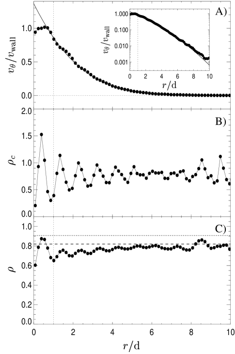
FIG. 3.: Radial velocity and density profiles. The material between $r/{\rm d}=0$ and $r/{\rm d}=1$ is glued to the inner wall giving rise to a nearly constant velocity profile. (A) The velocity profile for essentially monodisperse bearing balls (${\rm d}=1.0{\rm mm}$), fit to Eq. 2. The dashed line at $r/d=1$ represents the edge of the layer of particles glued to the inner cell wall. When plotted semi-log (inset), $v(r)$ is seen to be dominated by the exponential term with very weak curvature, as expected for a nearly monodisperse sample of smooth spheres. (B) The distribution of particle centers, $\rho_{c}(r)$, showing pronounced layering. (C) The local packing fraction of material, $\rho(r)$, calculated from $\rho_{c}(r)$. The horizontal dotted line represents the density of a crystal in 2D, $\rho_{\rm xtal}^{\rm 2D}=0.91$, and the horizontal dashed line represents that of random close packed spheres in 2D, $\rho_{\rm rcp}^{\rm 2D}=0.82$.

The radial distribution of particle center positions can be used to calculate the particle center packing fraction $\rho_{c}(r)$ (Fig 3B) which is normalized such that $\rho_{c}(r)=1$ would correspond to all space being occupied by material. Pronounced oscillations are visible in $\rho_{c}(r)$ corresponding to ordering of the particles into concentric layers. This layering is generally only observed for smooth spherical particles and accompanies the predominantly exponential form of $v_{\theta}(r)$ [10].

By convolving $\rho_{c}(r)$ with a kernel describing the cross-sectional area of an individual particle, one obtains the material packing fraction $\rho(r)$ (see Fig. 3C). Because the video images show the number of particles over a given area, the kernel used is the cross-section of a disk and both $\rho_{c}(r)$ and $\rho(r)$ are 2D quantities. In order to calculate the packing fraction accurately, the local relative populations of smaller and larger spheres at each radius $r$ in the cell were measured and used when calculating $\rho(r)$. The layering of particles is still observable in $\rho(r)$ although it is much more subtle than in $\rho_{c}(r)$. Reynolds dilation is also visible at small $r$. At larger $r$, $\rho(r)$ approaches the random close packing fraction in 2D [35], $\rho_{\rm rcp}^{\rm 2D}=0.82$. (At the largest $r$, layering occurs again due to volume exclusion effect near the outer wall.)

Velocity-time traces

A first step toward quantifying the intermittant character of the flow is to plot the velocity of a single particle over time for randomly chosen particles at various positions in the cell. Several of these velocity traces are shown in Fig. 4. The left column shows the velocities of four different particles at different distances $r$ from the inner wall. The right column shows calibration data obtained by rotating a disk with particles glued to it at rates roughly giving the same average velocity as in the corresponding plot in the left column. The calibration data in the right column thus provides an indication of the velocity-dependent noise level, observable as the fluctuations in the signal $v(t)$.

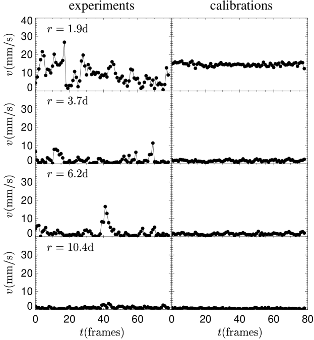
FIG. 4.: Time traces of the velocity of individual bearing balls at different radii. The velocity evolution over time (1 frame is 4 ms) for four randomly selected particles at radii 1.9d, 3.7d, 6.2d and 10.4d for an experimental run are shown in the left column. The right column shows calibration data obtained by tracking particles which were glued to a disk and rotated at velocities corresponding to the approximate average velocity for each particle in the experiment (left column). The amplitude of the fluctuations in the right column show the noise level for the given rotation rate. Distinct “motion events”, intervals over which a particle experiences significant motion, are clearly observable in the experimental runs. The frequency of the motion events is seen to decrease quickly with distance from the moving inner wall (at $r=10{\rm d}$ essentially no events occur during the 80-frame time interval), although the amplitude and duration only show a small decrease.

The velocity traces for experimental runs (left column) show distinct motion events during which appreciable particle motion persists. The duration of these events is typically several frames (one frame corresponds to 4 ms), and is roughly independent of radial position in the system. While some velocity changes are gradual over several frames, many large rapid increases and decreases in velocity are visible. These presumably correspond to very fast jamming and unjamming events. Although their amplitude does not vary strongly with $r$, the frequency of these events varies substantially, occurring at increasingly longer intervals for larger $r$.

Velocity distributions

The velocity components in the radial direction, $v_{r}$, and azimuthal direction, $v_{\theta}$, were histogrammed for all particles and times for several ranges of radii $r$ (Fig. 5). These velocities represent the measured average velocity between two successive video frames (ie. over 4 ms). The histogram of radial velocities $P(v_{r})$ is peaked at $v_{r}=0$ and is approximately symmetric about this point since the primary flow is not in the radial direction. The width of the distributions decrease with increasing distance $r$ from the rotating cell wall. The off-center distributions $P(v_{\theta})$ in (B) reflect the average azimuthal velocity, $v_{\theta}(r)$, as seen in Fig. 3A.

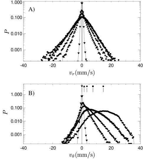
FIG. 5.: Distribution of particle velocity components. Histograms of the radial (A) and azimuthal (B) particle velocity components determined from two successive video frames (ie. averaged over 4 ms) are shown. Each curve represent particles at different radii: $r=1.5{\rm d}$ (circles), $r=2.5{\rm d}$ (squares), $r=3.6{\rm d}$ (diamonds), $r=4.6{\rm d}$ (triangles), $r=9.7{\rm d}$ (down-triangles). The average velocity in the azimuthal direction is plotted as small vertical lines at the top of the lower plot, labeled by the symbol of the curve which it corresponds to.

The average value of $v_{\theta}$ at each radius is shown by the position of the corresponding data point at the top of the graph. The velocity distributions $P(v_{\theta})$ are peaked near, but slightly below, their average value because there are larger velocity fluctuations in the forward direction. Fluctuations away from the mean velocity decay roughly exponentially, especially far from the inner cell wall, but acquire a rounded shape for small $r$.

Fluctuation amplitudes

The RMS velocity fluctuations in the radial and azimuthal directions were calculated using the set of all particle velocities collected over all times. The velocity fluctuation of the $i$’th particle about the mean at time $t$ is given by $\overrightarrow{\Delta v_{i,t}}\equiv\overrightarrow{v_{i,t}}-\overrightarrow{\bar{v}(r=r_{i,t})}$, where $\overrightarrow{v_{i,t}}$ is the velocity vector of the $i$’th particle at time $t$, $r_{i,t}$ is the distance of the $i$’th particle from the inner wall at time $t$, and $\overrightarrow{\bar{v}(r)}$ is the average velocity of all particles at distance $r$ from the inner wall. The RMS velocity fluctuations about the mean in the radial and azimuthal directions, $\delta v_{r}(r)$ and $\delta v_{\theta}(r)$, are given by

$$\delta v_{r}(r)=\sqrt{{\sum{\Delta{v_{r}}^{2}_{i,t}}\delta(r_{i,t}-r)}\over{\sum\delta(r_{i,t}-r)}},\delta v_{\theta}(r)=\sqrt{{\sum{\Delta{v_{\theta}}^{2}_{i,t}}\delta(r_{i,t}-r)}\over{\sum\delta(r_{i,t}-r)}}$$ (3)

where the sums are taken over all particles $i$ and times $t$, and $\Delta{v_{\theta}}$ and $\Delta v_{r}$ are the azimuthal and radial components of $\overrightarrow{\Delta v}$. The RMS fluctuation amplitudes $\delta v_{r}(r)$ (open squares) and $\delta v_{\theta}(r)$ (open circles) are shown in Fig. 6, along with the average azimuthal flow $v_{\theta}(r)$ (solid circles). The average fluctuation amplitude is seen to be somewhat smaller than $v_{\theta}(r)$ in the primary shear zone, but quickly dominates the azimuthal flow for $r>3$.

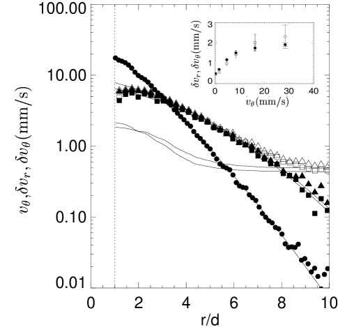
FIG. 6.: Velocity and velocity fluctuation profiles. The velocity profile (solid circles) is shown with its fit to Eq. 2. The azimuthal and radial RMS velocity fluctuations about their mean, $\delta v_{r}(r)$ (open squares) and $\delta v_{\theta}(r)$ (open circles) as defined in Eq. 3 are also shown. The inset shows the background values of $\delta v_{r}(r)$ and $\delta v_{\theta}(r)$ measured from calibrations performed by glueing particles to a disk which was rotated at various speeds. Using this calibration and the average velocity profile $v_{\theta}(r)$ (solid circles), the noise floors for $\delta v_{r}(r)$ and $\delta v_{\theta}(r)$ were determined (two lower solid curves). The corrected curves for $\delta v_{r}(r)$ and $\delta v_{\theta}(r)$ (solid circles and triangles) were obtained by subtracting the contribution from the noise floors [36]. The corrected fluctuation profiles are shown with fits to Eq. 4.

By measuring the RMS fluctuation amplitude in calibration experiments taken at varying rotation rates (see inset to Fig. 6), the experimental noise floor for $\delta v_{r}(r)$ and $\delta v_{\theta}(r)$ was obtained. The noise floors for $\delta v_{r}(r)$ and $\delta v_{\theta}(r)$ are shown by the two lower solid curves in Fig. 6. By removing the contribution from the measurement noise from these curves, the corrected particle velocity fluctuation amplitudes (solid triangles and squares in Fig. 6) were obtained. Empirically, the corrected fluctuation data is well-fit by

$$\delta v_{\alpha}(r)=\delta v_{\alpha,0}{\rm exp}[-(r/\lambda_{\alpha})-(r/\sigma_{\alpha})^{2}]$$ (4)

where $\alpha\in\{r,\theta\}$. The fitting parameters for the radial fluctuations $\delta v_{r}(r)$ were found to be $\delta v_{r,0}=(7.4\pm 0.6){\rm mm/s}$, $\lambda_{r}=(10\pm 0.9){\rm d}$, and $\sigma_{r}=(5.8\pm 0.5){\rm d}$, while the parameters for $\delta v_{\theta}(r)$ were $\delta v_{\theta,0}=(9.0\pm 0.8){\rm mm/s}$, $\lambda_{\theta}=(6.7\pm 0.5){\rm d}$, and $\sigma_{\theta}=(5.8\pm 0.5){\rm d}$.

Spatial correlations

To identify quantitatively whether there are correlations, and to determine the lengthscale over which these correlations exist, the spatial correlation function between particles at a given radius $r$ was calculated. The spatial correlation function $C_{s}(s,r)$ is the average correlation of the fluctuation of the velocity components about their means of two particles at the same radius $r$ with a separation $s$ along an arc of constant radius:

$$C_{s}(s,r)={{\sum(\Delta{v_{\theta}}_{i,t}\Delta{v_{\theta}}_{j,t}+\Delta{v_{r}}_{i,t}\Delta{v_{r}}_{j,t})\delta(|r(\theta_{i,t}-\theta_{j,t})|-s)\delta(r_{i,t}-r)\delta(r_{j,t}-r)}\over{\sum\delta(|r(\theta_{i,t}-\theta_{j,t})|-s)\delta(r_{i,t}-r)\delta(r_{j,t}-r)}}-({\delta v(r)}_{\rm cal})^{2}\delta(s)$$ (5)

where the sum is over all particle pairs ($i$,$j$) and times $t$. The term $(\Delta{v_{\theta}}_{i,t}\Delta{v_{\theta}}_{j,t}+\Delta{v_{r}}_{i,t}\Delta{v_{r}}_{j,t})$ is analogous to a dot product, however it is performed in polar coordinates so that it asymptotes to a constant at large particle separations $s$. The term $\delta v(r)_{\rm cal}$ is the measurement noise at a given radius (determined by the average velocity at this radius) as determined from the calibration experiments. The final term, $({\delta v(r)}_{\rm cal})^{2}\delta(s)$, is subtracted because noise is correlated for $s=0$ [37]. Here I have made the assumption that the noise of two different particles is uncorrelated.

We find that $C_{s}(s,r)$ decays exponentially with particle separation $s$ for each radius $r$ (Fig. 7A). The deviation from the exponential at $s=0$ is likely due to motion of particles which are not in solid contact with neighboring particles, giving an “extra” contribution to $s=0$ only. The overall exponential form suggests that correlations are dominated by nearest neighbor interactions.

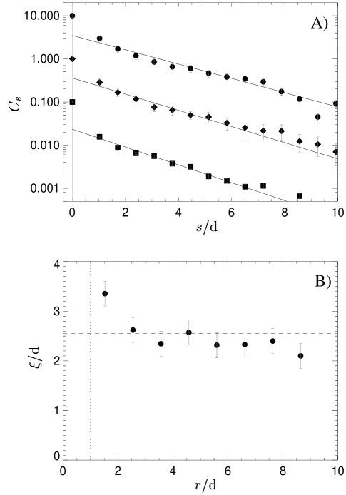
FIG. 7.: Spatial correlations and correlation lengths. (A) The correlation $C_{s}(s,r)$ of the velocity fluctuations of two particles (defined in Eq. 5 in the text) at the same radius $r$ as a function of their separation $s$ for particles at distances from the inner wall of 2.5d (circles), 5.6d (diamonds), and 8.6d (squares). The curves were normalized such that $C_{s}(s=0)=1$, however they have been shifted vertically for clarity. Fits to exponentials for the data $s/d>0$ are shown, and the slopes are used to calculate the correlation length $\xi/d$ as shown in (B). (Note that, for clarity, not all curves were shown in (A).) The correlation length is seen to be nearly constant outside the primary shear zone and somewhat larger very close to the inner wall. The average of the data for $r/{\rm d}>3$ is shown as the horizontal dashed line.

The slopes of the curves in Fig. 7A give the correlation length at each radius, $\xi(r)$, as shown in Fig. 7B. This correlation length is found to be a constant, $\xi=(2.2\pm 0.1){\rm d}$, outside the primary shear zone. Within the primary shear zone $\xi(r)$ is seen to increase to a value of nearly $3.5{\rm d}$ for the innermost particles. This indicates that particle move in larger clusters near the inner wall than at larger $r$.

Time correlations

In addition to spatial correlations, temporal correlations are indirectly visible in videos as well as in particle velocity traces such as those shown in Fig. 4. To extract the characteristic timescale, and spatial dependence of these correlations, I calculated the particle velocity autocorrelation function, $C_{t}(\Delta t,r)$, given by the average correlation of a particle’s velocity fluctuation about its mean at times $t$ and $t+\Delta t$:

$$C_{t}(\Delta t,r)={{\sum(\Delta{v_{\theta}}_{i,t}\Delta{v_{\theta}}_{i,t+\Delta t}+\Delta{v_{r}}_{i,t}\Delta{v_{r}}_{i,t+\Delta t})\delta({1\over 2}(r_{i,t}+r_{i,t+\Delta t})-r)}\over{\sum\delta({1\over 2}(r_{i,t}+r_{i,t+\Delta t})-r)}}-({\delta v(r)}_{\rm cal})^{2}\delta(\Delta t).$$ (6)

The sum is taken over all all particles $i$ and times $t$. As with $C_{s}(s,r)$, the last term is added to eliminate the contribution of noise at $\Delta t=0$. Here I make the assumption that the noise in measuring a particle’s velocity at two different times is uncorrelated.

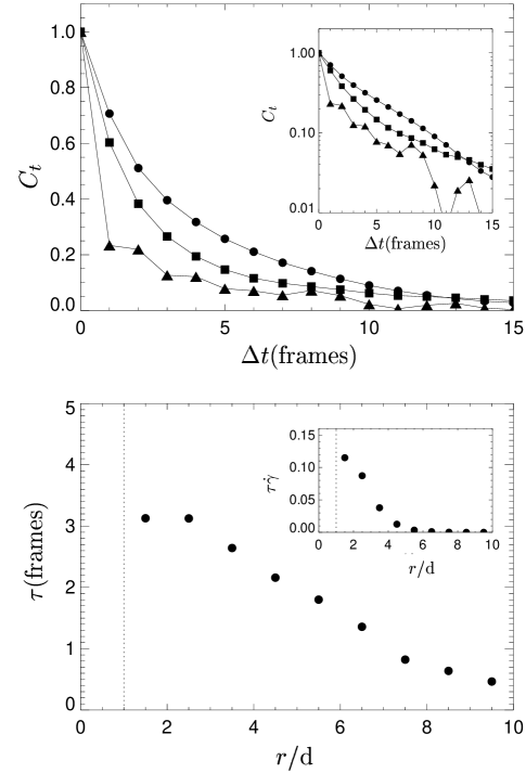
FIG. 8.: The autocorrelation of a particle’s velocity fluctuations over time. The top plot shows the autocorrelation function, $C_{t}(\Delta t,r)$, of a particle’s velocity fluctuations about its mean at times $t$ and $t+\delta t$ for $r/{\rm d}=1.5$ (circles), $r/{\rm d}=4.5$ (squares), and $r/{\rm d}=7.5$ (triangles) as defined in Eq. 6. The noise contribution for $\Delta t=0$ has been subtracted and $C_{t}(\Delta t,r)$ is normalized (for each $r$ value) such that $C_{t}(\Delta t=0,r)=1$. The correlation time $\tau(r)$, defined as the time it takes for $C_{t}(\Delta t,r)$ to fall to $1/e$ for each $r$, is shown in the bottom plot. The inset shows the dimensionless quantity $\tau\dot{\gamma}(r)$, which represents the duration over which particle motion is correlated relative to the timescale over which shear occurs.

$C_{t}(\Delta t,r)$ is shown in Fig. 8A for several distances $r$ from the inner wall. The rate of decay of $C_{t}(\Delta t,r)$ is seen to increase with distance $r$ from the inner wall. The shape of this correlation function is non-exponential (inset to Fig. 8A), indicating that there are correlated processes occurring at multiple timescales. Nevertheless, we can define an effective timescale $\tau(r)$ as the time it takes for $C_{t}(\Delta t,r)$ to fall to ${1\over e}C_{t}(\Delta t=0,r)$. $\tau(r)$ decreases substantially with increasing distance $r$ from the moving wall (Fig. 8B). Thus, particles near the inner wall typically retain their velocity history for several video frames while particles far from the inner wall rarely retain their velocity history for even the interval between two successive frames. The inset to Fig. 8B shows the dimensionless quantity $\tau\dot{\gamma}(r)$, corresponding to the ratio of the correlation time scale and the shear flow time scale.

Fluctuation - shear rate relationship

Having measurements of both the average azimuthal velocity $v_{\theta}(r)$ and the fluctuations of the azimuthal velocity about the mean $\delta v_{\theta}(r)$, I was able to determine the relationship between the fluctuation strength and the shear rate. The shear rate is given by $\dot{\gamma}\equiv\partial v_{\theta}(r)/\partial r$. The fluctuation - shear rate relationship is shown in Fig. 9. The open symbols show the uncorrected data, which exhibit a power-law-like relationship over a small region for large shear, and which asymptote to a constant for smaller shear. The noise floor for $\delta v_{\theta}(\dot{\gamma})$ is calculated from the calibration curves $\delta v_{\theta}(v_{\theta})$ as shown in the inset to Fig. 6. This noise floor is shown by the dotted line in Fig. 9. For smaller shearing rates, the fluctuations $\delta v_{\theta}$ are dominated by the measurement noise. After the noise contribution was subtracted [36] (solid symbols), the overall power law shape of the curve is seen to extend into the smaller shearing region (ie. larger $r$). The dashed line shows a fit of the high-shearing-rate portion of the curve to a power law, with a measured slope $\alpha=0.52\pm 0.04$. This fit is consistent with the entire range of data.

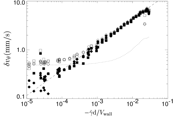
FIG. 9.: Relationship between the fluctuations in the azimuthal velocity and shear rate. The RMS fluctuations of the azimuthal velocity component about its mean, $\delta v_{\theta}(r)$, are plotted against the shear rate $\dot{\gamma}(r)\equiv\partial v_{\theta}(r)/\partial r$ for three different experiments (open symbols). The noise floor for $\delta v_{\theta}$ is shown by the dotted curve, revealing that $\delta v_{\theta}$ is saturated by the noise floor at low shear rates. After removing the contribution of the noise floor to $\delta v_{\theta}$ [36] (solid symbols), I found that the data is well-fit by a power law (dashed line), with a slope of $\alpha=0.52\pm 0.04$.

Shear rate - density relationship

Using the measurements of the material packing fraction, $\rho(r)$, and material velocity, $v(r)$, for this system, the relationship between the shearing rate, $\dot{\gamma}(r)$, and packing fraction, $\rho(r)$, was readily obtained (Fig. 10). The curve is parametrized by $r$, with the smallest $r$ value having low density and high (negative) shearing rate. The line segments connecting data points reflects the path followed as $r$ is increased. Both $\rho$ and $\dot{\gamma}$ oscillate with increaseing $r$. Note that while it is not visible on this figure, $\dot{\gamma}$ is varying by more than three orders of magnitude. For $r$ above 6 particle diameters, $\dot{\gamma}$ is nearly zero on this figure although $\rho$ is still oscillating significantly. While one may approximate this as a linear profile, there are strong oscillations on the single-grain lengthscale throughout the cell.

FIG. 10.: Relationship between the shear rate and packing fraction. The shear rate $\dot{\gamma}{\rm d}/V_{\rm wall}$ is plotted against the packing fraction $\rho$. $V_{\rm wall}=23{\rm mm/s}$ as with all video tracking experiments described here. Points connected by line segments correspond to data points at neighboring values of $r$, which parameterizes both quantities. The lower left data point corresponds to smallest $r$, while large $r$ values have shear rates approaching 0. For larger values of $r$, the shear rate is nearly 0 on this linear plot, however the density continues to oscillate substantially. Note that the three datapoints with largest $\rho$ correspond to the data in Fig. 3 near the outer wall that exceeds the random close pack density in 2D, and are likely caused by layering near the outer cylinder wall.

Discussion

Average flow properties

The average velocity, $v_{\theta}(r)$, was found to be very similar to that previously obtained [10] for roughly monodisperse mustard seeds in the same cell. For all data, Eq. 2 provided an excellent fit. The nearly monodisperse bearing balls were best fit using $\lambda=(2.1\pm 0.2){\rm d}$ and $\sigma=(4.7\pm 0.4){\rm d}$ while the mustard seeds were fit by $\lambda=(2.5\pm 0.2){\rm d}$ and $\sigma=(4.1\pm 0.3){\rm d}$. The similarity in the fitting parameters for these two experiments supports the previous observation that the lower surface has a similar flow profile to the bulk and indicates that the small polydispersity of the mustard seeds does not have a dramatic effect on the overall flow behavior. Although it was not measured in this set of experiments, I expect that this form of the velocity profile is independent of shearing rate for low shearing rates and extends into the bulk of the material, as was previously observed with mustard seeds.

This velocity profile is qualitatively similar to that found by the Duke group for slightly bidisperse disks in 2D [13, 6] and by the Haverford/Penn group for the top surface of a 3D system of glass spheres [16]. Although a fitting form for $v_{\theta}(r)$ was not given for the Haverford/Penn data for glass spheres, inspection of Fig. 5 in [16] reveals that the overall shape of $v_{\theta}(r)$ exhibits curvature (on a log-linear plot) similar to what we observe in the inset to Figs. 2b and 3a. However, the overall velocity gradient across the shear band is dramatically smaller: $v_{\theta}(r)$ in Fig. 3 changes a factor of 1000 between the inner wall and $r=10{\rm d}$ while in the experiment by Bocquet et al. it drops by only a factor of 50 over the same interval. It is possible that this difference is attributable to the difference between the top surface and the bulk. I note, however, that experiments on steel spheres by Bocquet et al. have a rate of decay similar to my experiments on steel spheres. Thus, it is also possible that this difference is attributable to the large polydispersity (diameters range from 0.55 to 0.95 mm) of the glass spheres used by Bocquet et al. In the 2D experiments by the Duke group, the velocity $v_{\theta}(r)$ decays much more quickly than in our experiments. It is not surprising that the 2D experiments differ because they are under a constant volume boundary condition which causes the overall behavior of the system to vary strongly with packing fraction [13, 38]. The steep packing fraction gradient at low $r$ is likely to give rise to the steep velocity gradient.

A large degree of particle layering is observed in the distribution of particle center positions $\rho_{c}(r)$ (Fig. 3B). As discussed in [10], this layering is the source of the exponential term in the velocity profile (Eq. 2). The calculated material packing fraction $\rho(r)$ in Fig. 3C is a 2D quantity in that it is the number of particles per unit area along the lower surface of the cell. This makes quantitative comparison with the previously measured packing fraction for mustard seeds (reproduced in Fig. 2D) inside the bulk difficult. However, the two are qualitatively very similar. Oscillations in $\rho(r)$ are seen to correspond to layering of the particles. The average packing fraction gradually increases with distance from the inner wall. The overall form of $\rho(r)$ appears to be approaching $\rho_{\rm rcp}^{\rm 2D}$. The oscillations in the packing fraction are highly significant, with $\rho_{\rm rcp}^{\rm 2D}-\rho(r)$ typically varying by a factor of 2 over any interval the size of a single grain.

Although it is widely accepted that the packing fraction of a granular material determines, in part, the ease at which it can shear, the relationship between the local shearing rate, $\dot{\gamma}(r)$, and local packing fraction, $\rho(r)$, had not been previously measured to my knowledge. The observed relationship between these two quantities (Fig. 10) reveal that the overall shape is roughly linear for small $r$. This is consistent with the predictions of Bocquet et al. [16]. Large oscillations in $\rho(r)$ and $\dot{\gamma}$ give rise to a substantial degree of variation from the linear form, however. This emphasizes that these quantities are varying significantly on sub-particle lengthscales and suggests that coarse-graining of these quantities may not capture the full behavior of the system.

Fluctuations

The RMS fluctuations of the velocity components about their mean were found to show significant deviation from pure exponential behavior. Instead, $\delta v(r)$ was well-fit by a Gaussian centered on $r=0$ (Eq. 2). The smooth downward curvature seen in the fluctuation profiles, $\delta v_{r}(r)$ and $\delta v_{\theta}(r)$, appears to be in contrast to the form proposed by the Haverford/Penn group [16]. They predict fluctuation profiles that are constant for $r<r_{w}$, and fall off as $\delta v\sim{\rm cosh}({H-y\over{\rm const}})$ for $r>r_{w}$, where $r_{w}$ is a fitting parameter. This form has an elbow at $r_{w}$ and a concave up shape for $r>r_{w}$, in contrast to our observations. Careful observation of Fig. 5 in ref. [16] suggests that the fluctuation profiles found in the Bocquet experiments on glass spheres may also be concave down.

The relationship between the fluctuation strength, $\delta v_{\theta}(r)$, and the shear rate, $\dot{\gamma}(r)$, is consistent with a power-law (see Fig. 9): $\delta v_{\theta}\propto\dot{\gamma}^{\alpha}$ with $\alpha=0.52\pm 0.04$. Since the fluctuation strengths are nearly identical in the radial and azimuthal directions (as shown in Fig. 6), this can be expressed in terms of an effective granular temperature, $T\equiv m{(\delta v)}^{2}$, obtaining $T\propto\dot{\gamma}^{2\alpha}$. With the measured value for $\alpha$, these results are consistent with $T\propto\dot{\gamma}$.

Several theories make predictions about the shear-fluctuation relationship with which these results can be compared. Granular kinetic theory for fast, dilute flows predicts that $\dot{\gamma}\propto\delta v\propto\sqrt{T}$ for steady shear flow [39]. This is inconsistent with our observations for slow, dense flows. This inconsistency is not surprising, as several of the assumptions of kinetic theory do not hold for slow, dense flows. The modified hydrodynamic model of Bocquet et al. predicts $\delta v\propto\dot{\gamma}^{\alpha}$, although it makes no prediction for the value of $\alpha$ other than $\alpha<1$. They measure $\alpha=0.4$ and point out that the 2D experiments of the Duke group have $\alpha=0.5$. Thus, the observed relationship between the shear rate and fluctuation amplitude is in agreement with these other experiments and the modified hydrodynamic model. From this it is clear that kinetic theory is unable to capture the behavior in the slow, dense limit unless the pair correlation function $g(r)$ (and thus the viscosity) for a dense material is used, as done by Bocquet et al.

Correlations

The coherent motion of neighboring particles observable in videos of the motion and trajectory plots, is quantified by the spatial correlation function $C_{s}(s,r)$ (Fig. 7). The exponential decay of $C_{s}(s,r)$ suggests a process due to nearest neighbor interactions of particles, such as a string of particles in contact, correlated over a typical length $\xi$.

The correlation length $\xi(r)$ was found to be essentially constant away from the inner wall, suggesting the local material property, as it pertains to coherent motion of particles, is uniform in this region. One may speculate that the correlation length $\xi$ may be determined by the randomness of particle contact angles. Knowledge of the direction of motion of a given particle is quickly lost by its neighbors in a disordered pack. In this picture, the constant value of $\xi(r)$ would correspond to a uniformly disordered pack. Only inside the first moving layers, closest to the wall, the correlation length is found to increase indicating that particles are moving in larger clusters. This may be a consequence of particle layering. The particles tend to line up with contacts in the same direction as their primary motion, possibly leading to an increased correlation length.

The coherence of particle motion in time was also originally evident in videos of the shear flow and particle trajectories. Plots of the velocity traces for individual particles (Fig. 4) reveal the intermittancy of the flow. Distinct motion events are visible at all regions of the cell. In many cases, sudden changes in velocity indicate that a particle suddenly became jammed or freed. While the interval between motion events was observed to increase substantially with distance $r$ from the inner wall, the duration and speed of each motion event appeared to decrease only slightly with $r$.

The correlation of a particle’s velocity fluctuations over time, $C_{t}(\Delta t,r)$ decays with a correlation time $\tau(r)$ which varies with $r$. For small $r$, the velocity persists for several time frames (about 15 ms) for an inner cell wall speed of $v_{\rm wall}=23{\rm mm/s}$. This corresponds to a correlation over the time it takes the inner wall to move by 0.35d. Note that while the correlation time $\tau(r)$ is decreasing with $r$, the characteristic timescale for shear flow, $\dot{\gamma}^{-1}$, is increasing with $r$. Thus, ratio of the correlation timescale to the shear timescale, $\tau\dot{\gamma}(r)$, decays very quickly with $r$ indicating that the flow is not uniformly slowing down with increasing $r$. The decrease in correlation time $\tau(r)$ with $r$ may be caused by multiple effects including the speeding-up of motion events, the weakening magnitude of the events, and the increased rarity of motion events. However, it is clear from looking at velocity-time traces such as those shown in Fig. 4 that the primary change in behavior is that the interval between motion events becomes very large at large $r$. While one may expect the correlation time $\tau(r)$ to increase with $r$ since the flow is occuring over longer timescales, the opposite trend is observed. With increasing $r$, the events occur increasingly quickly and at increasingly long intervals.

Summary and Conclusion

I found that fluctuations in the velocities of two particles at radius $r$ are correlated within a characteristic lengthscale $\xi(r)$. Away from the moving inner wall, the correlation length is $\xi=(2.3\pm 0.1){\rm d}$, while near the moving wall the correlation length increases to $\xi\approx 3.5{\rm d}$. Correlations in time are also observed, both through velocity traces as well as direct calculation of the correlation function, $C_{t}(\Delta t,r)$. The correlation time, $\tau$, was found to be 13 ms near the moving inner wall and decreases with $r$. Distinct motion events, intervals over which a previously stationary or slow-moving particle moves more quickly before slowing down or coming to rest, were also directly observed in velocity traces. The interval between motion events was observed to increase quickly with distance from the inner wall. The observed intermittancy and velocity correlations are reminiscent of that observed in force chains in a similar geometry by Behringer and Howell [6], which suggests force chains may play a role in the dynamics.

Having directly measured the velocity, velocity fluctuations, and density within the same system, I was able to compare my observations with the predictions of hydrodynamic and kinetic theories of granular flow. I measured a power law relationship between shear rate and fluctuation amplitude, $\delta v\propto\dot{\gamma}^{\alpha}$, with $\alpha=0.52\pm 0.04$. This form is consistent with the hydrodynamic theory of Bocquet et al. and experiments by this group [16], although it is inconsistent with simple kinetic theory without corrections for high density packs which predicts $\alpha=1.0$ [39]. The overall form for the azimuthal velocity fluctuations about their mean, $\delta v_{\theta}(r)$, was found to be Gaussian in shape, in contrast to the cosh form predicted by the hydrodynamic theory.

The relationship between the shear rate and packing fraction can be approximated by a linear relationship close to the shearing wall. However, the variations from this form are quite large due to the strong oscillations in both the packing fraction and the shear rate with distance from the inner cell wall. This emphasizes that the behavior on sub-particle lengthscales is very different from that on larger scales, and that the coarse-grained approach used in kinetic and hydrodynamic theories is unable to describe the behavior on this scale.

While some aspects of the flow are described within existing theories, many of the observations reported are still not understood. The Gaussian component to the velocity profile, $v_{\theta}(r)$, indicates that the inner cylinder wall, $r=0$, plays an important role in the flow behavior. As $r$ increases from this wall, the shape of the azimuthal velocity distributions, $P(v_{\theta})$, varies from roughly Gaussian to exponential in shape (Fig. 5). Also, although the time for flow to occur becomes very large at large $r$, the correlation time $\tau(r)$ decreases with $r$ and changes only by a factor of six (Fig. 8), as the interval between motion events becomes very large but the duration of motion events does not change dramatically (Fig. 4). Together, these results suggest the presence of an underlying mechanism of shear transmission from the inner wall ($r=0$) outward in a stochastic fashion along intermittent chains of contact.

REFERENCES

- [1] H. M. Jaeger, S. R. Nagel, and R. P. Behringer, Physics Today 49, 32 (1996).
- [2] R. A. Bagnold, Proc. Royal Soc. London 225, 49 (1954).
- [3] S. Ogawa, A. Umemura, and N. Oshima, J. Appl. Math. Phys. 31, 483 (1980).
- [4] J. T. Jenkins and S. B. Savage, J. Fluid Mech. 130, 187 (1983).
- [5] D. Howell and R. P. Behringer, in Powders & Grains 97, edited by R. P. Behringer and J. T. Jenkins (Balkema, Rotterdam, 1997), pp. 337–340.
- [6] D. Howell and R. P. Behringer, Phys. Rev. Lett. 82, 5241 (1999).
- [7] See, for example, the videos at http://www.phy.duke.edu/ dhowell/research.html and http://mrsec.uchicago.edu/granular.
- [8] A. J. Liu and S. R. Nagel, Nature 21, 396 (1998).
- [9] C. S. O’Hern, S. A. Langer, A. J. Lui, and S. R. Nagel, Phys. Rev. Lett. 8, 111 (2001).
- [10] D. M. Mueth et al., Nature 406, 385 (2000).
- [11] D. W. Howell, (private communication).
- [12] R. Khosropour, J. Zirinsky, H. K. Pak, and R. P. Behringer, Phys. Rev. E 56, 4467 (1997).
- [13] C. T. Veje, D. W. Howell, and R. P. Behringer, Phys. Rev. E 59, 739 (1999).
- [14] W. Losert, L. Bocquet, T. C. Lubensky, and J. P. Gollub, Phys. Rev. Lett. 85, 1428 (2000).
- [15] A. Karion, Ph.D. thesis, California Institute of Technology, Pasadena, California (USA), 2000.
- [16] L. Bocquet et al., cond-mat/0012356 (unpublished).
- [17] For some examples of 3D imaging of Couette flow with X-ray tomography, see http://mrsec.uchicago.edu/granular/index.html.
- [18] G. T. Seidler et al., PRE 62, 8175 (2000).
- [19] E. Fukushima, Ann. Rev. Fluid Mech. 31, 95 (1999).
- [20] M. Nakagawa, S. A. Altobelli, A. Caprihan, and E. Fukushima, in Powders & Grains 93, edited by C. Thornton (Balkema, Rotterdam, 1993), p. 383.
- [21] E. E. Ehrichs et al., Science 267, 1632 (1995).
- [22] J. D. Seymour, A. Caprihan, S. A. Altobelli, and E. Fukushima, PRL 84, 266 (2000).
- [23] A. Caprihan and J. D. Seymour, J. Magn. Reson. 144, 96 (2000).
- [24] In 2D Couette systems, sheared under constant volume conditions, rough particles such as pentagons may actually produce a velocity profile that is very well fit by a pure exponential. (Dan Howell and Bob Behringer, private communication).
- [25] G. Debregeas and C. Josserand, Europhys. Lett. 52, 137 (2000).
- [26] Note that the work of Losert et al. defines as the outer edge of glued particle layer, while we define as the inner edge of the glued particle layer. Thus a Gaussian profile centered on in our experiments, as seen for disordered materials, is equivalent to a Gaussian profile centered on for the experiments of Losert et al.
- [27] P. K. Haff and B. T. Werner, Powder Technol. 48, 239 (1986).
- [28] C. Josserand, Europhys. Lett. 48, 36 (1999).
- [29] A. V. Tkachenko and V. Putkaradze, submitted to PRE (unpublished).
- [30] Commonly available glass spheres are molded and typically have sphericities of about 95%. Gluing these glass spheres to a plate and rotating the plate at constant velocity shows an apparent relative motion of the particles easily visible to the eye as if the particles were not actually glued in place. This increases the uncertainty in each velocity measurement substantially, raising the noise floor for the fluctuation measurements, and increasing the noise level in the correlation measurements substantially.
- [31] The maximum achievable precision for an annulus of radius pixels is approximately pixels. The realizable precision however may be limited by the quality of the optics, sphericity of the particles, pixel noise in the camera, and other factors.
- [32] I would like to thank Wolfgang Losert who pointed out the benefits achieved from defocussing the optics.
- [33] D. R. Nelson and M. Rubinstein, Phil. Mag. A 46, 105 (1982).
- [34] I used the band-pass filtering, feature finding, and particle tracking routines written by David Grier and John Crocker for these steps.
- [35] D. Bideau, A. Gervois, L. Oger, and J.-P. Toadec, J. Phys. France 47, 1697 (1986).
- [36] Noise adds to the signal in quadrature for the fluctuations, , and the correlation functions, and .
- [37] Correlations between particle velocities at seperate times or positions are robust against noise, since the noise is uncorrelated. However for , velocity measurement noise is additive in . To eliminate this contribution, the average measurement noise squared, , from the calibration experiment is subtracted from .
- [38] D. W. Howell, R. P. Behringer, and C. T. Veje, Chaos 9, 559 (1999).
- [39] P. K. Haff, Journal of Rheology 30, 931 (1986).