Equilibrium valleys in spin glasses at low temperature

Abstract

We investigate the $3$-dimensional Edwards-Anderson spin glass model at low temperature on simple cubic lattices of sizes up to $L=12$. Our findings show a strong continuity among $T>0$ physical features and those found previously at $T=0$, leading to a scenario with emerging mean field like characteristics that are enhanced in the large volume limit. For instance, the picture of space filling sponges seems to survive in the large volume limit at $T>0$, while entropic effects play a crucial role in determining the free-energy degeneracy of our finite volume states. All of our analysis is applied to equilibrium configurations obtained by a parallel tempering on $512$ different disorder realizations. First, we consider the spatial properties of the sites where pairs of independent spin configurations differ and we introduce a modified spin overlap distribution which exhibits a non-trivial limit for large $L$. Second, after removing the $Z_{2}$ ($\pm 1$) symmetry, we cluster spin configurations into valleys. On average these valleys have free-energy differences of $O(1)$, but a difference in the (extensive) internal energy that grows significantly with $L$; there is thus a large interplay between energy and entropy fluctuations. We also find that valleys typically differ by sponge-like space filling clusters, just as found previously for low-energy system-size excitations above the ground state.

]

I Introduction

In the past two decades there has been a large amount of theoretical, experimental, and numerical work on spin glasses (see for example [1, 2], and references therein). Two different points of view have dominated the frameworks used by most researchers. On one side, there is the idea that mean field features [3, 4, 5, 6, 7, 8], that are astonishingly different from those encountered in systems without frustration, are relevant in realistic, finite dimensional spin glasses. On the other side, there is the expectation that the (non-trivial) extension [9, 10] of scaling ideas to these frustrated systems should be the correct framework for short range spin glasses. The results contained in this note will give support to the point of view that many features of the finite dimensional Edwards-Anderson (EA) [11] spin glasses are common to the ones of the mean field Parisi solution and are well described in terms of the Replica Symmetry Breaking (RSB) approach. This point of view is already supported by a large number of numerical simulations and by studies of ground states. Indeed, numerical simulations indicate, among other features, that the EA model has an average overlap probability distribution $P(q)$ which is broad in the thermodynamic limit, signaling (continuous) RSB (see [12] and references therein). Similarly, ground state computations [13, 14, 15, 16, 17, 18] show that the energy landscape of the EA model is characterized by system-size valleys whose excitation energies remain of order one in the infinite volume limit. The consequence of this property on the system at temperature $T>0$ is likely to be RSB. This is typically expected to imply that for a given instance of the disorder (one given realization of the quenched random couplings) spin configurations will cluster into multiple “valleys”, not related by the up-down symmetry (there is no magnetic field so we shall always work modulo the $\pm 1$ symmetry).

The purpose of this work is to study the $3$-d EA model at low temperature, and to characterize its valleys, both thermodynamically and for their position-space (i.e., spatial) properties. Among other things, we ask whether valleys having $O(1)$ free-energy differences have similar energies and entropies; if not, RSB implies that the fluctuations in these quantities must nearly cancel. Also, what are the typical differences among valleys? How does one go from one valley to another? Before addressing these questions, we have to be far more specific in defining a valley. Our definition is algorithmic, based on a method for clustering configurations according to their spin overlaps (or equivalently according to their Hamming distances). Such a clustering scheme has been used successfully by Hed et al. [17] for analyzing spin glass ground state configurations. By applying such a clustering algorithm, we determine at a given temperature the “valleys” that characterize each disorder realization. Then we compute various statistical properties of these valleys and of their associated TAP-like states. Interestingly, the picture obtained from looking at $O(1)$ energy system-size excitations above the ground state [18] also applies to our finite temperature valleys. One goes from one valley to another by flipping system-size clusters of spins that are space filling and topologically highly non-trivial: this justifies calling them spongy clusters [19].

The outline of this paper is as follows. First we specify how our equilibrium configurations were generated. Then, given two such configurations, we consider various ways to compare them with a special attention on topological properties of the set of spins where they differ. We construct the clusters of these spins and classify them into sponge-like, droplet-like, or neither of these. Our data indicate that, if the statistics of such topological events are monotonic with $L$, sponge-like events arise with a strictly positive probability in the large $L$ limit. Then we describe how we define the valleys into which we will cluster our equilibrium configurations (we give additional details about the clustering algorithm in the appendix). Not surprisingly, configurations assigned to significantly different valleys nearly always have sponge-like differences, i.e., they do not differ in localized, droplet like areas, but in a diffuse set of sites. We compute the (extensive) internal energy of each valley: we find that this quantity fluctuates dramatically from valley to valley, growing very clearly with the lattice size $L$. Finally we consider the properties of the TAP-like states associated with the valleys. We find that again the difference among different TAP-like states is typically given by a spongy cluster, just as in the zero temperature case. We also study the link overlap distribution among these states.

II The model and its numerical simulation

We consider the $3D$ Edwards-Anderson (EA) spin glass model, whose Hamiltonian is

$$H=-\sum_{\langle ij\rangle}J_{ij}S_{i}S_{j}\ ,$$ (1)

where $\langle ij\rangle$ indicates that the sum is over nearest neighbors. We work on simple cubic lattices with periodic boundary conditions and zero magnetic field. The quenched couplings $J_{ij}$ are independent random variables that can take the two values $\pm 1$ with equal probability $1/2$. In this study we have used spin configurations at $T=0.5$. (Note that $T_{c}\simeq 1.1$.) We will present data taken on lattices of linear size $L=6$, $8$ and $12$.

We rely on a parallel tempering updating scheme (see for example [20] and references therein) that is very effective for simulating EA spin glasses. The different temperatures used in the runs are uniformly spaced. We use $19$ temperature values going from $T_{min}=0.5$ to $T_{MAX}=2.3$ on the $L=6$ lattices, $49$ temperature values going from $T_{min}=0.5$ to $T_{MAX}=2.1$ on the $L=8$ lattices, and $64$ temperature values going from $T_{min}=0.5$ to $T_{MAX}=2.075$ on the $L=12$ lattices. We have checked in detail that we reach a very good thermalization according to all the usual tests [20]: the acceptance ratio of the tempering sweeps is high (always of order $0.7$), the permanence histograms are very flat, and observables look very constant when plotted as a function of the log of the elapsed Monte Carlo time. In addition, we have checked that on individual disorder instances the $\pm 1$ symmetry of $P_{J}(q)$ is very well satisfied, see for example figures 1 and 2. In short, since we have used very long MC runs with very conservative and safe choices of the parameters, thermalization seems to be complete.

For each disorder instance and lattice size, we perform the parallel tempering independently on two (sets of) replicas. For each, we first run $10^{6}$ MC sweeps just to reach thermalization; a sweep consists of $L^{3}$ trial spin flips and one tempering $\beta$ trial update. Following that, we run for $1.1\cdot 10^{6}$ MC sweeps to gather (equilibrium) statistics. During these sweeps we save $1100$ spin configurations, that is one every $1000$ MC sweeps, giving a total of $2200$ equilibrium configurations for that disorder sample. These are the configurations that are used for the analysis described in the rest of this paper. The runs to generate these configurations took on the order of $2$ weeks of machine time on a dedicated Linux cluster based on $16$ Pentium II $450MHz$ processors.

For each lattice size ($L=6$, $8$, and $12$), we thus have $16\times 32=512$ different disorder samples (the factor $32$ comes from the use of multi-spin coding on each of the $16$ machines), and a total of $2\times 1100$ equilibrium spin configurations for each disorder sample.

III Droplet and sponge differences of equilibrium configurations

Each spin configuration $C$ appears at equilibrium, at temperature $T$, with probability $P_{B}(C)=Z_{J}^{-1}\exp(\frac{-H(C)}{T})$ (where $Z_{J}$ is the partition function which normalizes the Boltzmann weight for that instance). Consider a pair of spin configurations $C^{(1)}$ and $C^{(2)}$, selected independently according to their à priori probability, and let $G$ be the set of sites where the spins of the two configurations differ. One defines the spin overlap by

$$q(C^{(1)},C^{(2)})=\frac{1}{N}\sum_{i=1}^{N}S_{i}^{(1)}S_{i}^{(2)}\ ,$$ (2)

where in our $3$-d case $N=L^{3}$. If $|G|$ is the cardinality of $G$, then $q=1-2|G|/N$. In figure 1 we show an example (for $L=12$) of a distribution $P_{J}(q)$ of overlaps for one realization of the disorder (the dotted curve), and with the solid curve we show the distribution averaged over the disorder, that is over our $512$ disorder samples. Because of the up-down symmetry, in the rest of this work we will only look at the $q\geq 0$ part of the support, and we will ignore the part for negative $q$ values. For the disorder instance used in figure 1, most of the overlaps are close to the two values associated with the positions of the two peaks of $P_{J}(q)$. This suggests that in this instance the spin configurations fall into two “valleys”, as will be confirmed later. In figure 2 we consider a different disorder instance where $P_{J}(q)$ has three peaks (always in the $q>0$ sector). Because of this kind of behavior, we should investigate what happens when we cluster the configurations according to their mutual overlaps; however, before doing so, let us first discuss how two equilibrium configurations differ spatially.

FIG. 1.: Probability distribution $P_{J}$ of the spin overlap $q(C^{(1)},C^{(2)})$ for a given disorder instance (dotted curve), and its disorder average $P$ (solid curve).

FIG. 2.: As in figure 1, but for a disorder instance that generates three peaks in $P_{J}$ at $q>0$.

When two configurations are in the same valley, we expect them to differ only by droplet-like objects; the set of spins $G$ forming their difference should consist of small clusters. On the contrary, when considering configurations in two different valleys, we expect $G$ to contain a large and topologically non-trivial cluster. To quantify this, we follow reference [18] and declare $G$ to be sponge-like if it and its complement wind around the lattice in all three directions, whereas we call it droplet-like if it does not wind around any of the three directions of the lattice. Finally we label intermediate the other cases of windings. Our data show very clearly a strong correlation between the (relative) size of $G$ and its topological class: the larger ${|G|}/{L^{3}}$, the more likely it is to be sponge-like. Do sponge-like differences between equilibrium configurations survive in the large $L$ limit? In table I we give the probabilities of the three topological classes as a function of the lattice size. Just as in the $T=0$ energy landscape studies [18], the frequencies of sponge-like events increases as $L$ increases, suggesting that in the limit $L\to\infty$ equilibrium configurations differ by sponge-like clusters with a strictly positive probability.

TABLE I.: Probability of each of the $3$ topological classes for differences of independent spin configurations.

L	sponge-like	intermediate	droplet-like
6	$0.082\pm 0.005$	$0.157\pm 0.007$	$0.761\pm 0.010$
8	$0.104\pm 0.006$	$0.166\pm 0.007$	$0.730\pm 0.010$
12	$0.117\pm 0.007$	$0.160\pm 0.006$	$0.723\pm 0.010$

Coming back to the distribution of overlaps, let us decompose $P(q)$ into the sum of three densities, one for each topological class:

$$P(q)=\rho_{s}(q)+\rho_{d}(q)+\rho_{i}(q)\ ,$$ (3)

where $\rho_{s}$ is the sponge density, $\rho_{d}$ the droplet density, and $\rho_{i}$ the intermediate density. (A different decomposition based on valleys has been introduced by Hed et al. [21]; our method has the great advantage that it does not rely on any clustering into valleys and is thus parameter-free.) Now consider only those pairs of configurations where $G$ is sponge-like: we show in figure 3 the density distribution $\rho_{s}$ of the overlaps belonging to this topological class. The main trend is the widening of the distribution’s support: sponge-like $G$’s can occur for increasing values of $q$ as $L$ grows. Other than that, for small $q$, $\rho_{s}$ is stable when $L$ increases from $6$ to $12$: this constitutes further numerical evidence for replica symmetry breaking in the three-dimensional EA model.

FIG. 3.: The density distribution $\rho_{s}$. This is the restriction of $P(q)$ to overlaps associated with configurations $C^{(1)}$ $C^{(2)}$ having sponge-like differences.

IV Clustering equilibrium configurations

We want to give an appropriate definition of a valley. One would like a valley to be a connected region in phase space that contributes a finite measure to the partition function (this statement can be made precise by coarse graining the phase space). Configurations belonging to the same valley are then expected to be close (i.e., they have a large overlap), while configurations belonging to different valleys are expected to be far (small overlap). Now, in more precise terms, given a collection of equilibrium configurations, we seek to cluster them into families which hereafter we shall refer to as valleys. Although this kind of classification problem is generally ill-posed, one expects good clustering methods to lead to nearly identical results when the valleys are well separated. Such an “ideal” case arises in models with one-step RSB: there, the overlap between two equilibrium configurations converges in the thermodynamic limit to one of two possible values, so assigning configurations to clusters is straight-forward.

In the case of continuous RSB, the situation is slightly ambiguous because in the thermodynamic limit we expect that there will be some hierarchical organization of the states: there will be valleys inside valleys inside valleys… Nevertheless, it is still meaningful to define valleys, as long as the splitting of valleys into sub-valleys is not relevant for the observables considered. If that is indeed the case, one can in fact allow for valley sub-divisions ad infinitum as was done by Hed et al. [17]: those authors clustered ground state configurations in the $3$-d $\pm J$ EA model, letting the sub-valley sizes become arbitrarily small. Since our goal here is to focus on well separated valleys, we construct our valleys up to some cut-off overlap value $q^{*}$; in effect, all sub-valleys with overlaps larger than $q^{*}$ are lumped together. After, we will check by using different values of $q^{*}$ that our findings are not sensitive to that cut-off; this can be so of course only when considering observables associated with overlaps smaller than that cut-off.

For completeness, we give here a high-level description of our clustering method. The appendix gives some details about the algorithm itself (a similar approach was defined by Iba and Hukushima [22]). Conceptually, our assignment of equilibrium configurations to a given valley is motivated by the TAP states[23] arising in the mean field picture. Each of our valleys will be associated with a “TAP-like” state which for our purposes is just a set of magnetizations, one for each site. In analogy with TAP states, these magnetizations are the thermal averages of the spin variables, restricted to configurations belonging to the valley of interest; this is like using a “finite volume equilibrium state” to define the TAP states. Thus, given the set of configurations assigned to a valley, we compute the magnetization $m_{i}$ at site $i$ by finding the mean of the values of the $S_{i}$ over these configurations. If we want to have $M$ valleys, we are to find $M$ TAP-like states; algorithmically, we find these $M$ states and their associated valleys by iteration. The self-consistency conditions are that:

1. the TAP-like state of valley $k$ is defined by the magnetizations $m_{i}$ of that valley;

2. a configuration belongs to the valley $k$ if the TAP-like state nearest to it is number $k$ (the nearness is measured by the overlap) and if that overlap is greater than $q^{*}$.

If $q^{*}$ is close to $1$ only very similar configurations will be included into the same valley; on the contrary, if $q^{*}$ is small most of the time all the configurations will be assigned to just one valley. Intuitively, one can think of $q^{*}$ as being a resolution; as one increases $q^{*}$, valleys get resolved into sub-valleys, and as $q^{*}\to 1$, one reaches the limit where each valley corresponds to a single spin configuration.

Our self-consistent procedure does not generally determine the clustering uniquely, but as was said before, any reasonable clustering algorithm should do well if the valleys are sufficiently separated (that is the case we want to consider in this work). In practice we find the valleys (and their TAP-like states) iteratively: we start by defining a first valley, then when possible and needed we add and define a second valley, and so on. For a given value of the cut-off $q^{*}$, one clusterizes more and more of the configurations when increasing the number of TAP-like states. One stops the construction when any of the following conditions are met: (i) all spin configurations have been assigned to valleys; (ii) a maximum number of valleys (namely ten in our code) has been reached; (iii) increasing the number of TAP-like states would lead to too similar valleys, that is some of the overlaps of the TAP-like states would become greater than $q^{*}$.

At the end of the procedure, the algorithm gives us valleys (families of configurations) and their associated TAP-like states. Not surprisingly, for instances where the clustering leads to several sizeable valleys, the $P_{J}(q)$ has several peaks, and the reverse is also true. Furthermore, we checked the property previously mentioned in section III, namely that configurations in valleys with small mutual overlaps usually differ by sponge-like clusters.

To give the reader a bit of intuition about how the algorithm behaves, let us show what happens for the disorder instance used in figure 1. For that instance, there are two peaks in $P(q)$, one near $q=0.6$ and the other near $q=0.8$. Thus we expect to find two valleys with self-overlap close to $0.8$ and whose mutual overlap should be near $0.6$. Recall that $q^{*}$ acts as a resolution; let us then follow the result of the clustering as we go from $q^{*}=0$ (low resolution) to $q^{*}=1$ (high resolution).

For small values of $q^{*}$, the algorithm puts nearly all the configurations into one huge valley. (Recall that we work modulo the $\pm 1$ symmetry; the Hamiltonian has no magnetic field and our clustering procedure respects that symmetry by always working modulo this symmetry. In effect, each configuration can be identified with a pair of opposite configurations.) The self-overlap of the corresponding TAP-like state is quite stable, going from $0.741$ at $q^{*}=0$ to $0.752$ at $q^{*}=0.61$. Then at $q^{*}=0.62$, this big valley breaks up into two sub-valleys. The break-up is accompanied by a discontinuity in the self-overlap: for the largest valley, it jumps to $0.86$. Also, the overlap between the two TAP-like states is $0.61$. This value is no surprise as the algorithm forbids TAP-like states with overlaps greater than $q^{*}$; when new valleys appear, one of the inter-valley overlaps should correspond precisely to the cut-off.

Now we increase $q^{*}$ further. For the range $0.62\leq q^{*}\leq 0.72$, the assignment of the $2200$ configurations to the $2$ valleys is $q^{*}$-independent. Beyond $q^{*}=0.72$, things are qualitatively similar except that a small number of configurations leave these valleys. This can be understood quite simply: the configurations in the valley that are the furthest from the TAP-like center will be pushed out first. Finally, when $q^{*}>0.82$, the largest valley breaks up and we end up with more small valleys. Clearly, once $q^{*}$ is close to $q_{EA}$, one will not keep a small number of valleys; such values of $q^{*}$ should not be used. Even in the case of systems without frustration and disorder, this would lead to multiple valleys.

V Valley-to-valley energy fluctuations

The main goal of this work is to understand how valleys differ; to this end it is convenient, among the $512$ disorder instances we have produced, to focus only on those that give rise to more than one valley. For each instance of that type, the $2200$ equilibrium configurations cluster into two or more valleys as generated by our algorithm. (For the data shown hereafter, the resolution is $q^{*}=0.5$.) However, sometimes one of these valleys will be of very small size, containing $1$ or $2$ configurations. Since we want to investigate typical properties, we have decided to study only valleys of an acceptable size. Quantitatively, we do this by restricting ourselves to the two largest valleys and by demanding that each of them include a substantial fraction of the $2200$ spin configurations.

The analysis we present in this section has been performed using those disorder instances where the two largest valleys together contain at least $80\%$ of the configurations, and the second largest valley at least $20\%$. Out of the $512$ disorder instances, these selection criteria left us with $81$ instances for $L=6$, $91$ instances for $L=8$, and $91$ instances for $L=12$. We have repeated the analysis with different thresholds and have found that our conclusions are unaffected by the change. We now begin by discussing the thermodynamic properties of these valleys, while in the sections thereafter we will focus on the corresponding TAP-like states.

The free-energy $F_{r}$ of a valley $r$ is defined as

$$e^{-F_{r}/T}=\sum{{}^{\prime}}~{}e^{-H(C)/T}\ ,$$ (4)

where $\sum{{}^{\prime}}$ indicates that only those configurations $C$ belonging to valley $r$ are to be included. Note that this sum is the weight of that valley, equal to the valley’s contribution to the partition function $Z_{J}$. Since the Monte Carlo samples configurations according to their Boltzmann factor, it visits the different valleys according to their contribution to $Z_{J}$. Thus, the number of times the Monte Carlo generates a configuration in valley $r$ is proportional to $\exp(-F_{r}/T)$.

For convenience, we order our valleys according to their size (the largest valley includes $|V_{1}|$ configurations, the next largest $|V_{2}|$, and so on). As a result, the valleys are ordered by increasing free-energies. Defining $\Delta F=F_{2}-F_{1}\geq 0$, we can estimate this difference from our data as

$$\exp\left[-\frac{\Delta F}{T}\right]=\frac{|V_{2}|}{|V_{1}|}\ .$$ (5)

In the mean field picture, $\Delta F=O(1)$ with a finite probability at large $L$. It is not difficult to see that our selection criteria impose $\Delta F=O(1)$; what is then relevant is the fraction of disorder instances that pass these selection criteria. These fractions are $15\%$, $17\%$, and $17\%$ for $L=6$, $8$, and $12$. Within the error bars, these fractions are stable, in agreement with the mean field picture.

FIG. 4.: Probability distributions of $\Delta F$, for $L=6$, $8$, and $12$.

Another prediction of the mean field theory is that $\Delta F$ has an exponential distribution, with a slope becoming small as $q^{*}$ decreases. In figure 4 we show the numerical values we have found for the probability distribution of $\Delta F$ at $L=6$, $8$, and $12$. The distribution seems quite insensitive to $L$ and its shape is rather flat. Again we interpret the data as being compatible with the mean field picture.

Each valley can be thought of as a finite volume equilibrium state; intensive observables are expected to have the same values across different valleys, but extensive quantities can very well fluctuate significantly. Let us thus consider the (extensive) internal energy of valley $r$: $E_{r}$ is defined as the average of the energies of the configurations belonging to that valley. We have measured the statistical properties of $\Delta E\equiv E_{2}-E_{1}$. First, we find that the mean of this random variable is positive; that can be understood by saying that since by construction $\Delta F>0$, all other things being equal, one expects $\Delta E>0$.

FIG. 5.: Probability distribution of $\Delta E$, for $L=6$, $8$, and $12$.

Second, the spread of the distribution of $\Delta E$ grows with $L$; this is very visible in figure 5 and is to be contrasted with the behavior of $\Delta F$. To make this point more quantitative, we have calculated the variances of $\Delta E$; these are given in table II, confirming that the distribution of $\Delta E$ broadens as $L$ increases. Third, we find that the linear correlation coefficient of $\Delta E$ and $\Delta F$ is small. This coefficient is defined as

$$C(\Delta E,\Delta F)={\frac{\overline{(\Delta E-\overline{\Delta E})(\Delta F-\overline{\Delta F})}}{\sigma(\Delta E)~{}~{}\sigma(\Delta F)}}\ ,$$ (6)

where $\sigma$ is the standard deviation of the variable of interest and an over-bar stands for the disorder average. The values of $C$ are also given in the table. It would be nice to test the possibility that the variance of $\Delta E$ grows as a power of $L$, but our range of lattice sizes is too small to seriously test this hypothesis. Nevertheless, the picture we extract from our analysis is that these “large” fluctuations in energy must be compensated by similar fluctuations in entropy, otherwise one could not have $\Delta F=O(1)$. Most probably, these fluctuations play a crucial role in all frustrated disordered systems and they deserve further investigation.

TABLE II.: $\Delta F$, mean and variance of $\Delta E$, and correlation coefficient of $\Delta E$ and $\Delta F$.

L	$\overline{\Delta F}$	$\overline{\Delta E}$	$\sigma(\Delta E)$	$C(\Delta E,\Delta F)$
6	0.317	0.418	1.879	0.048
8	0.352	0.364	2.409	0.005
12	0.328	0.771	4.123	0.114

VI Inter-valley differences: spin and link overlaps

We focus here on the relation between spin and link overlaps: are these two fluctuating quantities correlated? A motivation for this question comes from mean field theory where $q_{l}$ becomes a deterministic function of $q$ in the thermodynamic limit. To investigate this possibility, we look at the variance of $q_{l}$ at fixed $q$. There are several approaches: the first considers all fluctuations; the second focuses on instance to instance fluctuations only; the third is based on the fluctuations given by the TAP-like states of our valleys.

Consider the first approach. We take equilibrium configurations at random, and determine (for $q$ in a small range) the distribution of $q_{l}$ for $L=6$, $8$, and $12$. This distribution is averaged over the disorder, and we consider the resulting variance. We find that the variance decreases as one increases $L$; for example, in the bin $0\leq q\leq 0.1$, the standard deviation is $0.043$ at $L=6$, $0.033$ at $L=8$, and $0.028$ at $L=12$. (The other bins give very similar results.) This decrease is unambiguous, and is highly suggestive of an asymptotic decrease to $0$ as $L\to\infty$. Previous work [24] on ground states lead to this same conclusion.

Fluctuations in $q_{l}$ come from thermal noise within a given instance and from instance to instance fluctuations. In a naïve way, assume that the variances add linearly, $\sigma^{2}(q_{l})\approx\sigma_{T}^{2}(q_{l})+\sigma_{J}^{2}(q_{l})$ where the first one is the intra-instance (purely thermal) variance and the second one is the inter-instance variance. The thermal fluctuations are due to thermally excited droplets inside the valleys; these fluctuations are expected to average out in any scenario, so that $\sigma_{T}^{2}(q_{l})\to 0$ at large $L$. The measurements of the previous paragraph show that $\sigma^{2}(q_{l})$ decreases as $L$ grows, but this can happen even if $\sigma_{J}^{2}(q_{l})$ saturates at a positive value. It is thus appropriate to determine the $L$ dependence of $\sigma_{J}^{2}(q_{l})$ by itself. This leads us to our second method whereby we find the mean of $q_{l}$ in a given disorder instance (and for $q$ in a given bin) and then we consider its instance to instance fluctuations. Naturally, the variances now are smaller than in the previous measurements. Is there a sign of saturation? Let us again give our results for $0\leq q\leq 0.1$: at $L=6$, $\sigma_{J}(q_{l})=0.034$, at $L=8$, $\sigma_{J}(q_{l})=0.028$, and at $L=12$, $\sigma_{J}(q_{l})=0.022$. We have the same decreasing trend as before, strengthening the claim that $q$ and $q_{l}$ are related deterministically at large $L$.

In the second method just described, we removed the thermal noise in $q_{l}$; can one also remove the thermal noise in $q$? Clearly this can be meaningful only if we restrict the averaging so that one stays in given valleys. A simple approach is then to take the mean of $q$ for all pairs of configurations belonging to two different but fixed valleys. It is not difficult to see that the corresponding mean overlap is equal to the overlap of the TAP-like states of the two valleys. Let these states be ${\cal M}^{(1)}$ and ${\cal M}^{(2)}$, having magnetizations $\{m_{i}^{(1)}\}$ and $\{m_{i}^{(2)}\}$; the valley-to-valley spin overlaps average to

$$q({\cal M}^{(1)},{\cal M}^{(2)})\equiv{\frac{1}{N}}{\sum_{i}m_{i}^{(1)}m_{i}^{(2)}}$$ (7)

exactly. One is then tempted to extend the analysis by considering the link overlap of these states

$$q_{l}({\cal M}^{(1)},{\cal M}^{(2)})\equiv{\frac{\sum_{\langle ij\rangle}m_{i}^{(1)}m_{i}^{(2)}m_{j}^{(1)}m_{j}^{(2)}}{\sum_{\langle ij\rangle}1}}\$$ (8)

and seeing whether these two overlaps are related deterministically at large $L$. We believe that such a test would be appropriate for systems with one-step RSB. But here we have continuous RSB so our TAP-like states are associated with valleys that can have sub-valleys; then, even if there is a deterministic relation between $q$ and $q_{l}$ at the level of individual configurations, that will no longer be the case when considering $q({\cal M}^{(1)},{\cal M}^{(2)})$ and $q_{l}({\cal M}^{(1)},{\cal M}^{(2)})$. Indeed, the averaging over the sub-valleys introduces intrinsic fluctuations that will not go to $0$ as $L\to\infty$. So instead, let us look at the problem differently. To remove the thermal fluctuations, we should remove the droplet excitations. Suppose we think of a valley as a “reference configuration” dressed by any number of droplet excitations. Granted, this picture is simple-minded, but it provides a useful framework. When computing the TAP-like state of that valley, we start with the reference configuration and let the thermal fluctuations decrease its magnetizations from $\pm 1$. This suggests that if we bring each $m_{i}$ back to its original value, we will reconstruct this reference configuration which has no thermal noise in it. Our procedure for approximating this reference configuration is simply to project each $m_{i}$ of the TAP-like state back to $\pm 1$ according to its sign; we call the resulting configuration the “projected TAP-like state”. It plays the role of a reference configuration, a kind of “heart” of the valley.

In figure 6 we show the collection of spin and link overlaps among these projected TAP-like states in our data sample. The data are scattered, but there is also a clear trend. In figure 7 we show the averaged data, restricted to $L=12$, with binning in $q$. Superposed in this figure is the best quadratic fit to the data (a quadratic dependence is what one has in the mean field theory). The fit is very satisfactory.

Two questions of interest are:

1. What is the limiting shape of this curve at large $L$?

2. In fig. 6, does the scatter go to $0$ when $L$ grows?

For the limiting curve, we expect it to be a monotonic function, $\langle q_{l}\rangle$ growing with $q$. For conciseness, let us then just give the values for $\langle q_{l}\rangle$ at $q=0$. To estimate this mean, we consider all events in the window $0\leq q\leq 0.1$, leading to $\langle q_{l}\rangle$ equal to $0.428\pm 0.007$ at $L=6$, $0.483\pm 0.005$ at $L=8$, and $0.555\pm 0.004$ at $L=12$. The trend is towards increasing values with $L$, just as was found for low-energy excitations above the ground state [13, 14, 24, 18] and from Monte Carlo simulations [25]. Note also that the numbers themselves are very close to those obtained by Houdayer et al. [18].

FIG. 6.: Scatter plot of $q_{l}$ versus $q$ for the projected TAP-like states.

FIG. 7.: Disorder averages of $q_{l}$ at fixed (binned) $q$ values where $q$ and $q_{l}$ are for the projected TAP-like states. The dashed curve is the best fit to a quadratic dependence.

To address the second question, we have measured the variance of $q_{l}$ when $q$ is restricted to a given range. As above, consider the window $0\leq q\leq 0.1$; in this range, the standard deviation of $q_{l}$ is $0.045$ at $L=6$, $0.037$ at $L=8$, and $0.031$ at $L=12$. These variances decrease with $L$. Again, our range in $L$ is too small for us to meaningfully fit these values to a constant plus power law in $1/L$. The main point is that the trend is consistent with what was found previously at zero and finite temperature, and gives one confidence that in the large $L$ limit $q$ and $q_{l}$ are related by a deterministic law.

VII Inter-valley differences: position space picture

In our working conditions, i.e., at quite low $T$, we find that many of the magnetizations $m_{i}$ defining the TAP-like states are close to $\pm 1$. This suggests that the projection to $\pm 1$ is a reasonable method to reach a valley’s heart. Furthermore, with this projection, we can compare with previous results at $T=0$. At stake are the spatial properties of the differences of projected TAP-like states.

To motivate our measurements, let us first “see” what these differences actually look like. In figure 8 we show an example of a difference (called $G$) at $L=12$ for an instance that passed the selection tests described previously.

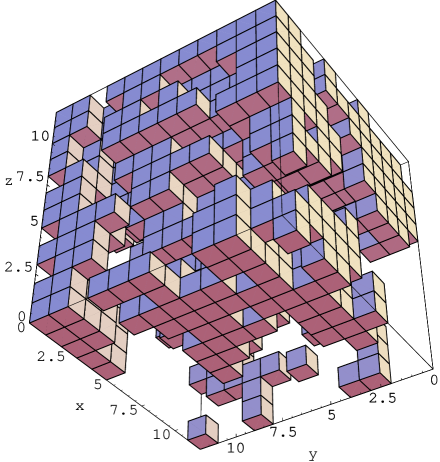
FIG. 8.: Difference of two projected TAP-like states ($L=12$ lattice).

The cluster is very space filling; to make this clear, we recommend looking at the display on a computer screen while it is being drawn (this gives far more information than the final printed picture where most of the cluster is hidden). Furthermore, the cluster is topologically non-trivial: one can guess at the numerous handles in its inside, and not surprisingly in our analysis it turns out to be sponge-like (it winds around the lattice in the three directions). One of the central questions for these types of objects concerns the scale beyond which (if any) they become homogeneous. This is a difficult question so it is wisest to focus on the cases for which $q$ is small: if any kind of homogeneity can be detected, it should be testable there.

As a probe of heterogeneities, we follow Houdayer et al. [18] and ask whether it is possible to push a needle all the way through the lattice without hitting the boundary of $G$ (the difference of the two projected TAP-like states). This has a direct and intuitive interpretation: let each site of $G$ be associated with a unit cube that is opaque, as displayed in the figure. We send light onto one face of the cube and ask whether $G$ stops all the light or whether some light is able to pass through the cube without being absorbed. If $G$ is homogeneous on all scales larger than the lattice spacing, the probability of absorbing all the light goes to $1$ as $L\to\infty$. Because of the up-down symmetry, we ask in fact whether both $G$ and its complement absorb all the light. We find, as in the $T=0$ landscape studies [18], that there is almost always a straight line parallel to a given axis that stays entirely in $G$ or entirely in its complement. The system is thus not opaque. We can extend this kind of study by generalizing the needle to a pencil or “tube”: now we try to draw not a single line, but $4$ parallel lines whose cross-section is a plaquette of our lattice (the basic square formed by $4$ bonds connecting nearest neighbors). The fatter the tube, the less likely it will be possible to slide it through without hitting the surface of $G$. To compare with the $T=0$ study, we have used the same cross-sections as there: tube “2” has the plaquette cross-section with $4$ sites; tube “3” has a diamond cross-section with $5$ sites, i.e., a central site and its $4$ nearest neighbors; finally tube “4” has for its cross section two adjacent plaquettes with a total of $6$ sites (the reader can find pictures of these cross-sections in Houdayer et al. [18].)

Table III gives the fraction of events for which there is at least one tube along the $x$ axis which “spans” the whole cube (i.e., is of length $L$) without touching the surface of $G$ (the tube sites are thus entirely in $G$ or in its complement). The data are for those disorder instances with at least two valleys and with the extra constraint that $0\leq q\leq 0.1$ where $q$ is the spin overlap of the projected TAP-like states.

TABLE III.: Fraction of events allowing a spanning tube through $G$ as a function of the tube cross-section type.

L	Tube “2”	Tube “3”	Tube “4”
6	0.44	0.18	0.09
8	0.49	0.13	0.20
12	0.46	0.19	0.16

These data are a bit too noisy to extract a reliable trend. At best, we can say that the data are compatible with increasing values of the spanning probabilities as $L$ grows; that is the behavior arising in the energy landscape study. This would mean that the difference of two projected TAP-like states is geometrically similar to the difference of two low-lying system-size excited states. These findings should be considered together with the evidence that the clusters are space-filling (see [15, 16]): a $2D$ plane will intersect the clusters with very high probability. Thus on scales comparable to $L$, the clusters are space filling, in agreement with the Parisi mean field theory.

VIII Discussion and conclusions

We believe that the analysis presented in this note sheds significant light on the issue of the behavior of finite dimensional, realistic spin glasses. On the one hand we stress the physical relevance of the picture of space filling sponges; on the other hand our numerical results from low $T$ Monte Carlo simulations give evidence for RSB with a mean field like scenario. Perhaps our most important point is that the results of low $T$ numerical simulations give the same indications as the ground state computations. This fact attenuates the long-standing doubt: “Are spin glass numerical simulations representative of low $T$ physics, or do they just contain artifacts due to the $T_{c}$ critical point?” Our answer is then that indeed recent numerical simulations do give information about the low $T$ physics. Similarly, ground state computations then characterize the low $T$ physics behavior of these systems.

A second important issue we address concerns entropic effects. We find that the mean field like features of the system arise with entropy and energy fluctuations; the mutual cancellation of these fluctuations allows the near degeneracy in the free-energy of different states. To see these fluctuations, it is necessary to introduce valleys that are in a sense the building blocks of what can be called finite volume equilibrium states.

A third point worth mentioning is that definitions such as sponge-like or droplet-like differences are very useful; not only do they seem more and more clear-cut as $L$ grows, but they also allow for a finer analysis. An illustration of this potential was given via a modified spin overlap (restricted to sponges) that appears to be more robust than the usual one. For the future, we expect these definitions to be extremely useful when trying to understand putative deviations of realistic spin glasses from the standard mean field picture.

There is a lot more that can be done; many issues should be understood in greater detail and checked on larger lattices (our largest size is $L=12$). Let us just give a bird’s-eye view of what we feel are some of the main questions. (1): All of our work was for a given temperature; the effect of raising and lowering the temperature should be investigated. (2): The study of the structure of valleys has only begun. Our focus here was on large and well separated valleys; clearly a complete picture requires one to consider the more general case. (3): We have analyzed the EA model with binary ($\pm$) couplings. For the lattice sizes we used, this discreteness showed up on the mean energy differences of valleys (see figure 5). Does this effect go away for large sizes and can one confirm numerically the expectation that the Gaussian couplings lead to similar results at large $L$?

Acknowledgments

We thank A. Billoire, J.-P. Bouchaud, E. Domany, J. Houdayer, F. Krzakala, M. Mézard and G. Parisi for very stimulating discussions. The LPTMS is an Unité de Recherche de l’Université Paris XI associée au CNRS. One of us (EM) warmly acknowledges the hospitality of the LPTMS during which part of this work was done. The numerical simulations were run on Kalix2, a Linux cluster located at the Physics Department of Cagliari University, and funded by MURST COFIN 1998 (Italy). FZ is supported by an EEC Marie Curie fellowship (contract HPMFCT-2000-00553).

Appendix

We want to characterize valleys or families of spin configurations by their local magnetizations, “à la TAP”, in analogy with what occurs in mean field models. However, from a thermodynamical point of view, it is not easy to define TAP states in a finite volume. Because of this, our definition of valleys is obtained by clustering according to the spin overlaps. One can consider the formal approach of clustering over all of configuration space where each configuration has a given probability, or one can use a more “hands-on” description, where one clusters equilibrium configurations (as obtained from our simulation). Since it is simpler to explain our clustering in the latter framework, we limit ourselves to that case here.

To cluster our configurations, we will use the mutual overlaps and a cut-off parameter $q^{*}$. To begin, we give two definitions. A valley is just a set of configurations; these will be selected by the clustering algorithm, but what matters is that for each valley $k$ one has a collection of configurations ${\cal C}_{n}^{k}$ ($n=1,...|V_{k}|$). Second, the TAP-like state associated with valley $k$ is the list of magnetizations $m_{i}^{(k)}\in[-1,1]$, one for each site $i$ of the lattice. By definition, we take $m_{i}^{(k)}$ to be the mean of $S_{i}$ when considering all the configurations belonging to valley $k$.

The logic of our approach can be summarized as follows: (i) a valley defines its TAP-like state; (ii) the TAP-like states tell us whether or not a new configuration should be assigned to one of the $k$ valleys. A sensible assignment rule is to impose that the overlap of this new configuration with the corresponding TAP-like state should be sufficiently large. In our algorithm, we first compute the spin overlaps between the new configuration and the $k$ TAP-like states; let $q^{(1)}$, $q^{(2)}$, … $q^{(k)}$ be these overlaps. The new configuration is then assigned to valley $j$ if $q^{(j)}$ is the largest of these overlaps and if $q^{(j)}\geq q^{*}$.

With these definitions, we can now explain our clustering procedure which is based on defining valleys and their TAP-like states self-consistently. Suppose we have built $k$ valleys so far; let their TAP-like states be ${\cal M}^{(1)}$, ${\cal M}^{(2)}$, …, ${\cal M}^{(k)}$. Suppose we want to increase $k$ by $1$. First, we initialize ${\cal M}^{(k+1)}$ by setting its $m_{i}^{(k+1)}$ to be equal to spin values $S_{i}$ of one of the configurations that is not assigned to any valley. Then we go through the rest of the un-assigned configurations, adding them successively to the pool defining the ($k+1$)th valley if their overlap $q^{(k+1)}$ with ${\cal M}^{(k+1)}$ is greater than $q^{*}$ (the overlap is defined in the usual way, $q=\sum_{1}^{N}S_{i}m_{i}/N$). Every time a configuration is added to the pool, we update ${\cal M}^{(k+1)}$ so that it always gives the average magnetization at each site for the configurations in valley $k+1$.

At the end of this pass, we have ${\cal M}^{(1)}$, ${\cal M}^{(2)}$, …, ${\cal M}^{(k+1)}$. But because ${\cal M}^{(k+1)}$ changes as one adds configurations to the pool, some of such configurations may see their overlap $q^{(k+1)}$ go below $q^{*}$. Furthermore, some of the configurations assigned to valleys $j$ ($j\leq k$) may end up being closer to ${\cal M}^{(k+1)}$ than to ${\cal M}^{(j)}$. It is thus necessary to rebuild all the valleys, so we first de-assign all the configurations and then we perform a new pass where a configuration is assigned to valley $r$ if both $q^{(r)}>q^{*}$ and $q^{(r)}>q^{(s)}$ for all $s\neq r$. After three iterations of this build/un-build process, our algorithm takes these to be the valleys and computes the corresponding ($k+1$) TAP-like states. These additional iterations improve the self-consistency and reduce the valleys’ dependencies on the ordering of the configurations. This procedure is very close in spirit to that given by Iba and Hukushima [22]; they also have TAP-like states and valleys that are defined self-consistently by an iterative algorithm.

The last issue pertinent to our method concerns the total number $M$ of valleys to be generated. In our implementation, we continue creating more valleys until either of the three following criteria are met: (1) all configurations are assigned to valleys; (2) one has reached the maximum number of valleys (set to $10$ in our code); (3) adding one more valley and its TAP-like state would lead to ($M+1$) TAP-like states whose cross-overlaps would not all be less than $q^{*}$. When that happens, we consider that a valley has been subdivided too far and we do not accept this ($M+1$)th TAP-like state.

REFERENCES

- [1] M. Mézard, G. Parisi, and M. A. Virasoro, Spin-Glass Theory and Beyond, Vol. 9 of Lecture Notes in Physics (World Scientific, Singapore, 1987).
- [2] Spin Glasses and Random Fields, edited by A. P. Young (World Scientific, Singapore, 1998).
- [3] G. Parisi, Phys. Lett. 73A, 203 (1979).
- [4] G. Parisi, Phys. Rev. Lett. 43, 1754 (1979).
- [5] G. Parisi, J. Phys. A Lett. 13, L115 (1980).
- [6] G. Parisi, J. Phys. A 13, 1101 (1980).
- [7] G. Parisi, J. Phys. A 13, 1887 (1980).
- [8] G. Parisi, Phys. Rev. Lett. 50, 1946 (1983).
- [9] A. J. Bray and M. A. Moore, in Heidelberg Colloquium on Glassy Dynamics, Vol. 275 of Lecture Notes in Physics, edited by J. L. van Hemmen and I. Morgenstern (Springer, Berlin, 1986), pp. 121–153.
- [10] D. S. Fisher and D. A. Huse, Phys. Rev. B 38, 386 (1988).
- [11] S. F. Edwards and P. W. Anderson, J. Phys. F 5, 965 (1975).
- [12] E. Marinari et al., J. Stat. Phys. 98, 973 (2000), cond-mat/9906076.
- [13] F. Krzakala and O. C. Martin, Phys. Rev. Lett. 85, 3013 (2000), cond-mat/0002055.
- [14] M. Palassini and A. P. Young, Phys. Rev. Lett. 85, 3017 (2000), cond-mat/0002134.
- [15] E. Marinari and G. Parisi, Phys. Rev. Lett. 85, 3332 (2000), cond-mat/0002457.
- [16] E. Marinari and G. Parisi, Phys. Rev. B 62, 11677 (2000), cond-mat/0005047.
- [17] G. Hed, A. Hartmann, D. Stauffer, and E. Domany, Phys. Rev. Lett. 86, 3148 (2001).
- [18] J. Houdayer, F. Krzakala, and O. C. Martin, Eur. Phys. J. B. 18, 467 (2000), cond-mat/0009382.
- [19] J. Houdayer and O. C. Martin, Europhys. Lett. 49, 794 (2000), cond-mat/9909203.
- [20] E. Marinari, in Advances in Computer Simulation, edited by J. Kertész and I. Kondor (Springer-Verlag, Berlin, 1988), p. 50.
- [21] G. Hed, A. Hartmann, and E. Domany, Europhys. Lett. 55, 112 (2001), cond-mat/0012451.
- [22] Y. Iba and K. Hukushima, Prog. Theo. Phys. Supp. 138, 462 (2000).
- [23] D. J. Thouless, P. W. Anderson, and R. G. Palmer, Phil. Mag. 35, 593 (1977).
- [24] E. Marinari and G. Parisi, Phys. Rev. Lett. 86, 3887 (2001).
- [25] H. G. Katzgraber, M. Palassini, and A. P. Young, Phys. Rev. B 63, 184422 (2001), cond-mat/0007113.