Active Membrane Fluctuations Studied by Micropipet Aspiration

Abstract

We present a detailed analysis of the micropipet experiments recently reported in J-B. Manneville et al., Phys. Rev. Lett. 82, 4356–4359 (1999), including a derivation of the expected behaviour of the membrane tension as a function of the areal strain in the case of an active membrane, i.e., containing a nonequilibrium noise source. We give a general expression, which takes into account the effect of active centers both directly on the membrane, and on the embedding fluid dynamics, keeping track of the coupling between the density of active centers and the membrane curvature. The data of the micropipet experiments are well reproduced by the new expressions. In particular, we show that a natural choice of the parameters quantifying the strength of the active noise explains both the large amplitude of the observed effects and its remarkable insensitivity to the active-center density in the investigated range.

87.22.Bt Membrane and subcellular physics and structure - 82.65.Dp Thermodynamics of surfaces and interfaces

I Introduction

Biological membranes are made up of a complex mixture of lipids and proteins. The lipid molecules form a bilayer structure which separates the cytoplasm of the cell from the outside. In addition to this structural role, the membrane also participates in a number of the living cell functions [1], mostly performed by proteins embedded inside the lipid bilayer, such as solute transport via ion channels or pumps, cell locomotion and adhesion, membrane transport through exocytic and endocytic pathways, signal transduction… Consequently, from the statistical physics point of view, biological membranes are strongly out of thermodynamic equilibrium, whereas most studies on membranes reported in the physics literature have been done at thermodynamic equilibrium [2]. In order to achieve a more complete physical description of biological membranes, this nonequilibrium aspect clearly has to be included. The field of membrane shape fluctuations is a good test case in which to examine the relevance of nonequilibrium effects. At thermodynamic equilibrium, the membrane shape fluctuates because of thermal noise, i.e., the Brownian motion of the bilayer. Such membrane will be called a ‘passive’ membrane in this paper. If a nonequilibrium noise source is superimposed to thermal noise, due for instance to the activity of membrane proteins, then the membrane is no longer at thermodynamic equilibrium. In that case, the membrane will be called ‘active’.

Recently, micropipet experiments on fluctuating giant vesicles containing bacteriorhodopsin (BR) reconstituted in the lipid bilayer have shown that the light-driven proton pumping activity of BR induces an amplification of the membrane shape fluctuations [3]. In these experiments, a larger excess area could be pulled out by micropipet aspiration when the proteins were activated. The results were qualitatively interpreted in terms of an increase of the effective membrane temperature and were not directly compared to theoretical predictions. In the present article, we give details about the experimental procedure (section II) and develop a theoretical framework to analyze quantitatively the micropipet experiments (sections III and IV). According to theory, a qualitatively new fluctuation spectrum is expected in the presence of a nonequilibrium noise source [4, 5, 6]. These earlier theories introduced the nonequilibrium activity in the membrane conformation equation only. This restrictive choice was made because the nonequilibrium force-density arising from the active proteins, when included in the Stokes equation for the solvent velocity field, altered the membrane fluctuation spectrum through terms which were subdominant at small wavenumber.

We show here that those nominally subdominant terms provide the most important contribution in the experimentally relevant range. This unexpected behavior is due to the very small value of the permeation coefficient. With this implementation, theory and experiment are brought in agreement (section IV). Even the absence of sensivity of the experimental data on the active center density appears as a natural consequence of the developed theory.

II Experimental procedure and results

A Bacteriorhodopsin

The bacteriorhodopsin (BR) is a $27\,$ kDa protein [7] purified from the so-called purple membrane of the halophilic bacteria Halobacterium salinarum [8]. Its structure is known at the atomic level with high resolution [9]. The BR absorption spectrum shows a maximum in the green-yellow wavelength around $566$ nm (Fig. 1).

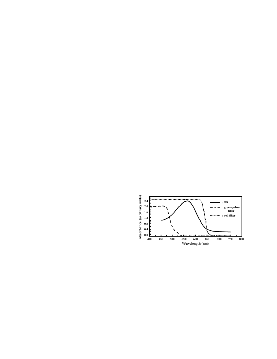
FIG. 1.: Absorption spectrum of the purple membrane suspensions used in the experiments (solid line) superimposed with the absorption spectra of the high-pass green-yellow filter (dashed line) and the high-pass red filter (dotted line).

When illuminated with green-yellow light, proton pumping is activated through a photocycle involving several distinct photointermediates [10]. The total duration of the photocycle is $\tau\simeq 5$ ms. Structural changes of the BR during the photocycle have been investigated to elucidate the translocation pathway of the proton across the protein. The pumping mechanism has been recently completely elucidated, so that BR is to date the best understood ion pump [11]. The proton pumping activity has been extensively studied in reconstituted systems, mostly in large unilamellar vesicles ($0.1-1\,\mathrm{\mu m}$ in diameter) [12].

B Giant vesicle formation

In reference [3], the electroformation technique of giant unilamellar vesicles ($10-100\,\mathrm{\mu m}$ in diameter) [13], modified according to [14] for BR incorporation in the lipid bilayer, was used to grow giant vesicles from a mixed lipid/protein dried film. The phospholipid EPC (Egg Phosphatidylcholine; Avanti Polar Lipids, Alabaster, Alabama, USA) is a mixture of lipids with different chain lengths and degrees of saturation and is known to be adequate for BR incorporation [15]. EPC ($0.5$ mg/ml) was first resuspended in diethyl ether. Concentrated BR ($18$ mg/ml) was then added at a molar ratio of $80$ lipid molecules per BR molecule. The mixture was sonicated at $0\,\mathrm{{}^{o}C}$ for $30$ seconds and a few microliters were deposited on ITO (Indium Tin Oxide) treated glass slides at $4\,\mathrm{{}^{o}C}$. The protein/lipid film was dried under vacuum overnight. A vesicle electroformation chamber was formed by assembling and sealing with wax (Sigillum wax; Vitrex, Copenhagen, Denmark) two ITO slides separated by $1$ mm Teflon spacers. The film was hydrated by injecting a $50$ mM sucrose solution in the chamber. An electric field ($1.5$ V AC) was applied across the chamber by connecting the ITO slides to copper electrodes. Giant vesicles were obtained in about two hours and transferred in a micromanipulation chamber filled with $50$ mM glucose to enhance the optical contrast between the inside and the outside of the vesicles. Sodium azide ($1$ mM) was first added to the sucrose and glucose solutions to avoid bacteria proliferation. In some experiments, respectively $16$ and $25\,\%$ (w/w) glycerol was added to both the internal and external solutions in order to increase the viscosity to respectively $1.5\eta_{w}$ and $2\eta_{w}$, where $\eta_{w}$ is the viscosity of water.

BR incorporation was checked by fluorescent labelling of BR with FITC (Fluorescein Isothiocyanate, F-143; Molecular Probes, Eugene, Oregon, USA) following a published protocol [16]. Excitation of the FITC was performed at $488$ nm with an argon laser (Spectra Physics, Les Ulis, France) through the epi-illumination pathway of an inverted microscope (Axiovert $135$; Zeiss, Oberkochen, Germany). The fluorescence images of the vesicles were acquired by a low light level SIT (Silicon Intensified Target) camera (LH4036; Lhesa, France) (see Fig. 2). The fluorescence intensity $I_{F}=(I_{ves}-I_{bgd})/I_{bgd}$, where $I_{ves}$ is the fluorescence intensity of the vesicle contour and $I_{bgd}$ is the background intensity, was measured by computer image analysis using a C++ custom software running on a Pentium 200-based computer with a Meteor frame grabber (Matrox, Rungis, France).

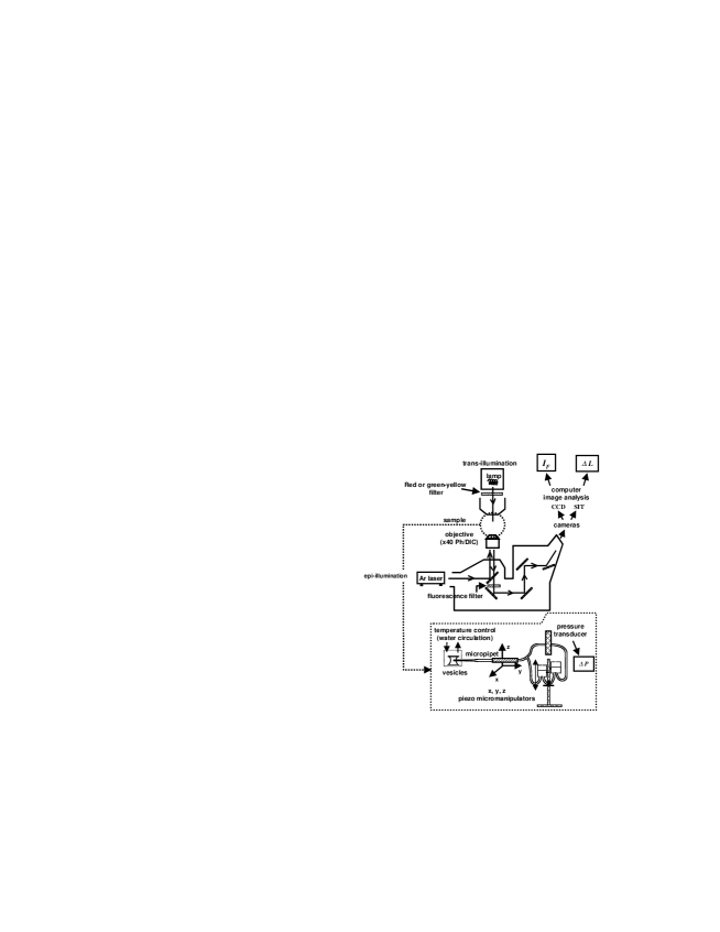
FIG. 2.: Experimental set-up designed for the micropipet experiments.

The BR was activated by illumination through a high-pass ($500$ nm) green-yellow filter located in the trans-illumination pathway (see Figs. 1 and 2), to avoid the non-pumping branched photocycle initiated if the M intermediate absorbs at $440$ nm [10]. To image the vesicles without activating the BR, a high-pass ($650$ nm) red filter was substituted for the green-yellow filter (see Figs. 1 and 2). The illumination power was in the same range as that known to fully activate BR reconstituted in large unilamellar vesicles ($10^{3}\,\mathrm{W/m^{2}}$) [12]. To correct for the different bandwidths of the green-yellow and red filters, the trans-illumination light focused on the specimen plane was adjusted to about $100\,\mathrm{mW/cm^{2}}$ in all the experiments. The sample was illuminated for at least $15$ minutes before starting an experiment, so that the BR was always in its light-adapted form [17].

It has been shown that the reverse phase evaporation technique used to incorporate BR in large unilamellar vesicles (typically $200$ nm in diameter) results in an asymmetrical orientation of the BR molecules across the lipid bilayer [12]. Consequently, for these vesicles, a proton gradient builds up across the lipid membrane upon activation, which inhibits BR pumping activity. However, since the electroformation technique is symmetrical, we do not expect any asymmetry in the BR orientation, and thus we do not expect inhibition of the pumping activity. To be on the safe side, we have performed additional experiments which were designed to cancel any proton gradient according to the following procedure. A classical way of suppressing the inhibitory proton gradient, without incorporating any additional active molecule in the membrane, is to add KCl (potassium chloride) to the solution, since protons can then codiffuse passively through the bilayer in the form of HCl, and since chloride ions can diffuse inside the vesicle to ensure electroneutrality. In reference [3], KCl was added to both the internal and external solutions up to $2$ mM, a concentration above which electroformation of giant vesicles fails, in order to get rid of a possible proton gradient. Our results proved to be insensitive to the addition of KCl .

C Micropipet experiments

The micropipet technique developed by Evans and coworkers [18] allows a quantification of the excess surface area stored in the membrane fluctuations by pulling it out with a micropipet aspiration: when a pressure difference is applied, the membrane is put under tension and sucked inside the pipet. The experimental set-up was built on an inverted microscope equipped with a $40$x objective (N.A. 0.75 air Ph2 Plan Neofluoar, Zeiss) for epi-fluorescence, phase contrast and differential interference contrast (DIC) microscopy. The transmission phase contrast or DIC images were recorded by a CCD (Charge Coupled Device) camera (Sony, Paris, France). The sample cell was temperature controlled at $15\,\mathrm{{}^{o}C}$ by a water flow to limit evaporation of the solution (see Fig. 2, bottom).

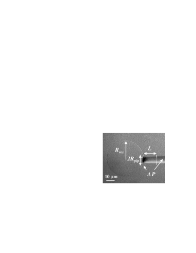
FIG. 3.: Typical micropipet experiment. The pressure difference $\Delta P$ is the difference between the pressure outside and inside the pipet. The intrusion length $L$ is the length of membrane aspirated inside the pipet when a pressure difference $\Delta P$ is applied. The bar represents $10\,\mathrm{\mu m}$.

Glass micropipets were pulled from $1$ mm outer diameter borosilicate capillaries (GC 100T-10; Phymep, Paris, France) with a micropipet-puller (P-97; Sutter Instruments Co., Novato, California, USA). The micropipet tip was cut on a microforge to obtain diameters up to $5-10\,\mathrm{\mu m}$. The pipets were treated with BSA (bovine serum albumin, $1\,\%$) for $30$ minutes to prevent adhesion of the lipid membrane to the glass pipet walls. A pipet holder was mounted on a three-dimensional piezo micromanipulator stage (Physik Instrumente, Waldbron, Germany) in order to control the position of the pipet tip within $0.1\,\mathrm{\mu m}$ accuracy. The pressure difference $\Delta P$ between the outside and the inside of the pipet was measured by a liquid-liquid pressure transducer (DP103-20; Validyne, SEI3D, France) with $0.01$ Pa accuracy. The pressure is imposed by a water height difference between two water filled tanks equipped with micrometric displacements (see Fig. 2, bottom). The absence of any air bubble in the water circuit running from the tanks to the micropipet is crucial and was checked before each experiment. The relationship between the pressure difference $\Delta P$ and the imposed membrane tension $\sigma$ directly derives from Laplace’s law [18]:

$$\sigma=\frac{R_{pip}}{2(1-R_{pip}/R_{ves})}\Delta P$$

where $R_{pip}$ is the pipet radius and $R_{ves}$ is the vesicle radius, both measured directly from the DIC image (see Fig. 3).

The excess area stored in the membrane shape fluctuations $\alpha$ is defined as $\alpha=(A-A_{p})/A$, where $A$ is the actual area of the fluctuating membrane and $A_{p}$ is the area projected on the mean plane of the membrane. During a micropipet experiment, the excess area decreases as the membrane undulations are pulled out by the increasing pressure difference. For a given $\Delta P$, an intrusion length $L$ is aspirated inside the pipet (see Fig. 3). A reference state $(\Delta P_{0},L_{0})$ is defined as the lowest suction pressure that can be applied in the experiment to aspirate the fluctuating vesicle inside the micropipet [18]. The variation of the excess area as compared to this reference state, the so-called areal strain $\Delta\alpha=\alpha_{0}-\alpha$, follows from geometrical considerations. To first order in $\Delta L=L-L_{0}$, we have [18]:

$$\Delta\alpha=\alpha_{0}-\alpha=\frac{(R_{pip}/R_{ves})^{2}-(R_{pip}/R_{ves})^{3}}{2R_{pip}}\Delta L$$

The increase of the intrusion length $\Delta L$ was measured by image analysis with pixel accuracy, i.e. $0.2\,\mathrm{\mu m}$ with the $40$x objective.

The excess area can be expressed using the local displacement $u$ of the membrane around its mean plane [19]:

$$\alpha=\langle(\nabla_{\perp}u)^{2}/2\rangle=\frac{1}{(2\pi)^{2}}\int_{0}^{q_{max}}\frac{1}{2}q_{\perp}^{2}\langle u({\bf q}_{\perp})^{2}\rangle 2\pi q_{\perp}dq_{\perp}$$ (1)

In the low q regime the convergence of the integral is guaranteed by a crossover from a curvature dominated regime $\langle u({\bf q_{\perp}})^{2}\rangle=kT/\kappa q_{\perp}^{4}$ to a tension dominated regime $\langle u({\bf q_{\perp}})^{2}\rangle=kT/\sigma q_{\perp}^{2}$ for a passive membrane, where $k$ is the Boltzmann constant, $T$ is the absolute temperature and $\kappa$ is the bending modulus of the membrane. The upper limit is $q_{max}=2\pi/a$, where $a$ is a microscopic length. In the entropic regime, i.e. at low tension, inserting the fluctuation spectrum of an equilibrium membrane gives the dependence of the excess area $\alpha$ as a function of the membrane tension $\sigma$ [18, 19]: $\alpha=(kT/8\pi\kappa)\ln(cst/\sigma)$, where $cst$ is an integration constant. The areal strain $\Delta\alpha=\alpha_{0}-\alpha$ is thus:

$$\Delta\alpha=\alpha_{0}-\alpha=\frac{kT}{8\pi\kappa}\ln\frac{\sigma}{\sigma_{0}}.$$ (2)

For a passive membrane, the linear relationship between the logarithm of the tension $\ln\sigma$ and the areal strain $\Delta\alpha$ allows the determination of the bending modulus $\kappa$. We will give in section IV a similar relation relevant to the active case.

D Essential results

The results reported in [3] and duplicated in Figure 4 show that when the vesicles are illuminated with green-yellow light, the slope of the logarithm of tension versus the areal strain is smaller than in the case where the vesicles are illuminated with red light. This indicates that the excess area is larger when the BR is illuminated with green-yellow light, and consequently that BR activity induces an amplification of the membrane shape fluctuations. The quality of the fit suggests that one can describe the effect of the BR activity in terms of an effective temperature $T^{eff}\simeq 2T$.

FIG. 4.: Variation of the logarithm of the tension $\sigma$ versus the areal strain $\Delta\alpha$ for the same vesicle containing BR, alternatively passive and active.

An other important feature of the experiment concerns the dependence of $T^{eff}$ on BR concentration. Fig. 5 shows that in a concentration range that we estimate between approximatively $10^{15}$ and $10^{16}\,\mathrm{BR/m^{2}}$ the effective temperature is essentially independent on BR concentration. This may look surprising since the BR activity is the driving force.

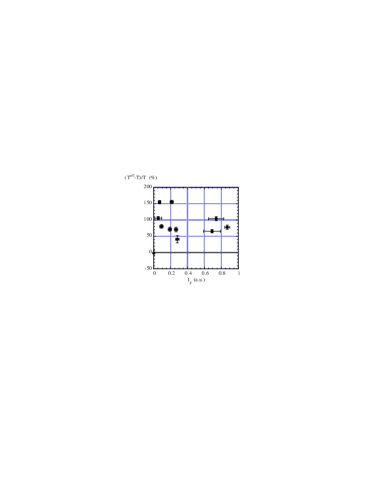
FIG. 5.: Variation of the effective temperature $T^{eff}$ of the active membrane as a function of the fluorescence intensity $I_{F}$, thus of the BR concentration.

Before developing the interpretation of these results, we must first guarantee their reliability, i.e. that it is an effect related to the out-of-equilibrium pumping activity of BR and nothing else. The control experiments with pure lipid vesicles obviously exclude a role of the lipids themselves. For these, we find for both green-yellow and red illumination the expected $kT/\kappa\simeq 0.1$ value [20]. Using simple estimates, we can also rule out the possibility of any thermally induced artefact due to the larger absorption of light by BR in the green-yellow wavelength. Assuming that one BR molecule absorbs one photon each $\tau\simeq 5$ ms, the total stationary flux (total energy received per unit area of membrane and per unit of time) is:

$$W=\frac{h\nu}{\tau}\times\bar{\rho}$$

where $h$ is the Planck constant, $\nu$ is the photon frequency and $\bar{\rho}$ is the mean BR density. In a pessimistic estimate, we assume that this total flux $W$ is dissipated via conduction in the surrounding water. The sample cell is temperature controlled by a cold water circulation and we assume that a temperature gradient arises from the BR heating between the membrane and the sample cell wall. This gradient extends over a typical length $L=1$ mm which is the size of the sample cell. With $C=4.18\times 10^{6}\,\mathrm{J.m^{-3}.\,{{}^{o}K}^{-1}}$ the heat capacity of water and $K_{T}=1.5\times 10^{-7}\,\mathrm{m^{2}/s}$ the heat diffusion coefficient, we have:

$$CK_{T}\frac{\Delta T}{L}=W=\frac{h\nu}{\tau}\times\bar{\rho}$$

and

$$\Delta T=\frac{h\nu}{\tau}\times\bar{\rho}\times\frac{L}{CK_{T}}$$

This yields a temperature increase of $\Delta T=2\times 10^{-3}\,\mathrm{{}^{o}K}$, five orders of magnitude smaller than the reported increase in effective temperature, which can not account for the observed effect [21]. Direct heating is just totally inefficient (note also that direct heating of water is clearly ruled out by the experiments on pure phospholipidic vesicles).

Most importantly, the experiments with glycerol prove that the observed effect is of nonequilibrium origin. The addition of glycerol modifies dynamic parameters such as the solvent viscosity $\eta$, the permeation coefficient $\lambda_{p}$ and the active force $F_{a}$. At thermodynamic equilibrium, such parameters cannot play a role in the fluctuation spectrum as imposed by the fluctuation-dissipation theorem. For an active membrane however, these parameters play a role as can be seen from references [4] or [6]. The addition of glycerol increases the solvent viscosity while it decreases its permeation coefficient. The results given in reference [3] report a lower increase in the effective temperature when $16\,\%$ and $25\,\%$ (w/w) glycerol is added, clearly revealing the out of equilibrium nature of the effect. This result is qualitatively consistent with the observation that the BR pumping activity is diminished upon addition of glycerol due to an increase in the lifetime of the M intermediate [22]. Finally, the fact that the observed effect does not depend on the measuring sequence (red light experiment or green light experiment first) rules out a potential role of the conformational change between the light-adapted and the dark-adapted states [17]. This is also consistent with the result that the ratio $kT/\kappa$ in the passive case is the same as that of the pure phospholipidic vesicles. The renormalisation of the bending rigidity by the BR is not measurable. All these observations give strong support to the assertion that the effect is indeed due to the proton pumping activity.

The use of an effective temperature to qualitatively interpret the results according to equation (2) is justified by the good quality of the linear fits of the micropipet experiments performed in [3]. However, we need to develop a complete theoretical analysis to understand all these experimental features quantitatively.

III Theory

As in references [4, 5, 6], we consider situations in which a membrane under tension is subjected to random forces of two different origins. These arise (i) from thermal agitation, i.e., the Brownian motion of the membrane, simply because membrane and solvent have a thermodynamic temperature, and (ii) from ‘biological’ activity such as proton pumping of the BR. The membrane equation of motion can be written to lowest order:

$$\lambda_{P}^{-1}(\frac{\partial u}{\partial t}({\bf r}_{\perp},t)-V_{z}({\bf r}_{\perp},t))=\delta P({\bf r}_{\perp},t)-\delta\Pi({\bf r}_{\perp},t)+F_{a}\psi({\bf r}_{\perp},t)+F_{a}^{\prime}\rho\Delta_{\perp}u({\bf r}_{\perp},t)+f_{p}({\bf r}_{\perp},t)$$ (3)

In this expression, $u({\bf r}_{\perp},t)$ is the membrane displacement at point ${\bf r}_{\perp}=(x,y)$ with respect to a $(x,y)$ reference plane orthogonal to ${\bf\hat{z}}$, the average membrane normal and $\Delta_{\perp}$ is the Laplacian in the $xy$ plane. $V_{z}({\bf r}_{\perp},t)$ is the fluid velocity, in the normal direction at the membrane surface; $\lambda_{P}$ is the membrane permeation coefficient. $\delta P({\bf r}_{\perp},t)=P({\bf r}_{\perp},z=0^{+},t)-P({\bf r}_{\perp},z=0^{-},t)$ is the pressure difference across the membrane and $\delta\Pi({\bf r}_{\perp},t)=\Pi({\bf r}_{\perp},z=0^{+},t)-\Pi({\bf r}_{\perp},z=0^{-},t)$ the osmotic pressure difference. This osmotic pressure difference results from the proton pumping activity: for each BR cycle one proton is transferred across the membrane. In principle the calculation of $\delta\Pi$ cannot be achieved without solving all dynamical equations of the problem. However, considering the convective term of the proton flux as a second order correction allows to evaluate $\delta\Pi$ separately. We postpone this derivation to appendix A. $f_{p}$ is the brownian noise acting on the membrane corresponding to the dissipation of energy in the permeation process and satisfies:

$$\langle f_{p}({\bf r}_{\perp},t)\rangle=0$$

$$\langle f_{p}({\bf r}_{\perp},t)f_{p}({\bf r}_{\perp}^{\prime},t^{\prime})\rangle=2kT\lambda_{P}^{-1}\delta({\bf r}_{\perp}-{\bf{r_{\perp}^{\prime}}})\delta(t-t^{\prime})$$

The term $F_{a}\psi({\bf r}_{\perp},t)$ results from the BR activity. More precisely $\psi({\bf r}_{\perp},t)=\rho^{\uparrow}({\bf r}_{\perp},t)-\rho^{\downarrow}({\bf r}_{\perp},t)$ is the local difference between the density $\rho^{\uparrow}({\bf r}_{\perp},t)$ of BR molecules transferring protons in the direction ${\bf\hat{z}}$ (up) and the density $\rho^{\downarrow}({\bf r}_{\perp},t)$ of BR molecules transfering protons in the -${\bf\hat{z}}$ direction (down). $F_{a}$ is the average elementary force transmitted to the membrane by a steady proton transfer. The flip-flop of BR is expected to be much slower than that of phospholipids and thus $\rho^{\uparrow}({\bf r}_{\perp},t)$ and $\rho^{\downarrow}({\bf r}_{\perp},t)$ can be considered as separately conserved quantities. As explained in section II, with our experimental conditions, the probability of inserting a BR molecule into the phospholipid membrane does not depend on the pumping direction, thus $\langle\rho^{\uparrow}\rangle=\langle\rho^{\downarrow}\rangle$ and $\langle\psi\rangle=0$. $\lambda_{P}F_{a}$ can be understood as measuring the average volume transferred through the membrane per BR and per unit time. Thus, $\lambda_{P}F_{a}\psi({\bf r}_{\perp},t)$, which we will refer to as the ‘active-permeative’ term, can also be understood as the local volume transferred through the membrane per unit area and per unit time due to the pumping imbalance between up and down BR molecules. Terms corresponding to the stochastic nature of the pumping activity have been omitted since they have been shown to lead to smaller effects than those due to the collective $\psi$ fluctuations [4, 5]. As discussed in [6], the fourth term describes the fact that pumping may work better when the membrane is curved with a given sign: $F_{a}^{\prime}$ measures this sensitivity per pump and $\rho=\rho^{\uparrow}({\bf r}_{\perp},t)+\rho^{\downarrow}({\bf r}_{\perp},t)$. There is experimental evidence for such a coupling in the functioning of certain ion-channels called TRAAK and TREK [23].

We further need equations for the fluid and for the BR density dynamics. Navier-Stokes equations have to be implemented in two ways: one first has to keep track of the Laplace force exerted by the membrane on the fluid, and this can be done in the usual way [5].

Secondly, each BR has a small but finite spatial extent. Its activity will disturb the ambient solvent in the form of a distribution of force densities in its vicinity. Since no external force source is present, the total force must vanish, but its first moment will in general be present. For convenience, we adopt the simplest set of force-densities consistent with this requirement: a pair of oppositely directed point forces, separated by a distance of order the size of a BR molecule. This implies a dipolar force density $F_{a}\left[\delta(z-w^{\uparrow})-\delta(z+w^{\downarrow})\right]\psi({\bf r}_{\perp},t)$ in the Stokes equations (this term will be called the ‘active-hydrodynamic’ term). $w^{\uparrow}$ and $w^{\downarrow}$ are lengths of the order of the BR size; their values are a priori unequal since the BR, or any molecule with unidirectional activity, is not up-down symmetric. Similarly, the term $F_{a}^{\prime}\left[\delta(z-w^{\uparrow})-\delta(z+w^{\downarrow}\right]\rho\Delta_{\perp}u({\bf r}_{\perp},t)$ describing the sensitivity of the force dipole to curvature should be kept. Thus, in the low Reynolds number regime appropriate to these experiments, we can write:

$$\begin{array}[]{rcl}0&=&-{\bf\nabla}P({\bf r},t)-\frac{\delta F}{\delta u}({\bf r}_{\perp},t)\delta(z){\bf\hat{z}}\\[6.0pt] &&\quad+F_{a}\left[\delta(z-w^{\uparrow})-\delta(z+w^{\downarrow})\right]\psi({\bf r},t){\bf\hat{z}}\\[6.0pt] &&\qquad+F_{a}^{\prime}\Delta_{\perp}u\left[\delta(z-w^{\uparrow})-\delta(z+w^{\downarrow})\right]\rho({\bf r}_{\perp},t){\bf\hat{z}}\\[6.0pt] &&\qquad+\eta\Delta{\bf V}({\bf r},t)+{\bf f}_{h}({\bf r},t),\end{array}$$ (4)

where ${\bf r}$ refers to the three-dimensional position vector, and ${\bf r}_{\perp}$ has the same meaning as in (3). $P({\bf r},t)$ is the three-dimensional pressure field, ${\bf V}({\bf r},t)$ the three-dimensional fluid velocity field, $F$ is the membrane free energy:

$$F=\frac{1}{2}\int d^{2}{\bf r}_{\perp}\left[\kappa(\Delta_{\perp}u({\bf r}_{\perp}))^{2}+\sigma({\bf\nabla}u({\bf r}_{\perp}))^{2}-2\Xi\psi({\bf r}_{\perp})\Delta_{\perp}u+\chi\psi^{2}({\bf r}_{\perp})\right]\$$

$\kappa$ is the membrane ‘bare’ bending modulus, $\sigma$ the membrane tension, $\Xi$ a coefficient linking membrane curvature and BR imbalance, $\chi$ the ‘bare’ susceptibility corresponding to that imbalance (for small enough densities $\chi\approx kT/\rho$). Orders of magnitude will be given in the next section. The third term of equation (4), is the ‘force dipole’ density already described, the fifth and sixth are the usual viscous terms and associated forces:

$\displaystyle\begin{array}[]{c}\langle{\bf f}_{h}({\bf r},t)\rangle=0\\[6.0pt] \langle{f_{hi}({\bf r},t)}{f_{hj}({\bf r^{\prime}},t^{\prime})}\rangle=2kT\eta\>\{-\delta_{ij}\nabla^{2}+\partial_{i}\partial_{j}\}\delta({\bf r}-{\bf r^{\prime}})\delta(t-t^{\prime})\end{array}$

Last, we need a dynamical equation for the BR imbalance density $\psi$. Following [6], we can write in the linear regime:

$$\frac{\partial\psi}{\partial t}=\Lambda\Delta_{\perp}\frac{\delta F}{\delta\psi}+\nabla_{\perp}\cdot{\bf f}_{\psi}$$ (5)

with $\Lambda=D/\chi$, where $D$ is the diffusion coefficient of the BR molecules in the membrane. This expression is valid for $\langle\psi\rangle=0$, in the absence of fluctuation corrections, and the last term of (5) is a conserving noise, i.e., the divergence of a random current with

$\displaystyle\begin{array}[]{c}\langle{\bf f}_{\psi}({\bf r_{\perp}},t)\rangle=0\\[6.0pt] \langle f_{\psi i}({\bf r_{\perp}},t)f_{\psi j}({\bf r_{\perp}}^{\prime},t^{\prime})\rangle=2\Lambda kT\delta_{ij}\>\delta({\bf r_{\perp}}-{\bf r_{\perp}^{\prime}})\delta(t-t^{\prime})\end{array}$

In order to compare experiment and theory, we need to calculate the equal time correlation function $\langle u({\bf q}_{\perp},t)u({\bf q}_{\perp}^{\prime},t)\rangle$. We first eliminate $V_{z}$ in (3) by solving for it from the Stokes equation (4) in Fourier space to get:

$$\frac{\partial u}{\partial t}({\bf q}_{\perp},t)+\tau_{u}^{-1}u({\bf q}_{\perp},t)=\beta\>\psi({\bf q}_{\perp},t)+\mu$$ (6)

$$\frac{\partial\psi}{\partial t}({\bf q}_{\perp},t)+\tau_{\psi}^{-1}\psi({\bf q}_{\perp},t)=\gamma\>u({\bf q}_{\perp},t)+\nu$$ (7)

in which we have chosen the convention

$\displaystyle f({\bf q}_{\perp},t)=\int f({\bf r}_{\perp},t)\>\exp(i{\bf q}_{\perp}\cdot{\bf r}_{\perp})\,d^{2}{\bf r}_{\perp}$

for Fourier transforms, and used $\delta\Pi\simeq 2kT\dot{a}\psi({\bf q}_{\perp},t)/D_{P}q_{\perp}$ where $\dot{a}$ is the proton pumping rate and $D_{P}$ an effective proton diffusion coefficient (see appendix A). The parameters entering equations (6) and (7) are listed below:

$\displaystyle\begin{array}[]{lr}\tau_{u}^{-1}=(\lambda_{P}+\frac{1}{4\eta q_{\perp}})(\sigma q_{\perp}^{2}+\kappa q_{\perp}^{4})+\rho\lambda_{P}F_{a}^{\prime}q_{\perp}^{2}-\frac{\rho{\mathcal{P}}_{a}^{\prime}w}{4\eta}q_{\perp}^{3}&\\[6.0pt] \tau_{\psi}^{-1}=\Lambda\chi q_{\perp}^{2}=Dq_{\perp}^{2}&\qquad\bar{F_{a}}=F_{a}-2kT\dot{a}/D_{P}q_{\perp}\\[6.0pt] \beta=\lambda_{P}\bar{F_{a}}-{\mathcal{P}}_{a}\frac{q_{\perp}w}{4\eta}-\Xi q_{\perp}^{2}(\lambda_{P}+\frac{1}{4\eta q_{\perp}})&\qquad{\mathcal{P}}_{a}=F_{a}\frac{w_{\uparrow}^{2}-w_{\downarrow}^{2}}{2w}\\[6.0pt] \mu=\lambda_{P}f_{p}({\bf q}_{\perp},t)+\frac{1}{2\pi\eta}\int\frac{{\bf f}_{h}({\bf q},t)\cdot{\bf\hat{z}}}{q^{2}}dq_{z}&\qquad{\mathcal{P}}_{a}^{\prime}=F_{a}^{\prime}\frac{w_{\uparrow}^{2}-w_{\downarrow}^{2}}{2w}\\ \gamma=-\Lambda\Xi q_{\perp}^{4}&\\ \nu=-i{\bf q}_{\perp}\>{\bf f}_{\psi}({\bf q}_{\perp},t)&\end{array}$

Calculating the equal time $\langle u({\bf q}_{\perp},t)u({\bf q}_{\perp}^{\prime},t)\rangle$ correlation function is straightforward although somewhat tedious; we find

$$\langle u({\bf q}_{\perp},t)u(-{\bf q}_{\perp},t)\rangle=\frac{kT}{(\tau_{u}^{-1}+\tau_{\psi}^{-1})({\tau_{u}^{e}}^{-1}+\tau_{a}^{-1})}\left[\frac{(\lambda_{P}F_{a}-{\mathcal{P}}_{a}\frac{q_{\perp}w}{4\eta})^{2}}{\chi}+(\tau_{u}^{-1}+\tau_{\psi}^{-1}+\tau_{a}^{-1})(\lambda_{P}+\frac{1}{4\eta q_{\perp}})\right]$$ (8)

with

$$\tau_{a}^{-1}=\frac{\Xi}{\chi}\>q_{\perp}^{2}\>\left(\lambda_{P}F_{a}-{\mathcal{P}}_{a}\frac{q_{\perp}w}{4\eta}\right)$$

${\tau_{u}^{e}}^{-1}$ has exactly the same structure than $\tau_{u}^{-1}$, but $\kappa$ is replaced by $\kappa^{e}=\kappa-\Xi^{2}/\chi$. Note that in the absence of active noise, (8) reduces to its thermal equilibrium expression, as it should.

In the long wavelength limit, one finds for a membrane under tension (neglecting the osmotic contribution):

$$\langle u({\bf q}_{\perp},t)u(-{\bf q}_{\perp},t)\rangle=\frac{kT^{e}}{\sigma q_{\perp}^{2}}$$ (9)

with $T^{e}=T\;(1+16\lambda_{P}^{2}F_{a}^{2}\eta^{2}/\chi\sigma)$ which means that a tense membrane is flat at longwavelength, even in the presence of non-thermal noise, and that one can define an effective temperature higher than the actual one.

For a tensionless membrane, we now find for $q_{\perp}\rightarrow 0$:

$$\langle u({\bf q}_{\perp},t)u(-{\bf q}_{\perp},t)\rangle=\frac{k{T^{\prime}}^{e}}{\kappa q_{\perp}^{4}}$$ (10)

with ${T^{\prime}}^{e}=T\cdot(\lambda_{P}F_{a})^{2}\kappa/[\chi(D+\rho\lambda_{P}F_{a}^{\prime})(\rho\lambda_{P}F_{a}^{\prime}+\frac{\Xi}{\chi}\lambda_{P}F_{a})]$. This expression is equivalent to the one given in [6], and in particular the effective temperature does not depend on the pumping density for small enough densities. At long enough wavelength, the osmotic term should always dominate, but we show in the next section that the experimentally relevant regimes in fact imply the contribution of the force dipoles.

IV Experimentally relevant regime and discussion

Let us first point out that in all equations the active-permeative and the active-hydrodynamic terms come in the combination:

$\displaystyle\lambda_{P}F_{a}-\frac{{\mathcal{P}}_{a}}{4\eta}{q_{\perp}w}$

This tells us that in the long wavelength limit, the active-permeative term always dominates over the active-hydrodynamic term. However, the crossover wavevector, below which the active-permeative term wins reads:

$\displaystyle q_{\perp c}=\frac{4(\eta\lambda_{P})F_{a}}{w{\mathcal{P}}_{a}}$

or for the corresponding length:

$\displaystyle l_{\perp c}=2\pi\frac{w}{4\eta\lambda_{P}}\cdot(\frac{{\mathcal{P}}_{a}}{F_{a}})$

That is with $\eta\lambda_{P}=l_{P}$ the permeation length, and ${\mathcal{P}}_{a}/{F_{a}}\simeq w$:

$$l_{\perp c}\simeq 2\pi\frac{w^{2}}{4l_{P}}$$

At first sight, one might be tempted to state that this crossover length is microscopic, but it turns out that $l_{P}$ is of the order of, or smaller than, a Fermi. Indeed, with $\eta=10^{-3}$ kg/m.s and $\lambda_{P}\lesssim 10^{-12}\,\mathrm{m^{3}/N.s}$ [24] , we find $l_{P}\lesssim 10^{-15}$ m. Then, with $w\simeq 5\cdot 10^{-9}$ m, we find:

$$l_{\perp c}\simeq 3\cdot 10^{-2}\,\mathrm{m}$$

As a result, all active-permeation terms may be omitted in the micron and submicron length scales we are dealing with ($2\pi/R_{ves}\simeq 3\cdot 10^{5}\,{\mathrm{m}}^{-}1\lesssim q\lesssim 2\pi/a\simeq 6\cdot 10^{10}\,{\mathrm{m}}^{-}1$, with $R_{ves}\simeq 20\,\mathrm{\mu m}$ and $a\simeq 0.1\,$ nm).

The osmotic contribution is negligible as well. To see this, compare $2\lambda_{P}kT\dot{a}/D_{P}q_{\perp}$ and ${\mathcal{P}}_{a}q_{\perp}w/4\eta$: this yields the cross over wavevector

$$q_{\perp c}^{\prime}=\left(\frac{8\lambda_{P}\eta kT\dot{a}}{{\mathcal{P}}_{a}wD_{P}}\right)^{1/2}$$

or the cross over length

$$l_{\perp c}^{\prime}=2\pi\left(\frac{{\mathcal{P}}_{a}wD_{P}}{8\lambda_{P}\eta kT\dot{a}}\right)^{1/2}$$

With an effective proton diffusivity $D_{P}\simeq 10^{-9}\,\mathrm{m^{2}/s}$, a pumping rate $\dot{a}=10^{3}\,\mathrm{s^{-1}}$, ${\mathcal{P}}_{a}\simeq\kappa\simeq 10kT$ (see appendix B), and other material parameters as above, one finds $l_{\perp c}^{\prime}\simeq 10^{-2}$ m: the osmotic contribution is totally negligible as well. In the case of ion channels for which $\dot{a}=10^{7}\,\mathrm{s^{-1}}$, the cross over length is reduced by a factor hundred, that is to a few tens of microns; this may be accessible to experiment. Similarly, since $\l_{P}\ll q^{-1}$, terms arising from permeative friction may entirely be omitted in the equations. We have now:

$\displaystyle\begin{array}[]{lr}\tau_{u}^{-1}=\frac{1}{4\eta}(\sigma q_{\perp}+\tilde{\kappa}q_{\perp}^{3})&\qquad\text{with}\>\tilde{\kappa}=\kappa-\rho{\mathcal{P}}_{a}^{\prime}w\\[6.0pt] {\tau_{u}^{e}}^{-1}=\frac{1}{4\eta}(\sigma q_{\perp}+\tilde{\kappa^{e}}q_{\perp}^{3})&\qquad\quad\tilde{\kappa^{e}}=\kappa^{e}-\rho{\mathcal{P}}_{a}^{\prime}w\\[6.0pt] \tau_{\psi}^{-1}=Dq_{\perp}^{2}&\\[6.0pt] \tau_{a}^{-1}=-\frac{\Xi}{4\chi\eta}{\mathcal{P}}_{a}wq_{\perp}^{3}&\\ \end{array}$

A further simplification can be obtained with the remark that in our experimental conditions $D\ll{(\sigma\kappa)}^{1/2}\eta^{-1}$ (i.e., more precisely, $D\lesssim 10^{-2}{(\sigma\kappa)}^{1/2}\eta^{-1}$ with $D\simeq 10^{-12}\,\mathrm{m^{2}/s}$ [25]). This means that one can further ignore the diffusion term in the $\langle u({\bf q}_{\perp},t)u(-{\bf q}_{\perp},t)\rangle$ correlation function. Under such conditions, equation (8) reduces to the expression:

$$\langle u({\bf q}_{\perp},t)u(-{\bf q}_{\perp},t)\rangle\simeq\frac{kT}{\sigma q_{\perp}^{2}+\tilde{\tilde{\kappa^{e}}}q_{\perp}^{4}}+\frac{kT\left[{\mathcal{P}}_{a}^{2}w^{2}-\Xi{\mathcal{P}}_{a}w\right]}{\chi(\sigma+\tilde{\kappa}q_{\perp}^{2})(\sigma+\tilde{\tilde{\kappa^{e}}}q_{\perp}^{2})}$$ (11)

where $\tilde{\tilde{\kappa^{e}}}=\tilde{\kappa^{e}}-{\mathcal{P}}_{a}w\Xi/\chi$
From this correlation function, we can calculate the relationship between the areal strain and the membrane tension:

$$\Delta\alpha=\alpha_{0}-\alpha=\frac{kT}{8\pi}\left(\frac{{\mathcal{P}}_{a}^{2}w^{2}-\Xi{\mathcal{P}}_{a}w}{\tilde{\tilde{\kappa^{e}}}\tilde{\kappa}\chi}+\frac{1}{\tilde{\tilde{\kappa^{e}}}}\right)\ln\left(\frac{\sigma}{\sigma_{0}}\right)$$ (12)

or

$$\Delta\alpha=\alpha_{0}-\alpha=\frac{kT^{eff}}{8\pi\kappa}\ln(\frac{\sigma}{\sigma_{0}})$$ (13)

with

$$\frac{T^{eff}}{T}=\frac{\kappa}{\tilde{\tilde{\kappa^{e}}}}\left(1+\frac{{\mathcal{P}}_{a}^{2}w^{2}-\Xi{\mathcal{P}}_{a}w}{\tilde{\kappa}\chi}\right)$$ (14)

The functional relation (13) is identical to the one holding in the equilibrium case (except that the ‘temperature’ is an effective nonequilibrium noise level) and is clearly compatible with the experimental results. The whole theory accounts well for the experimental observations if we note in addition the following four results:

• the value of the bending modulus, measured in the passive case, is insensitive to the BR concentration and equal to that of pure phospholipidic membrane,

• the effective temperature is about twice as large as the actual temperature,

• the effective temperature is essentially independent of the BR surface concentration in the investigated domain,

• the reduced effective temperature difference $(T^{eff}-T)/T$ decreases by a factor 3 when 25 $\%$ glycerol is added.

The first observation is easily explained, as detailed in appendix B. In order to discuss the second and third observations one must estimate the different terms entering equation (14). We provide details on these estimates in appendix B. We expect:

$\displaystyle\begin{array}[]{c}|{\mathcal{P}}_{a}|\simeq\kappa\\[6.0pt] |\Xi|\simeq wkT\\[6.0pt] |{\mathcal{P}}_{a}^{\prime}|\simeq\kappa w\\[6.0pt] \chi\simeq kT/\rho\simeq kTl^{2}\end{array}$

where $l$ is the average distance between BR molecules. We have been able to vary the concentration $\rho$ over approximately one order of magnitude, that is roughly $l$ from $w$ to $3w$. With such estimates, and chosing the signs in such a way that the system is stable, we expect:

$$\frac{T^{eff}}{T}\simeq\frac{1+\left(\frac{\kappa}{kT}+2\right)\frac{w^{2}}{l^{2}}}{\left(1+\frac{w^{2}}{l^{2}}\right)\left(1+\left(2-\frac{kT}{\kappa}\right)\frac{w^{2}}{l^{2}}\right)}$$

with $0.3\leq w/l\leq 1$ and knowing that $\kappa\simeq 10kT$, we find:

$$1.7\lesssim\frac{T^{eff}}{T}\lesssim 2.3$$

which is in very reasonable agreement with experiment. Of course, the numbers chosen above have some degree of arbitrariness, but one can change them appreciably while retaining a ratio $T^{eff}/T$ of order 2. For instance, $\Xi$ may be set to zero, keeping other values unchanged, and one finds $2<T^{eff}/T<2.7$, which is less satisfactory but not off scale.

Let us now turn to the glycerol dependence. It has been measured that a 25 $\%$ glycerol addition to water reduces the pumping activity of the bacteriorhodopsin by a factor $2.5$ [22]. It is thus clear that both ${\mathcal{P}}_{a}$ and ${\mathcal{P}}_{a}^{\prime}$ (and perhaps $\Xi$) have to be reduced by a factor $2.5$; all other parameters are essentially unchanged, as shown by the experiments performed with red light. The same type of estimate as before give the expected reduction of $(T^{eff}-T)/T$ by a factor three.

The net conclusion is thus that our analysis provides a satisfactory account of the experiment, although it is not able to pinpoint accurately values for $\Xi$, ${\mathcal{P}}_{a}^{\prime}$ and ${\mathcal{P}}_{a}$. A more accurate experiment should reveal that the effective temperature should depend on BR density in a non trivial way. At low density, the effective temperature should be essentially equal to the actual temperature; it should increase proportionally to the density at moderate densities; eventually, at larger densities, it could even decrease after going through a maximum. Together with an independent measurement of $\chi$, it should allow us to measure at least ${\mathcal{P}}_{a}$ and ${\mathcal{P}}_{a}^{\prime}$. Our current accuracy does not allow for such a detailed analysis.

Thus, the proposed analysis gives a natural interpretation of the experimental data. It is one of those intriguing cases in which terms nominally subdominant in wavenumber provide by far the leading contribution. This pecularity is due to the very small value of the permeation coefficient: in the experimentally accessible domain, the membrane is practically impermeable and the effects due directly to the force exerted by the active centers on the membrane are negligible.

A Osmotic pressure difference

Since BR selectively pumps protons, we just have to consider the osmotic pressure resulting from the three dimensional proton density $n({\bf r},t)$:

$$\Pi=kTn({\bf r},t)$$ (A1)

The protons dynamics is described as usual by conservation equations in each half space, above and below the membrane:

$$\frac{\partial n}{\partial t}({\bf r},t)+{\bf\nabla}\cdot{\bf J}_{n}=0$$ (A2)

$${\bf J}_{n}=n{\bf V}-D_{P}{\bf\nabla}n$$

At the membrane, the coarsegrained proton flux ${\bf J}_{n}\cdot{\bf\hat{z}}$ in the membrane normal direction ${\bf\hat{z}}$, is given by the BR active transport:

$${\bf J}_{n}\cdot{\bf\hat{z}}=\psi({\bf r},t)\>\dot{a}$$

where $\dot{a}$ is the pumping rate, and $\psi({\bf r},t)$ is defined in the main text. For a macroscopically symmetric membrane, $\psi$, $n$ and ${\bf V}$ are ‘small’ fluctuating quantities. So the convective term can be omitted, as a second order correction. Now to the linear order, equation (A2) becomes in ‘hybrid’ Fourier space (with obvious notations):

$$\begin{array}[]{c}i\omega n(z,{\bf q}_{\perp},\omega)+D_{P}q_{\perp}^{2}n(z,{\bf q}_{\perp},\omega)-D_{P}\frac{\partial^{2}}{{\partial z}^{2}}n(z,{\bf q}_{\perp},\omega)=0\\[6.0pt] -D_{P}\frac{\partial n}{\partial z}(z=0^{+},{\bf q}_{\perp},\omega)=-D_{P}\frac{\partial n}{\partial z}(z=0^{-},{\bf q}_{\perp},\omega)=\psi({\bf q}_{\perp},\omega)\dot{a}\end{array}$$ (A3)

The solution to this problem is straightforward. One finds:

$$n(z=0^{+},{\bf q}_{\perp},\omega)-n(z=0^{-},{\bf q}_{\perp},\omega)=\frac{2\psi({\bf q}_{\perp},\omega)\dot{a}}{D_{P}(i\frac{\omega}{D_{P}}+q_{\perp}^{2})^{1/2}}$$

so that

$$\delta\Pi({\bf q}_{\perp},\omega)=\frac{2kT\psi({\bf q}_{\perp},\omega)\dot{a}}{D_{P}{(\frac{i\omega}{D_{P}}+q_{\perp}^{2})}^{1/2}}$$ (A4)

The typical frequency over which $\psi({\bf q}_{\perp},\omega)$ varies is $Dq_{\perp}^{2}$. Eventhough $D_{P}$ is an effective diffusion coefficient renormalized by the time the proton spends attached to the hydrazoic acid resulting from the conversion of sodium azide in solution [26], one always has $D_{P}\gg D$, and thus the term $\omega/D_{P}$ may be safely omitted in equation (A4). Then, one can equivalently write:

$$\delta\Pi({\bf q}_{\perp},\omega)\simeq\frac{2kT\psi({\bf q}_{\perp},\omega)\dot{a}}{D_{P}q_{\perp}}$$ (A5)

B Orders of magnitude of the theoretical parameters

The long wavelength effective membrane curvature modulus $\kappa^{e}$, is as shown in section III:

$$\kappa^{e}=\kappa-\frac{\Xi^{2}}{\chi}$$ (B1)

It is easy to convince oneself that the coupling term $\Xi$ in fact depends on the pumping activity. Let us first consider the passive case, and call the corresponding coeffiecient $\Xi_{p}$. A BR molecule with a given orientation may ’prefer’ a given curvature sign for several different reasons. The first and most obvious one is linked to a putative wedge shape. In such a case, one expects:

$$\Xi_{p}\simeq\kappa R\theta$$

in which $R$ is the ’radius’ of the BR molecule and $\theta$ the wedge angle. The experiments performed with red light tell us:

$$\frac{\Xi_{p}^{2}}{\chi}\ll\kappa$$

That is:

$$\theta^{2}\ll\frac{kT}{\kappa}\left({\frac{l}{R}}\right)^{2}$$

At the highest densities $l\simeq w\simeq R$, so with $\kappa=10kT$ the experiment requires $\theta\ll 1/3$, which is obviously a ‘weak’ requirement: the absence of up-down symmetry in BR requires the existence of a wedge, but inspection of the molecular structure suggests that it is very small (for instance, it is very hard to coin a sign to it). So, the ‘steric’ contribution to $\Xi_{p}$ can be safely neglected.

There can however, be other contributions and the next most obvious one results from flexoelectricity: a curved membrane generates an electric polarisation, hence a transmembrane electric field. Again, the absence of up-down symmetry in BR tells us that it must have a non zero electric dipole. The energy of the dipole in this transmembrane field, provides the coupling between curvature and $\psi$. With the usual definitions, the transmembrane electric field can be written:

$$E=-\frac{e}{\epsilon w}\Delta_{\perp}u$$ (B2)

in which $\epsilon$ is the dielectric permittivity of the hydrophobic layer and $e$ is the flexoelectric coefficient discussed by Petrov for instance [27]. If we call $p$ the BR average longitudinal dipole, one has:

$$\Xi_{p}^{f}=\frac{ep}{\epsilon w}$$

The flexoelectric coefficient $e$ is a measured quantity [27]:

$$|e|\simeq 1.3\cdot 10^{-20}\;\mathrm{C}$$

Estimating $p\simeq\text{a few}\,q\cdot\delta$, in which $q$ is a unit charge and $\delta$ a distance of the order of a fraction of the membrane thickness, e.g. the hydrophilic part (note that it cannot be much larger otherwise the BR would not be membrane soluble), and taking the dielectric permittivity of the hydrophobic layer of the order of $\epsilon\simeq 3\,\epsilon_{0}$, with the dielectric permittivity of vacuum $\epsilon_{0}\simeq 8.8\cdot 10^{-12}\,\mathrm{F.m^{-1}}$, we find:

$$\frac{\Xi_{p}^{f\,2}}{\kappa\chi}<10^{-2}$$

So in this case as well, one does find $\kappa^{eff}\simeq\kappa$.

When the BR undergoes its pumping activity, the flexoelectric energy is dominated by the time average energy of the proton in the flexoelectric potential $e\Delta_{\perp}u/\epsilon$; assuming a duty ratio of one tenth, we expect then:

$$\Xi_{a}^{f}\simeq\frac{qe}{10\cdot\epsilon}\simeq\frac{1}{100\cdot\epsilon}q^{2}\simeq w\;kT$$

The force dipole ${\mathcal{P}}_{a}$ has the dimensions of an energy, and hence must be a fraction of the green-yellow photon energy. As a rough rule of thumb, we take again a duty ratio of a tenth:

$${\mathcal{P}}_{a}\simeq\frac{h\nu}{10}\simeq\kappa$$

The curvature dependence of the force dipole can be estimated in a way similar to that used for $\Xi$. During its pumping cycle, the BR/proton system has probably to overcome a potential barrier $W_{b}$. The pumping rate is then controled by a Boltzmann factor $\exp(-W_{b}/kT)$. In the presence of curvature, the barrier is modified by the energy of the proton in the flexoelectric potential at the barrier location. We call $xW_{b}$ this location. Thus, the activity is multiplied by a factor $\exp\left[-x(eq\Delta_{\perp}u)/(\epsilon\cdot kT)\right]$ which can be linearized for small curvatures. Hence, we expect (with $x$ of the order of a few tenths):

$${\mathcal{P}}_{a}^{\prime}\simeq-{\mathcal{P}}_{a}x\frac{eq}{\epsilon\cdot kT}\simeq-\,\text{a few}\,w\cdot\kappa$$

Note that one could in principle estimate this coefficient by measuring the pumping activity in liposomes, as a function of liposome radius: the net result would strongly depend on the value of $x$. For $x\simeq$ a few tenths, one would need % accuracy to measure the curvature dependence. For $x\simeq 1$, the effects would be much larger and the exponential nature of the relation should start to show up. However, even if the direct effect is not easily measurable, the incidence on formula (14) can be important.

REFERENCES

- [1] See for instance, Molecular Biology of the Cell, Ch. 10 (Third Ed.) by B. Alberts et al. (Garland Publishing, New York, 1994).
- [2] Structure and Dynamics of Membranes, edited by R. Lipowsky, E. Sackmann (Elsevier North Holland, Amsterdam, 1995); M. Bloom, E. Evans, and O. G. Mouritsen, Q. Rev. Biophys. 24, 293–297 (1991) and references therein; R. Lipowsky, Nature 349, 475–481 (1991) and references therein.
- [3] J-B. Manneville, P. Bassereau, D. Lévy, and J. Prost, Phys. Rev. Lett. 82, 4356–4359 (1999).
- [4] J. Prost and R. Bruinsma, Europhys. Lett. 33, 321–326 (1996).
- [5] J. Prost, J-B. Manneville, and R. Bruinsma, Eur. Phys. J. B 1, 465–481 (1998).
- [6] S. Ramaswamy, J. Toner, and J. Prost, Pramana-J. Phys. 53, 237–242 (1999); S. Ramaswamy, J. Toner, and J. Prost, Phys. Rev. Lett. 84, 3494–3497 (2000).
- [7] R. Henderson and P. N. T. Unwin, Nature 257, 28–32 (1975).
- [8] D. Oesterhelt and W. Stoeckenius, Methods Enzymol. 31, 667–678 (1974).
- [9] Y. Kimura et al., Nature 389, 206–211 (1997) ; E. Pebay-Peyroula et al., Science 277, 1676–1681 (1997).
- [10] For recent reviews see: U. Haupts, J. Tittor and D. Oesterhelt, Ann. Rev. Biophys. Biomol. Struct. 28, 367–399 (1999); S. Subramaniam et al., J. Mol. Biol. 287, 145–161 (1999); J. K. Lanyi, J. Biol. Chem. 272, 31209–31212 (1997); W. Kuhlbrandt, Nature 406 569–570 (2000); J. Heberle et al., Biophys. Chem. 85 229–248 (2000); N.A. Dencher et al. Biochim. Biophys. Acta 1460 192–203 (2000).
- [11] See for example: H. Luecke et al., Science 286, 255–260 (1999); H. Luecke, H.-T. Richter, and J. K. Lanyi, Science 280, 1934–1937 (1998); S. Subramaniam, and R. Henderson Nature 406 653–657 (2000); H.J. Sass et al. Nature 406 649–653 (2000); A. Royant et al. Nature 406 645–648 (2000).
- [12] M. Seigneuret and J-L. Rigaud, FEBS Lett. 228, 79–84 (1988); M. Seigneuret and J-L. Rigaud, Biochemistry 25, 6723–6730 (1986); J.-L. Rigaud, A. Bluzat, and S. Büschlen, Biochem. Biophys. Res. Commun. 111, 373–382 (1983).
- [13] M. I. Angelova et al., Prog. Coll. Polym. Science 89, 127–131 (1992).
- [14] D. Lévy, personnal communication.
- [15] F. Dumas et al., Biophys. J. 73, 1940–1953 (1997).
- [16] J. Heberle and N. A. Dencher, Proc. Nat. Acad. Sci. USA 89, 5996-6000 (1992).
- [17] T. Kouyama, R. A. Bogomolni, and W. Stoeckenius, Biophys. J. 48, 201–208 (1985).
- [18] E. Evans and W. Rawicz, Phys. Rev. Lett. 64, 2094–2097 (1990); E. Evans and D. Needham, J. Phys. Chem. 91, 4219 (1987).
- [19] W. Helfrich and R-M. Servuss, Il Nuovo Cimento, 3D 137–151 (1984).
- [20] P. Méléard et al., Biochimie 80, 401–413 (1998); G. Niggemann, N. Kummrow, and W. Helfrich, J. Phys II France 5,413–425 (1995); M. Kummrow and W. Helfrich, Phys. Rev. A 44, 8356–8360 (1991); F. Faucon et al., J. Phys. France 50, 2389–2414 (1989).
- [21] Ph. Méléard et al., Biophys. J. 72, 2616–2629 (1997); R. Kwok and E. Evans, Biophys. J. 35, 637–652 (1981).
- [22] A. N. Radionov, and A. D. Kaulen, FEBS Lett. 387, 122–126 (1996); Y. Cao et al., Biochemistry 30, 10972–10979 (1991).
- [23] F. Maingret, et al., J. Biol. Chem. 274, 1381–1387 and 26691–26696 (1999).
- [24] M. Jansen and A. Blume, Biophys. J. 68, 997–1008 (1995); M. Jansen, Thesis Universität Keiserslautern (1994); R. Lawaczeck, Biophys. J. 45, 491–494 (1984); E. Boroske, M. Elwenspoek, and W. Helfrich, Biophys. J. 34, 95–109 (1981).
- [25] See for example : O. G. Mouritsen and M. Bloom, Annu. Rev. Biophys. Biomol. Struct. 22, 145–171 (1993); M. M. Speretto and O. G. Mouritsen, Biophys. J. 59, 261–271 (1991); M. Bloom, E. Evans, and O. G. Mouritsen, Q. Rev. Biophys. 24, 293–297 (1991).
- [26] The Merck Index, Eleventh Edition (Merck & Co, Inc., USA, Rackway, 1989) 1357.
- [27] A.G. Petrov, Il Nuovo Cimento 3D, 174–191 (1984).