[

Magnetotransport through a strongly interacting quantum dot

Abstract

We study the effect of a magnetic field on the conductance through a strongly interacting quantum dot by using the finite temperature extension of Wilson’s numerical renormalization group method to dynamical quantities. The quantum dot has one active level for transport and is modelled by an Anderson impurity attached to left and right electron reservoirs. Detailed predictions are made for the linear conductance and the spin-resolved conductance as a function of gate voltage, temperature and magnetic field strength. A strongly coupled quantum dot in a magnetic field acts as a spin filter which can be tuned by varying the gate voltage. The largest spin-filtering effect is found in the range of gate voltages corresponding to the mixed valence regime of the Anderson impurity model.

]

There is currently much interest in understanding the equilibrium and non-equilibrium transport properties of nanoscale size quantum dots [1, 2, 3, 4, 5]. Due to the small size of these dots (ca. $100{\rm nm}$ in diameter), their level spacing, $\delta$, is less than an order of magnitude smaller than the charging energy, $U$, for adding an electron to such a dot. Provided the quantization of levels on the dot is not destroyed by a large coupling to the reservoirs, single electron effects, such as Coulomb blockade are observed. A more subtle effect of large charging energies, however, is the creation of new states of many-body character at the Fermi level at sufficiently low temperatures by the Kondo effect [6]. This allows a quantum dot to transmit perfectly at low enough temperatures, even when no single-particle charge excitation of the dot is in resonance with the chemical potential of the reservoirs[7, 8]. The effect requires a spin degenerate state on the dot, which can be achieved, for example, by adjusting the dot levels $\varepsilon_{i}$ with a gate voltage so that the dot contains an odd number of electrons. The validity of this picture has been demonstrated by recent experimental work [1, 2, 3, 4]. For example, the predicted anomalous enhancement of the conductance with decreasing temperature [7, 8] has been observed for an odd number of electrons on the dot, and the signatures of the Kondo resonance, and its splitting in a magnetic field, have been seen in the differential conductance of quantum dots with an odd number of electrons (and its absence for an even number). Recently, the low temperature unitarity limit of perfect transmission, corresponding to a conductance of $2e^{2}/h$ for a single channel, has been measured for a range of gate voltages [5]. As in [1], the results for the zero field conductance were found to be in very good agreement with the theoretical calculations based on the Anderson impurity model (AM) [9].

There has been much less work done on the transport properties of strongly interacting quantum dots in a magnetic field, especially theoretically. Some recent calculations on the Kondo model in a field yielded the spectral densities and magnetoconductance of a quantum dot in the Kondo regime [10]. Quantum dots, however, can be tuned into other interesting regimes, such as the mixed valent regime, by adjusting the gate voltage on the dot [1]. In order to describe the full range of behaviour observed in quantum dots, the more general AM is required. In this paper we address theoretically the effects of a magnetic field on transport through a quantum dot in the various regimes of interest by starting from an AM. We also make predictions for the spin-resolved magnetoconductance. Although spin-resolved measurements have so far not been carried out for quantum dots, this is likely to change given the current experimental interest in realizing spin-resolved currents through mesoscopic systems [11].

Model— A quantum dot consisting of a single correlated level $\varepsilon_{d}$ with Coulomb repulsion $U$ and coupled to left and right free electron reservoirs via energy independent lead couplings $\Gamma_{L}$ and $\Gamma_{R}$ can be reduced to an AM in which a correlated level couples with strength $\Gamma=\Gamma_{L}+\Gamma_{R}$ to just one free electron reservoir [7]:

$${\cal H} = \sum_{\sigma}\varepsilon_{d}d_{\sigma}^{\dagger}d_{\sigma}+Ud_{\uparrow}^{\dagger}d_{\uparrow}d_{\downarrow}^{\dagger}d_{\downarrow}+g\mu_{B}HS_{z}^{d}$$ (1)

$$+ \sum_{k}\varepsilon_{k}c_{k,\sigma}^{\dagger}c_{k,\sigma}+\sum_{k,\sigma}v(c_{k,\sigma}^{\dagger}d_{\sigma}+d_{\sigma}^{\dagger}c_{k\sigma}),$$ (2)

Here, $\varepsilon_{d}$ denotes the topmost occupied level of the dot, which we take to be responsible for transport. All other energy levels of the dot are assumed unimportant for transport and are neglected. The gate voltage, $V_{g}$, on the dot, is linearly related to the level position $\varepsilon_{d}$, $-eV_{g}\sim\varepsilon_{d}$. The first two terms in ${\cal H}$ represent the correlated level, the third term is a magnetic field coupling only to the impurity spin $S_{z}^{d}=\frac{1}{2}(d_{\uparrow}^{\dagger}d_{\uparrow}-d_{\downarrow}^{\dagger}d_{\downarrow})$, the fourth term is the free electron reservoir (a particular linear combination of the original left and right reservoirs, the other combination, decouples from the impurity and is therefore not included here) and the last term is the hybridization of the impurity to the reservoir giving a lead coupling $\Gamma=\Gamma_{L}+\Gamma_{R}$. The current, $I=I(T,H,V)$, is given by [12]

$$I=c\sum_{\sigma}\int_{-\infty}^{+\infty}A_{\sigma}(\omega,T,H,V)(f_{L}(\omega)-f_{R}(\omega))d\omega.$$ (3)

$A_{\sigma}(\omega,T,H,V)$ is the spectral density of the dot, which for $V>0$ is a non-equilibrium quantity, $f_{L,R}$ are the Fermi functions of the left and right leads, whose chemical potentials are $\mu_{L,R}=\pm|e|V/2$, and, $V$ is the transport voltage across the dot. The constant $c$ is given by $c=4e\Gamma_{L}\Gamma_{R}/\hbar(\Gamma_{L}+\Gamma_{R})$. We assume, from here on, symmetric coupling to the leads, $\Gamma_{L}=\Gamma_{R}$. The linear magnetoconductance, $G(T,H)=\sum_{\sigma}G_{\sigma}(T,H)=\lim_{V\rightarrow 0}dI/dV$, is written as a sum of spin-resolved magnetoconductances, $G_{\sigma}$, where

$$G_{\sigma}(T,H) = \frac{e^{2}}{\hbar}\Gamma\int_{-\infty}^{+\infty}d\omega\;A_{\sigma}(\omega,T,H)\left(-\frac{\partial f(\omega)}{\partial\omega}\right).$$ (4)

$A_{\sigma}(\omega,T,H)=\lim_{V\rightarrow 0}A_{\sigma}(\omega,T,H,V)$ is an equilibrium spectral density and is expressed in terms of the local level Green function, ${\cal G}_{d,\sigma}$, by

$$A_{\sigma}(\omega,T,H)=-\frac{1}{\pi}{\rm Im}\;{\cal G}_{d,\sigma}(\omega+i\epsilon,T,H),$$ (5)

where ${\cal G}_{d,\sigma}=1/(\omega-\varepsilon_{d}-g\mu_{B}H\sigma/2+i\Gamma-\Sigma_{\sigma}(\omega))$ and where $\Sigma_{\sigma}(\omega)$ is the correlation part of the self-energy.

Method and calculations— We calculate $A_{\sigma}(\omega,T,H)$ by using Wilson’s NRG method [13] extended to finite temperature dynamics[9, 14, 15], with recent refinements [16, 17] which improve the high energy features, such as the single-particle excitations at $\omega\sim\varepsilon_{d}$ and $\omega\sim\varepsilon_{d}+U$, of the AM.

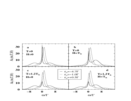
FIG. 1.: $A_{\uparrow}(\omega,T,H)$ in the Kondo ( $\varepsilon_{d}=-4.7\Gamma$), mixed valent ($\varepsilon_{d}=-\Gamma$), and empty orbital ($\varepsilon_{d}=0.5\Gamma$) regimes at $T=0$ (a-b) and at $T=1.2T_{K}$ (c-d), where $T_{K}$ is defined after Eq. (6)

For the calculations we used $U/\pi\Gamma=3$ and $\Gamma=0.01D$, with $D=1$ the half-bandwidth of the free electron reservoir, whose spectral density is taken to be independent of energy (we also set $|e|=g=\mu_{B}=k_{B}=1$ so that quantities like $H/T_{K}$, $V/\Gamma$ in the figures should be interpreted as $g\mu_{B}H/k_{B}T_{K}$ and $|e|V/\Gamma$). This choice of parameters suffices to account for all interesting effects of correlation. Depending on the dot level position, there are three regimes of interest [13]: (i) the Kondo regime, $-0.5U\leq\varepsilon_{d}\lesssim-\Gamma$, characterized by an exponentially small scale $T_{K}\sim(U\Gamma/2)^{1/2}\exp(\pi\varepsilon_{d}(\varepsilon_{d}+U)/2\Gamma U)$, (ii) the mixed valent regime $-\Gamma\lesssim\varepsilon_{d}\lesssim 0$ characterized by the charge fluctuation scale $\Gamma$ and, (iii), the empty orbital regime $\varepsilon_{d}\gtrsim 0$ characterized by a scale $\tilde{\varepsilon}_{d}\sim\varepsilon_{d}$, corresponding to the renormalized level position. The region $\varepsilon_{d}\leq-0.5U$ is related to that for $\varepsilon_{d}\geq-0.5U$ by particle-hole symmetry: ${\cal H}(\varepsilon_{d},H)\leftrightarrow{\cal H}(-(\varepsilon_{d}+U),-H)$. As a consequence we have

$$A_{\sigma}(\omega,T,H,\varepsilon_{d})=A_{-\sigma}(-\omega,T,H,-(\varepsilon_{d}+U)).$$ (6)

We use this to calculate $G,G_{\uparrow}$ and $G_{\downarrow}$ at all relevant $\varepsilon_{d}$. Throughout this paper, we define $T_{K}$ to be the HWHM of the $T=H=0$ Kondo resonance at the particle-hole symmetric point $-\varepsilon_{d}/U=0.5$ (mid-valley point in Fig. 2). It has the value $T_{K}\approx 0.001=\Gamma/10$.

FIG. 2.: Temperature and gate voltage dependence of the conductance $G(T,H)$for fields (a) $H=0$, (b) $H=0.1T_{K}$, (c) $H=T_{K}$ and $H=5T_{K}$. The symbols in (a) are the $T=0$ unitarity limit of the conductance Eq. (7). The temperatures decrease from bottom to top and correspond to $T_{N}=T_{0}\Lambda^{-N},N=0,1,2,\dots,\Lambda=1.5$ with the highest temperature being $T_{0}=1.32\Gamma$ (the dashed curves in (a-d) have $T=1.2T_{K}$). The Kondo scale, $T_{K}$, is defined after Eq. (6). The regions marked $1,2$ and $3$ in (a) and separated by vertical dashed lines correspond to the Kondo, mixed valent and empty orbital regimes respectively.

Spectral densities— Fig. 1a-d summarizes the behaviour of the spectral density $A_{\sigma}(\omega,T,H)$ in zero and finite magnetic fields which will be useful for discussing the conductance results below (for full details see [9, 10, 17]). The general trends in the Kondo regime at $H=0$ are two almost temperature independent resonances at $\omega\approx\varepsilon_{d}$ and $\omega\approx\varepsilon_{d}+U$ and a strongly temperature dependent Kondo resonance at $\omega\approx 0$ (cf. Fig. 1a,c). Fields comparable to $T_{K}$ result in a large shift of spectral weight in $A_{\uparrow}$ from the excitation at $\varepsilon_{d}$ to the one at $\varepsilon_{d}+U$ (and an opposite shift in $A_{\downarrow}$). The Kondo resonance in $A_{\uparrow}$ ($A_{\downarrow}$) shifts upwards (downwards) by an amount $\lesssim H$ and is reduced in height [10] (cf. Fig. 1a,b). In the mixed valent regime, the Kondo resonance has merged with the excitation at $\varepsilon_{d}$ to form a renormalized resonance of width $\Gamma$ lying close to but above the Fermi level at $\tilde{\varepsilon}_{d}<\Gamma/2$. The excitation at $\varepsilon_{d}+U$ has little weight. The resonance at $\tilde{\varepsilon}_{d}\approx\varepsilon_{d}$ in the empty orbital regime is almost independent of temperature and field on scales comparable to $\Gamma$ and the one at $\varepsilon_{d}+U$ is no longer discernable.

Gate voltage dependence of the conductance— The gate voltage dependence of the linear conductance is shown in Fig. 2a-d for several temperatures and magnetic field strengths. Consider first the zero field case. The charging energy, $U$, corresponds to the separation between the Coulomb blockade peaks at high temperature (these arise when $\varepsilon_{d}$ or $\varepsilon_{d}+U$ coincide with the Fermi level of the leads). On lowering the temperature these peaks move together as a result of the development of the Kondo resonance in region 1, as observed experimentally [1]. The conductance in region 1 continues to increase with decreasing temperature, eventually reaching the unitarity limit of $2e^{2}/h$, which has recently been seen in experiments [5]. As a check on our $T\rightarrow 0$ results for all $\varepsilon_{d}$ we have shown the $T=0$ unitarity curve [7, 8] (which follows from [18])

$$G(T=H=0) = \frac{2e^{2}}{h}\sin^{2}(\pi n_{d}/2),$$ (7)

with the dot level occupancy, $n_{d}$, deduced from the spectral densities. As in the experiments [1], the enhancement of the conductance with decreasing temperature in the Kondo and mixed valent regimes (regions 1 and 2 in Fig. 2) is in marked contrast to the suppression of the conductance with decreasing temperature in the empty orbital case (region 3).

FIG. 3.: Dependence of the spin-resolved conductance $G_{\uparrow}(T,H)$ on gate voltage for several magnetic fields (a-d), and for the same $T_{K}$ and temperatures as in Fig. 2. $G_{\downarrow}$ is the mirror reflection of $G_{\uparrow}$ about $\varepsilon_{d}/U=-0.5$ as described in the text.

On applying a small magnetic field we see a drastic change in the total conductance in the Kondo regime. A magnetic field suppresses the Kondo effect, tending to split the total spectral density at the Fermi level, and thereby decreases the conductance in the Kondo valley (region 1). A sizeable effect is also seen in the mixed valent regime, but very little change is observed in the empty orbital case. The effects of a magnetic field become even more apparent in spin-resolved quantities such as $G_{\uparrow}$ in Fig. 3 (from Eq. (6) $G_{\downarrow}$, as a function of $\varepsilon_{d}$, is the mirror reflection of $G_{\uparrow}$ about $\varepsilon_{d}=-0.5U$). Again, the main effect of a field is to change dramatically the conductance in the Kondo regime (region 1 of Fig. 2a) with some changes also in the mixed valent regime. The low $T$ asymmetry in the conductance $G_{\uparrow}$ about $\varepsilon_{d}=-0.5U$ at finite fields reflects the fact that the $H=0$ Kondo resonance lies just above the Fermi level for $\varepsilon_{d}>-0.5U$ but just below the Fermi level for $\varepsilon_{d}<-0.5U$. Consequently, applying a field $+H$, which moves the Kondo resonance in $A_{\uparrow}$ upwards, leads to a suppression of $G_{\uparrow}$ for the former case and an enhancement for the latter. A quantum dot in a field is seen to act as a spin-filter as discussed in [19] for dots weakly coupled to leads ($G_{\sigma}\ll e^{2}/h$). We note that the effect is largest in the mixed valent regime (see Fig. 4 below).

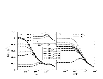
FIG. 4.: Temperature dependence of $G_{\uparrow}$ (filled symbols, solid lines) and $G_{\downarrow}$ (open symbols, dashed lines) at several values of the magnetic field for three characteristic gate voltages corresponding to (a) the Kondo regime ($\varepsilon_{d}=-4.7\Gamma$), (b), the mixed valent regime ($\varepsilon_{d}=-\Gamma$), and, (c), the empty orbital regime ($\varepsilon_{d}=+\Gamma$, symbols omitted for clarity). Dashed (solid) curves are for $G_{\downarrow}$ ($G_{\uparrow}$). The Kondo scale, $T_{K}$, is that defined in Fig. 2.

Temperature dependence of the conductance— Fig. 4 shows the temperature dependence of the spin-resolved conductance at several magnetic fields and for gate voltages corresponding to Kondo (Fig. 4a), mixed valent (Fig. 4b) and empty orbital regimes (inset to Fig. 4a). The results for the Kondo regime are similar to those calculated directly from the Kondo model [10], except that charge fluctuations, absent in the former, give rise, in the AM, to a small peak at $T\gtrsim\Gamma$ in $G_{\sigma}$. At low temperatures, $T<T_{K}$, the two spin components of the Kondo resonance move away from the Fermi level and decrease in height with increasing field [10]. This leads to the observed strong suppression of both $G_{\uparrow}(T<T_{K})$ and $G_{\downarrow}(T<T_{K})$ and to the appearance for $H\gtrsim 0.5T_{K}$ of a noticeable peak at $T\approx H$ and would be experimentally observable in transport measurements of $G(T,H)$. The behaviour in the mixed valent (Fig. 4b) and empty orbital (inset to Fig. 4a) regimes is different. $G_{\uparrow}$ is suppressed whereas $G_{\downarrow}$ is enhanced by increasing the field. This is understood by noting that for these cases, the resonance in the spectral density at $H=0$ lies above the Fermi level (see Fig. 1), and application of a field has little effect on the height of the spin components, $A_{\sigma}$, of the spectral density (in contrast to the Kondo regime). The main effect is to shift these components in opposite directions, resulting in $A_{\downarrow}(\omega=0,T=0,H)$ increasing and $A_{\uparrow}(\omega=0,T=0,H)$ decreasing with increasing field, which thereby gives rise to the opposite trends in $G_{\uparrow}$ and $G_{\downarrow}$. The main difference between the mixed valent and empty orbital cases, is the stronger field dependence of $G_{\sigma}$ for the former.

In summary we have studied magnetotransport through a strongly interacting quantum dot with one active level for transport. Quantitative agreement with the $H=0$ conductance as a function of temperature has already been demonstrated for quantum dots in heterostructures [1, 5] and more recently also for quantum dots defined in carbon nanotubes [20]. Our predictions for the conductance in a magnetic field can be directly tested with measurements on quantum dots with a field parallel to the plane of the quantum dot so that orbital effects can be neglected. Such experiments are currenlt being planned [21]. There is also much interest in realizing spin polarized currents through mesoscopic devices, such as quantum dots, so our results for spin-resolved conductances in a magnetic field could eventually be tested against experiment. Our results show that a strongly coupled quantum dot ($G_{\sigma}\sim e^{2}/h$) in a magnetic field acts as a spin-filter as found for weakly coupled ($G_{\sigma}\ll e^{2}/h$) quantum dots [19]. The largest spin-filtering effect is in the mixed valent regime.

Useful discussions with J. von Delft, S. De Franceschi, D. Goldhaber-Gordon, E. Kats, P. Krüger, D. Loss, Ph. Nozières, F. Pistolesi and E. Sukhorukov are gratefully acknowledged.

REFERENCES

- [1] D. Goldhaber–Gordon et al., Phys. Rev. Lett. 81, 5225 (1998).
- [2] S. M. Cronenwett, T. H. Oosterkamp and L. Kouwenhoven, Science 281, 540 (1998).
- [3] J. Schmid et al., Physica B 256, 182 (1998).
- [4] F. Simmel et al., Phys. Rev. Lett. 83, 804 (1999).
- [5] W. G. van der Wiel et al., Science 289, 2105 (2000).
- [6] A. C. Hewson, The Kondo Problem to Heavy Fermions (Cambridge University Press, Cambridge, England 1993)
- [7] L. I. Glazman and M. E. Raikh, Sov. Phys. JETP Lett. 47, 454 (1988).
- [8] T. K. Ng and P. A. Lee, Phys. Rev. Lett. 61, 1768 (1988).
- [9] T. A. Costi, A. C. Hewson and V. Zlatić, J. Phys. Cond. Matt. 6, 2519 (1994).
- [10] T. A. Costi, Phys. Rev. Lett. 85, 1504 (2000).
- [11] Y. Ohno et al., Nature 402, 790 (1999).
- [12] S. Hershfield, J. H. Davies and J. W. Wilkins, Phys. Rev. Lett. 67, 3720 (1991); Y. Meir, N. S. Wingreen and P. A. Lee, Phys. Rev. Lett. 70, 2601 (1993).
- [13] K. G. Wilson, Rev. Mod. Phys.47, 773 (1975); H. R. Krishna-murthy, J. W. Wilkins and K. G. Wilson, Phys. Rev. B21, 1003 (1980).
- [14] T. A. Costi, in Density Matrix Renormalization, edited by I. Peschel, X. Wang, M. Kaulke and K. Hallberg (Springer, Berlin, Germany 1999).
- [15] R. Bulla, T. A. Costi and D. Vollhardt, Phys. Rev. B 64, 045103 (2001).
- [16] R. Bulla, A. C. Hewson and Th. Pruschke, J. Phys. Cond. Matt. 10, 8365 (1998).
- [17] W. Hofstetter, Phys. Rev. Lett. 85, 1508 (2000).
- [18] D. C. Langreth, Phys. Rev. 150, 516 (1966).
- [19] P. Recher, E. V. Sukhorukov and D. Loss, Phys. Rev. Lett. 85, 1962 (2000).
- [20] J. Nygard, D. H. Cobden and P. E. Lindelof, Nature 408, 342 (2000).
- [21] D. Goldhaber-Gordon, private communication.