Bond operator mean field theory of the half filled Kondo lattice model

Abstract

We present a bond-operator mean field theory for the Kondo lattice model at half filling in two (2D) and three (3D) dimensions. A continuous quantum phase transition from an antiferromagnetic to a spin-gapped singlet ground state is found at $J/t=1.505$ ($1.833$) in $2D$ ($3D$). Additionally we evaluate the quasiparticle dispersions as well as the staggered magnetic moment and provide a comparison with complementary numerical approaches.

The Kondo Lattice Model (KLM) describes the exchange-scattering of a band of itinerant conduction-electrons at a lattice of localized magnetic moments. It serves as a basic model for heavy fermion materials in the integral-valent limit [1]. At half filling of the conduction band it is believed to give a description of Kondo insulators, which have been of considerable interest in recent years[2]. In one dimension the ground state at half filling is a spin singlet for all values of exchange-scattering and conduction-band widths[3]. In higher dimensions it has been suggested early on, that the competition between Kondo screening and the Ruderman-Kittel-Kasuya-Yoshida (RKKY) interaction leads to a quantum phase transition between a global spin-singlet and an antiferromagnetically ordered phase[4, 5]. This scenario has been corroborated in two dimensions by variational[6] calculations, series expansion[7] and mean-field[8] approaches. Numerically exact results in 2D have been obtained recently by QMC[9, 10]. In $3D$ only series expansion is available[7].

The purpose of this work is to introduce a novel mean-field theory for the KLM at half filling in two and three dimensions. In contrast to other mean-field calculations[5, 8] our approach is based on a bond-operator representation of the KLM which is suitable for strong exchange scattering and has proven to be useful in dimerized spin systems [12]. Moreover, our treatment goes beyond recent mean-field work focusing on the Kondo-necklace problem which neglects conduction-electron charge fluctuations [11]. The KLM reads

$$H=-t\sum_{\{i,j\},\sigma}c^{\dagger}_{i,\sigma}c^{\phantom{\dagger}}_{j,\sigma}+J\sum_{i}{\bf S}_{i,c}{\bf S}_{i,f}$$ (1)

with spin operators ${\bf S}_{c(f)}=\frac{1}{2}\sum_{\sigma,\sigma^{\prime}}c(f)^{\dagger}_{\sigma}\tau_{\sigma,\sigma^{\prime}}c(f)^{\phantom{\dagger}}_{\sigma^{\prime}}$ and destruction(creation) operators $c^{(\dagger)}_{i,\sigma}$ and $f^{(\dagger)}_{i,\sigma}$ for itinerant $c$ and localized $f$ electrons of spin $\sigma$ at sites $i$. An f-occupation of exactly one per lattice site is implied.

The local Hilbert space consists of one $f$ electron with spin up or down and additionally up to two itinerant electrons. The resulting eight possible states can be created by applying the following operators onto the vacuum $|0\rangle$ of an empty site

$$s^{\dagger}|0\rangle = \frac{1}{\sqrt{2}}(c^{\dagger}_{\uparrow}f^{\dagger}_{\downarrow}+f^{\dagger}_{\uparrow}c^{\dagger}_{\downarrow})|0\rangle$$ (2)

$$t^{\dagger}_{x}|0\rangle = \frac{-1}{\sqrt{2}}(c^{\dagger}_{\uparrow}f^{\dagger}_{\uparrow}-c^{\dagger}_{\downarrow}f^{\dagger}_{\downarrow})|0\rangle$$ (3)

$$t^{\dagger}_{y}|0\rangle = \frac{i}{\sqrt{2}}(c^{\dagger}_{\uparrow}f^{\dagger}_{\uparrow}+c^{\dagger}_{\downarrow}f^{\dagger}_{\downarrow})|0\rangle$$ (4)

$$t^{\dagger}_{z}|0\rangle = \frac{1}{\sqrt{2}}(c^{\dagger}_{\uparrow}f^{\dagger}_{\downarrow}+c^{\dagger}_{\downarrow}f^{\dagger}_{\uparrow})|0\rangle$$ (5)

$$a^{\dagger}_{\sigma}|0\rangle = f^{\dagger}_{\sigma}|0\rangle$$ (6)

$$b^{\dagger}_{\sigma}|0\rangle = c^{\dagger}_{\uparrow}c^{\dagger}_{\downarrow}f^{\dagger}_{\sigma}|0\rangle.$$ (7)

where the operators $s$ and $t$ are equivalent to the so-called bond operators of[12] and are assumed to obey bosonic commutation relations. The fermionic operators $a$ and $b$ have been introduced first in[13] and label states with one or three electrons per site. In order to suppress unphysical states a constraint of no double occupancy

$$s^{\dagger}_{j}s^{\phantom{\dagger}}_{j}+\sum_{\alpha}t^{\dagger}_{\alpha,j}t^{\phantom{\dagger}}_{\alpha,j}+\sum_{\sigma}a^{\dagger}_{\sigma,j}a^{\phantom{\dagger}}_{\sigma,j}+\sum_{\sigma}b^{\dagger}_{\sigma,j}b^{\phantom{\dagger}}_{\sigma,j}=1$$ (8)

has to be fulfilled. The original fermion and spin operators are represented by

$$c^{\dagger}_{j,\sigma}=p_{\sigma}\frac{1}{\sqrt{2}}[(s^{\dagger}_{j}+p_{\sigma}t^{\dagger}_{z,j})a^{\phantom{\dagger}}_{-\sigma,j}-(t^{\dagger}_{x,j}+p_{\sigma}it^{\dagger}_{y,j})a_{\sigma,j}]$$ (9)

$$-\frac{1}{\sqrt{2}}[b^{\dagger}_{\sigma,j}(s^{\phantom{\dagger}}_{j}-p_{\sigma}t^{\phantom{\dagger}}_{z,j})-b^{\dagger}_{-\sigma,j}(t_{x,j}^{\phantom{\dagger}}+p_{\sigma}it_{y,j}^{\phantom{\dagger}})]$$ (10)

$$S^{c}_{\alpha,j} = \frac{1}{2}(-t^{\dagger}_{\alpha,j}s^{\phantom{\dagger}}_{j}-s^{\dagger}_{j}t^{\phantom{\dagger}}_{\alpha,j}-i\sum_{\beta,\gamma}\epsilon_{\alpha\beta\gamma}t^{\dagger}_{\beta,j}t^{\phantom{\dagger}}_{\alpha,j})$$ (11)

$$S^{f}_{\alpha,j} = \frac{1}{2}(t^{\dagger}_{\alpha,j}s^{\phantom{\dagger}}_{j}+s^{\dagger}_{j}t^{\phantom{\dagger}}_{j}-i\sum_{\beta,\gamma}\epsilon_{\alpha\beta\gamma}t^{\dagger}_{\beta,j}t^{\phantom{\dagger}}_{\alpha,j})$$ (12)

$$+ S^{a}_{\alpha,j}+S^{b}_{\alpha,j}$$ (13)

with ${\bf S}_{a(b),j}=\frac{1}{2}\sum_{\sigma,\sigma^{\prime}}a(b)^{\dagger}_{\sigma,j}\tau_{\sigma,\sigma^{\prime}}a(b)^{\phantom{\dagger}}_{\sigma^{\prime},j}$ and $p_{\uparrow}=1$, $p_{\downarrow}=-1$. This mapping is exact and preserves the proper commutation relations provided that $s$ and $t$ are bosons, $a$ and $b$ are fermions, and (8) is satisfied.

Rewriting the KLM in terms of (8,10-13) leads to a strongly correlated boson-fermion model which cannot be solved exactly, but approximations have to be made. Analogous models in the context of quantum-disordered ground states in dimerized spin systems have recently been treated by various schemes of approximation [14, 15, 16, 17]. Here we are interested in a mean-field description of the transition from an antiferromagnetic state to a spin-singlet regime. The latter can be described by allowing for a condensate of singlets[12]

$$\langle s^{\phantom{\dagger}}_{j}\rangle=\langle s^{\dagger}_{j}\rangle=s$$ (14)

while the antiferromagnetically ordered phase requires an additional condensation of one of the triplets [18]

$$\langle t^{\phantom{\dagger}}_{z,j}\rangle=\langle t^{\dagger}_{z,j}\rangle=m_{j}=(-1)^{j}m$$ (15)

For the remainder of this work we assume a bipartite lattice structure with the factor of $(-1)^{j}$ being a shorthand for ’$+1(-1)$’ on the A(B) sublattice.

Inserting (14,15) into (10-13) and (1) we drop all longitudinal and transverse spin-fluctuations, i.e., we only keep the mean-field values of $s$ and $t$ in addition to the fermions $a$ and $b$. We obtain

$$H = -\frac{t}{2}\sum_{\{i,j\},\sigma}(-sp_{\sigma}+m_{i})(-sp_{\sigma}+m_{j})\times$$ (22)

$$\qquad\times(a^{\phantom{\dagger}}_{\sigma,i}a^{\dagger}_{\sigma,j}+b^{\dagger}_{\sigma,i}b^{\phantom{\dagger}}_{\sigma,j})+h.c.$$

$$-\frac{t}{2}\sum_{\{i,j\},\sigma}(-sp_{\sigma}+m_{i})(sp_{\sigma}+m_{j})\times$$

$$\qquad\times(-p_{\sigma}a^{\phantom{\dagger}}_{\sigma,i}b^{\phantom{\dagger}}_{-\sigma,j}+p_{\sigma}b^{\dagger}_{\sigma,i}a^{\dagger}_{-\sigma,j})+h.c.$$

$$-\frac{3}{4}JNs^{2}+\frac{1}{4}JNm_{i}^{2}$$

$$+\sum_{i,\sigma}\mu_{i}(s^{2}+m_{i}^{2}+a^{\dagger}_{\sigma,i}a^{\phantom{\dagger}}_{i,\sigma}+b^{\dagger}_{\sigma,i}b^{\phantom{\dagger}}_{\sigma,i}-1)$$

$$+\lambda\sum_{i,\sigma}(b^{\dagger}_{\sigma,i}b^{\phantom{\dagger}}_{\sigma,i}-a^{\dagger}_{\sigma,i}a^{\phantom{\dagger}}_{\sigma,i})$$

The first sum $\propto t$ describes hopping of particle- or hole-like fluctuations with a dispersion renormalized by a factor of $(s^{2}-m^{2})$, taking into account the alternation of the sign of $m_{i}$. This prefactor leads to a reduction of the fermionic kinetic energy in the antiferromagnetic phase. The second sum $\propto t$ generates the mean-field analog of the intermediate state of the RKKY process and its hermitian conjugate, i.e., the destruction(creation) of two adjacent two-particle states accompanied by the creation(destruction) of a pair of two adjacent three- and one-electron states. Second order processes from this term drive the transition into the magnetic state. Thus we believe that this mean-field Hamiltonian incorporates the basic ingredients to induce the quantum-phase transition of the KLM. Furthermore in (22) we have introduced the usual chemical potential $\lambda$ to set the global particle density and a local Lagrange multiplier $\mu_{i}$ in order to to enforce the constraint (8).

To diagonalize the Hamiltonian we first replace the local Lagrange multiplier by a global one $\mu_{i}\rightarrow\mu$. Second we switch to an antiferromagnetic unit cell and finally perform a generalized Bogoliubov transformation to eliminate particle-number non-conserving term of type $ab(a^{\dagger}b^{\dagger})$. This leads to $4$ bands $\omega_{1,2}({\bf k})=\lambda\pm E_{1}({\bf k})$ and $\omega_{3,4}({\bf k})=\lambda\pm E_{2}({\bf k})$ which are twofold degenerate by spin-z quantum number

$$E_{1,{\bf k}} = \sqrt{\mu^{2}+\frac{1}{2}\epsilon_{\bf k}^{2}(m^{2}+s^{2})^{2}-2W_{\bf k}}$$ (23)

$$E_{2,{\bf k}} = \sqrt{\mu^{2}+\frac{1}{2}\epsilon_{\bf k}^{2}(m^{2}+s^{2})^{2}+2W_{\bf k}}$$ (24)

$$W_{\bf k} = \sqrt{\frac{1}{4}\mu^{2}(m^{2}-s^{2})^{2}\epsilon_{\bf k}^{2}+\frac{1}{16}\epsilon_{\bf k}^{4}(m^{2}+s^{2})^{4}}$$ (25)

Here $\epsilon_{\bf k}=-2t\sum_{d=1}^{D}\cos k_{d}$. At half filling the lower two bands, i.e. $\omega_{2,4}$, are completely filled while the upper two bands , i.e. $\omega_{1,3}$, are empty. This leads to a ground state energy of

$$\frac{E}{N} = -\frac{3}{4}Js^{2}+\frac{1}{4}Jm^{2}+\mu(s^{2}+m^{2}+1)$$ (27)

$$-\frac{1}{2N}\sum_{\bf k}2E_{1,{\bf k}}-\frac{1}{2N}\sum_{\bf k}2E_{2,{\bf k}}$$

which is independent of $\lambda$.

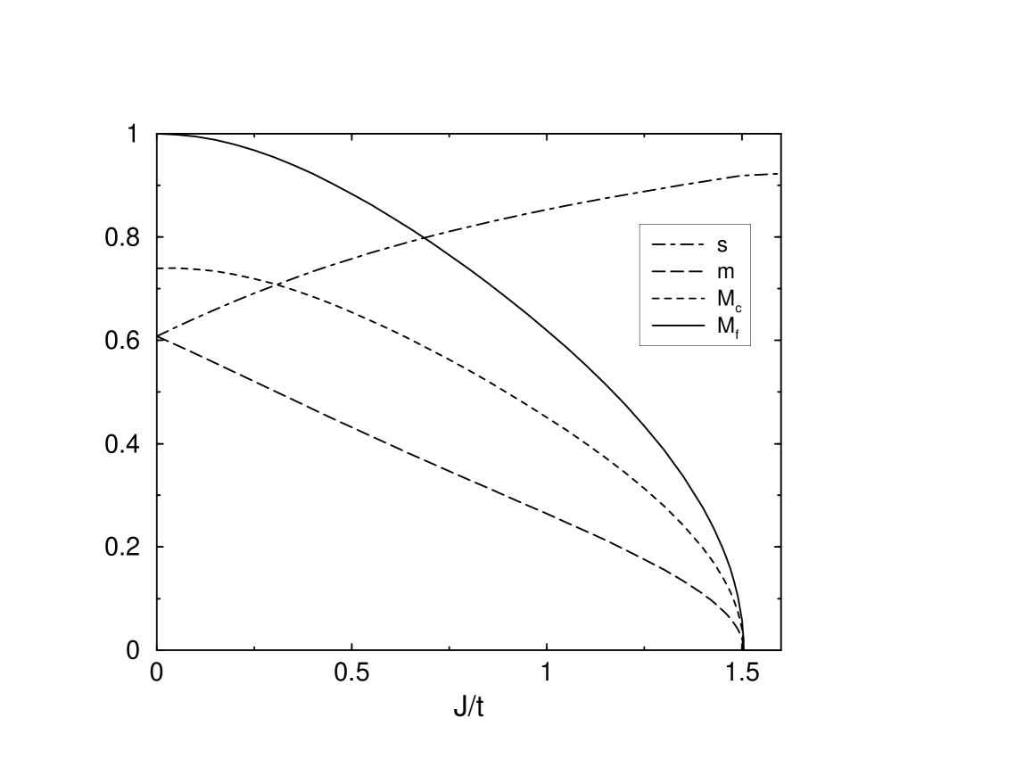
FIG. 1.: Mean-field order parameter $s$, $m$ and the staggered moments $M_{c}$ and $M_{f}$ as function of $J/t$ for the $2D$ KLM.

The staggered magnetization $M_{c(f)}$ of the $c(f)$ electrons is obtained from a direct evaluation of the corresponding matrix elements in the mean-field ground state

$$M_{c} = \frac{2}{N}\sum_{n}(-1)^{n}\langle S^{c}_{z,n}\rangle=2ms$$ (28)

$$M_{f} = \frac{2}{N}\sum_{n}(-1)^{n}\langle S^{f}_{z,n}\rangle=$$ (29)

$$= 2ms+\frac{1}{N}\sum_{\bf k}\frac{2\epsilon_{\bf k}^{2}\mu ms(s^{2}+m^{2})}{E_{1,{\bf k}}E_{2,{\bf k}}(E_{1,{\bf k}}+E_{2,{\bf k}})}.$$ (30)

The second term in $M_{f}$ is due to a staggering of the spin density of the $a$ and $b$ fermions which develops at non-zero values of $m$ due to the the second sum $\propto t$ in (22). This terms induces a spin-dependent non-diagonal momentum-space component in the $a$ and $b$ Greens functions at the antiferromagnetic nesting wave-vector.

The mean-field equations

$$\frac{\partial E}{\partial s}=0\qquad\frac{\partial E}{\partial m}=0\qquad\frac{\partial E}{\partial\mu}=0$$ (31)

have to be solved self-consistently for the order parameters $s$, $m$ and $\mu$. In the magnetic phase ($m\neq 0$) the system of equations (31) can be written as

$$0 = 2J+\frac{1}{2N}\sum_{\bf k}\frac{\epsilon_{\bf k}^{2}\mu^{2}(s^{2}-m^{2})}{W_{\bf k}}\left(\frac{2}{E_{2,{\bf k}}}-\frac{2}{E_{1,{\bf k}}}\right)$$ (32)

$$0 = -J+4\mu-\frac{1}{2N}\sum_{\bf k}2\epsilon_{\bf k}^{2}(m^{2}+s^{2})\left(\frac{2}{E_{2,{\bf k}}}+\frac{2}{E_{1,{\bf k}}}\right)$$ (34)

$$-\frac{1}{2N}\sum_{\bf k}\frac{\epsilon_{\bf k}^{4}(m^{2}+s^{2})^{3}}{2W_{\bf k}}\left(\frac{2}{E_{2,{\bf k}}}-\frac{2}{E_{1,{\bf k}}}\right)$$

$$0 = s^{2}+m^{2}+1-\frac{1}{2N}\sum_{\bf k}\mu\left(\frac{2}{E_{2,{\bf k}}}+\frac{2}{E_{1,{\bf k}}}\right)$$ (36)

$$-\frac{1}{2N}\sum_{\bf k}\frac{\epsilon_{\bf k}^{2}\mu(s^{2}-m^{2})^{2}}{4W_{\bf k}}\left(\frac{2}{E_{2,{\bf k}}}-\frac{2}{E_{1,{\bf k}}}\right)\;\;,$$

while for the disordered one ($m=0$) it simplifies considerably

$$0 = -\frac{3}{2}J+2\mu-\frac{1}{N}\sum_{\bf k}\frac{2\epsilon_{\bf k}^{2}s^{2}}{\sqrt{4\mu^{2}+\epsilon_{k}^{2}s^{4}}}$$ (37)

$$0 = s^{2}+1-\frac{1}{N}\sum_{\bf k}\frac{4\mu}{\sqrt{4\mu^{2}+\epsilon_{\bf k}^{2}s^{4}}}.$$ (38)

For $\epsilon_{\bf k}=0$, i.e. $t=0$, only (38) has a solution. This solution also provides for the correct quasiparticle gap, i.e. $\mu=\frac{3}{4}J$. Upon increasing $t$ charge fluctuations, i.e. creation of $a$- and $b$-excitations contribute to the ground state reducing the stability of the singlet state. At $J/t\rightarrow 0$ the ground state stems from the solution of (36) with $s=m$. This state displays a complete polarization of the $f$ spins, while the $c$ spin density is polarized only partially. The latter is consistent with the itinerant character of the $c$ fermions, implying a finite density of empty and doubly occupied sites, i.e. a finite density of $a$ and $b$ fermions. Since $s=m$ at $J/t=0$ the diagonal part of the kinetic energy of the $a$ and $b$ particles vanishes at this point.

At intermediate $J/t$ we determine the ground state by solving (36,38) numerically. Fig. 1 shows the singlet and triplet order parameters as well as the staggered magnetizations for the $2D$ KLM. We observe a continuous quantum phase transition from the singlet to the magnetic phase at $(J/t)_{c}=1.505$. This is in good agreement with the data of a recent QMC study[9] which has determined the phase transition to occur at $(J/t)_{c}=1.45\pm 0.05$. Similar values of $(J/t)_{c}$ have also been reported from variational Monte-Carlo simulations[6] ($(J/t)_{c}=1.4\pm 0.1$) and series expansion[7]($(J/t)_{c}=1.43\pm 0.2)$. From Fig. 1 it can be seen that the maximum magnetization, i.e. $s=m$, prevails only at $J=0$ with a continuous increase of $s$ vs. $m$, i.e. screening of the local moment, to occur as $J$ approaches $J_{c}$. Such coexistence of Kondo screening and antiferromagnetic order has also been reported recently from QMC calculations[10] for all $J<J_{c}$ and within a small window of values of $J$ from a mean-field study[8].

FIG. 2.: Quasiparticle dispersions for (a) J/t=1.2 and (b) J/t=2.

Fig. 2 shows the quasiparticle dispersion of the occupied bands for two values of $J/t$ which are in the singlet and the magnetic phase, i.e. (a) $J/t=2$ and (b) $J/t=1.2$ respectively. These bands are split by a gap from the unoccupied bands which are located symmetrically reflected along the line $E/t=0$ at positive energies. For $J>J_{c}$ the four bands $\omega_{1...4}({\bf k})$ collapse onto only two bands by a mere backfolding which has been carried out in fig. 2(a) leaving a single occupied band to be displayed. For $J<J_{c}$ two distinct bands are present throughout the entire magnetic Brillouin zone. Since the Hamiltonian (22) incorporates scattering with a magnetic wave-vector ${\bf k}=(\pi,\pi)$ in the off-diagonal terms only, no additional gap opens along the line ${\bf k}_{N}$ with $k_{N,x}+k_{N,y}=\pi$, i.e. $W_{{\bf k}_{N}}=0$ in (25). In this context we note, that the interpretation of the band-gap in this mean-field theory changes quasi-continuously from a gap induced by singlet formation at $J>J_{c}$ to a magnetic gap as $J\rightarrow 0$.

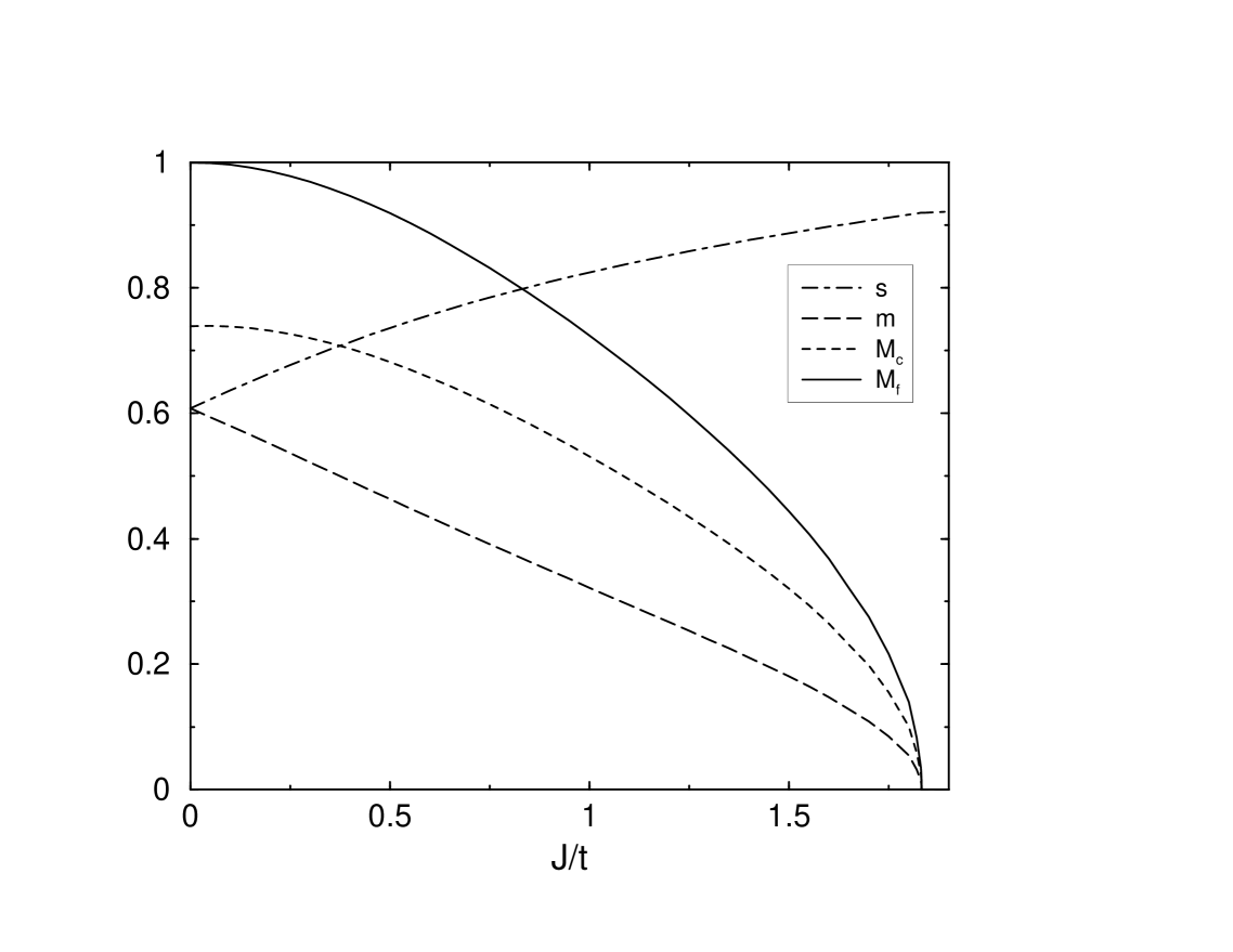
FIG. 3.: Mean-field order parameter $s$, $m$ and the staggered moments $M_{c}$ and $M_{f}$ as function of $J/t$ for the $3D$ KLM.

In fig. 3 we display a set of results identical to that of fig. 1 however for the 3D case. Here the phase transition occurs at a slightly larger value of $(J/t)_{c}=1.833$, which is in reasonable agreement with an estimate of $(J/t)_{c}=2.04\pm 0.16$ reported from series expansion[7]. Again, the $f$ spins are fully polarized as $J\rightarrow 0$, while the maximum value of $M_{c}$ is nearly identical to that of the $2D$ case.

To conclude several comments are in order. First, and very much in contrast to usual approaches to the KLM [5, 1] our method is best suited for the limit of strong and quasi local Kondo screening at large $J/t$. In that limit the Kondo effect can be viewed as a molecular singlet formation within each unit cell resulting in an algebraic energy scale of order $J$, rather than the usual Kondo energy-scale $T_{K}\sim t\exp(-t/J)$. While the large-$J$ limit may obliterate some of the subtleties genuine to the Kondo effect at $J\ll t$, we believe that it is a superior starting point for analytic studies of the quantum phase transition in the 2D and 3D KLM since this transition occurs at $J/t>1$. Second, we note that while we have neglected quantum fluctuations of the triplet order parameter, it would be interesting to incorporate them into future studies. In particular, it is conceivable that transverse fluctuations due to the $t_{x,y}$-operators will reduce the staggered magnetization in the ordered phase. This seems consistent with QMC finding a smaller magnetization[9] than we observe within the mean-field approach. Finally an extension of the scheme presented here to incorporate Coulomb correlations or finite doping, off half filling, into the conduction band are open issues.

In summary we have studied the KLM using a novel bond-operator mean-field theory. In good agreement with complementary approaches we find a quantum phase transition at $(J/t)_{c}=1.505(1.833)$ in 2(3) dimensions. In addition we have evaluated the magnetization in the ordered phase and the quasiparticle dispersions.

This research was supported in part by the Deutsche Forschungsgemeinschaft under Grant No. BR 1084/1-1 and BR 1084/1-2.

REFERENCES

[1]
P. Fulde, J. Keller, G. Zwicknagl, Solid State Phys. 41,1 (1988).
[2]
G. Aeppli, Z. Fisk, Comments Condens. Matter Phys. 16, 155.
[3]
H. Tsunetsugu, M. Sigrist, K. Ueda, Rev. Mod. Phys. 69,809 (1997).
[4]
S. Doniach, Physica B 91, 231 (1977).
[5]
C. Lacroix, M. Cyrot Phys. Rev. B 20, 1969 (1979).
[6]
Z. Wang, X. Li, D.-H. Lee, Physica B 199-200, 463 (1994).
[7]
Z.-P. Shi, R. R. P. Singh, M. P. Gelfand, Z. Wang,
Phys. Rev. B 51, 15630 (1995).
[8]
G.-M. Zhang, L. Yu, Phys. Rev. B 62, 76 (2000).
[9]
F. F. Assaad, Phys. Rev. Lett. 83, 796 (1999).
[10]
S. Capponi and F. F. Assaad, cond-mat/0010393
[11]
G.-M. Zhang, Q. Gu and L. Yu, Phys. Rev. B62, 69 (2000).
[12]
S. Sachdev and R. N. Bhatt, Phys. Rev. B 41, 9323 (1990).
[13]
R. Eder, O. Stoica, and G. A. Sawatzky, Phys. Rev. B 55, 6109 (1997).
R. Eder, O. Rogojanu, and G. A. Sawatzky, Phys. Rev. B 58, 7599 (1998).
[14]
S. Gopalan, T. M. Rice, M. Sigrist, Phys. Rev. B 49, 8901
(1994).
[15]
C. Jurecka and W. Brenig, Phys. Rev. B 63, 094409 (2001).
[16]
R. Eder, Phys. Rev. B 57, 12832 (1998).
[17]
V. N. Kotov, O.P. Sushkov, Z. Weihong, and J. Oitmaa,
Phys. Rev. Lett. 80, 5790 (1998).
[18]
B. Normand and T. M. Rice, Phys. Rev. B 56, 8760 (1997).
[19]
T. Barnes, E. Dagotto, J. Riera, E. S. Swanson,
Phys. Rev. B47,3196 (1993).
[20]
M. Reigrotzki, H. Tsunetsugu and T. M. Rice,
J. Phys.: Condens. Matter 6,9235 (1994).