Constraints, Histones, and the 30 Nanometer Spiral

Abstract

We investigate the mechanical stability of a segment of DNA wrapped around a histone in the nucleosome configuration. The assumption underlying this investigation is that the proper model for this packaging arrangement is that of an elastic rod that is free to twist and that writhes subject to mechanical constraints. We find that the number of constraints required to stabilize the nuclesome configuration is determined by the length of the segment, the number of times the DNA wraps around the histone spool, and the specific constraints utilized. While it can be shown that four constraints suffice, in principle, to insure stability of the nucleosome, a proper choice must be made to guarantee the effectiveness of this minimal number. The optimal choice of constraints appears to bear a relation to the existence of a spiral ridge on the surface of the histone octamer. The particular configuration that we investigate is related to the 30 nanometer spiral, a higher-order organization of DNA in chromatin.

I Introduction

The issue of DNA packaging has been the subject of intense research for the past forty years. The remarkable fact that a meter of DNA (the total length of the human genome) fits into a cell nucleus having a typical radius of a few microns, and that, thus packed, still manages to perform all its biological functions, has captured the attention and continues to challenge the ingenuity of researchers. The fundamental unit of DNA packing in eukaryotes is the nucleosome [1, 2]. In the nucleosome configuration, a portion of the DNA strand wraps approximately one and three quarter times around a protein spool, known as a histone [3, 4, 5]. A string of nucleosomes is believed to participate in the next higher order of DNA packing by folding to form the so-called 30-nm fiber [6]. Even higher orders of organization have been conjectured, but as yet there is nothing approaching a complete understanding of the physical structure, at all orders, of the DNA in the cell nucleus. Indeed, the detailed oragnization of DNA and proteins in the 30 nm fiber is not entirely settled [7, 8, 9, 10].

In this paper, our ultimate focus will be on a single nucleosome. We will present a model for the action of histones in nucleosomes. We treat the segment of DNA in a nucleosome as an elastic rod and apply an approach first developed by Kirchhoff [11] to obtain the equilibrium configurations of DNA in the absence of histones. We assess the stability of the elastic rod with respect to small deviations from the equilibrium configurations, and we find that all configurations that are not equivalent to a straight rod are unstable to fluctuations. More specifically, all non-trivial equilibrium configurations represent saddle-points in energy space. Then we prove that the presence of histones provides a physical mechanism by which more compact configurations of DNA are rendered stable against purely mechanical fluctuations. The specific mechanism is a set of constraints on the fluctuations about mechanical equilibrium, which can be simply modeled mathematically. The stability of the equilibrium configuration is then framed in terms of the determinant of an $n$-by-$n$ matrix, where $n$ is the number of constraints. Of special interest to us is the question of the most economical combination of constraints that serves to stabilize a given configuration. “Economy” in this case refers to the number of constraints required to accomplish stabilization. We are able to establish in the case of particular interest to us that a nucleosome-like configuration of DNA is rendered stable by four constraints, and that no fewer constraints will accomplish this.

The conjecture that underlies the work reported here is that the portion of DNA that is wrapped around a histone is in a state of unstable mechanical equilibrium that is rendered mechanically stable by the constraints associated with the histone spool. There are reasons to believe that such a state is desirable. Imagine a pencil standing vertically on its point. While this state will not persist in the absence of outside influences, it can be sustained without application of substantial external forces. In fact, no force at all is required to guarantee the persistence of this state if the pencil is exactly vertical. By the same token, the removal of the constraint that keeps the vertically balanced pencil from toppling is accomplished at no energetic cost. Viewed in this way, the nucleosome configuration represents a highly efficient stratagem for the local packing of DNA, in that the histone spool is introduced and removed with minimal expenditure of resources.

Of course, because DNA is, in its “naked” state, highly charged, electrostatic interactions play an important role in the behavior of this molecule, both in vitro and in vivo. These interactions are, apparently, key to the condensation of DNA in prokaryotes [12]. Furthermore, electrostatic interactions, highly screened though they may be, could be important contributors to the energetics of the DNA-histone interactions. They are ignored in this work. Nevertheless, the elucidation of the stabilization of configurations within the context of the purely elastic model of DNA ought to aid in the investigation of similar questions for DNA subject to the influence of additional interactions and degrees of freedom.

An outline of the paper is as follows. In Section II the Hamiltonian governing configurations of DNA, modeled as a bent and twisted rod, is presented, along with the quadrature solutions to the extremum equation for that Hamiltonian. Section III reviews the formulation of linear stability analysis in this case. A key result of the considerations outlined in this section is that any non-trivial extremal configuration of bent and twisted DNA will be mechanically unstable if the strand is long enough, and if there are no constraints on fluctuations. This means that all extremum solutions for an infinite strand of bent and twisted DNA represent saddle points of the energy. Section IV introduces the notion of mechanical constraints, particularly those constraints associated with the requirement that the straight-line distance between two points on the DNA does not change as the segment fluctuates. The way in which this and other constraints are mathematically implemented is discussed in this section, and in Appendix A. In section V we address the issue of the number of constraints required to stabilize a section of bent and twisted rod against fluctuations about an extremum solution. We find that the minimum number of constraints needed to do this is equal to the number of unstable eigenmodes of a fluctuation operator introduced in Section III. Section VI contains a discussion of the effects of a periodic array of constraints on the stability of an infinitely long section of bent and twisted rod. This discussion provides a lead-in to our investigation into the influences required to stabilize the nucleosomal configuration of DNA. It is also relevant to the stabilizing action of a protein armature on DNA in chromatin. Sections VII and VIII directly address the issue of the stabilization of DNA in the nucleosomal configuration. There are four unstable modes in the case that we investigate. We find that four constraints suffice to counteract them. However, we also find that those constraints must be chosen with care. The effective set reflects the known structure of histone, in particular a spiral groove that has been identified. In our model, this groove acts to limit the ability of the DNA wrapped around it to slide parallel to the spool’s axis.

II Hamiltonian and extremum solutions

The configuration of the twisted, writhing rod is characterized in terms of the Euler angles, depicted in Figure 1. We assume an isotropic rod, characterized by a bending modulus $A$ and a torsional modulus $C$. The elastic energy of the rod, in terms of the Euler angles $\theta(s)$, $\phi(s)$ and $\psi(s)$, is given by

$$E_{\rm elastic}=\int\left\{\frac{A}{2}\left[\left(\frac{d\theta(s)}{ds}\right)^{2}+\sin^{2}\theta(s)\left(\frac{d\phi(s)}{ds}\right)^{2}\right]+\frac{C}{2}\left[\frac{d\psi(s)}{ds}+\cos\theta(s)\frac{d\phi(s)}{ds}\right]^{2}\right\}ds$$ (1)

Here, $s$ is the arclength along the rod. A way to determine the equilibrium configurations of the rod is to supplement $E_{\rm elastic}$ with the term

$$E_{c}=-F\int\cos\theta(s)ds$$ (2)

This contribution can either be seen as a Lagrange multiplier that enforces a given end-to-end distance, or as representing the effect of tension on the rod.

Finally, in certain cases an additional constraint guarantees constancy of the end-to-end linking number. In the case of a rod with clamped ends, this quantity is given by

$$Lk=-\frac{1}{2\pi}\int\left(\frac{d\phi(s)}{ds}+\frac{d\psi(s)}{ds}\right)ds$$ (3)

Note that (3) is an integral over a perfect differential. This reflects the topological character of the linking number. A fixed linking number is enforced with the use of a Lagrange multiplier. The quantity to be minimized is, then, the combination

$$E_{\rm elastic}+E_{c}-\lambda Lk$$ (4)

As the linking number is not a quantity of interest here, we ignore the final term in (4).

The extremum equations have been extensively investigated [13]. They are identical to the equations for the behavior of the heavy symmetric top. The connection between top motion and the deformations of a thin rod was first noted by Kirchhoff, in 1859 [11], and is known as the “kinetic analogue” [14]. Those equations reduce to the following set of three:

$$\frac{d\phi}{ds} = \frac{J_{\phi}-J_{\psi}\cos\theta}{A\sin^{2}\theta}$$ (5)

$$\frac{d\psi}{ds} = \frac{J_{\psi}}{C}-\frac{d\phi}{ds}\cos\theta$$ (6)

$$\sqrt{\frac{A}{2}}\frac{d\theta}{ds} = \sqrt{-\frac{\left(J_{\phi}-J_{\psi}\cos\theta\right)^{2}}{2A\sin^{2}\theta}+E_{0}-F\cos\theta}$$ (7)

The quantities $J_{\phi}$, $J_{\psi}$ and $E_{0}$ in the above equations are integration constants. The quadrature result for the angle $\theta$ is the result of integration of $\delta E_{tot}/\delta\theta$. Defining $u\equiv\cos\theta$, the behavior of solutions can be extracted from the equation for $\theta$:

$$ds=\frac{du}{\sqrt{\frac{2\left(1-u^{2}\right)}{A}\left(E_{0}-Fu\right)-\frac{1}{A^{2}}\left(J_{\phi}^{2}+J_{\psi}^{2}-2J_{\phi}J_{\psi}u\right)}}\\ \equiv\frac{du}{\sqrt{\frac{2F}{A}(u-a)(u-b)(u-c)}}\\$$ (8)

where $c<u<b<a$. The characteristics of the solutions depend on quantities $a,b$ and $c$. The property of solutions have been completely investigated [15] for different values of $a,b$ and $c$. We focus our attention on those configurations which have the same configurational form as a segment of DNA in a nucleosome. For specific value of $a,b$ and $c$ we have obtained a solution which is depicted in Figure 2. The reason that we have made the choice of parameters above has to do with the close visual relationship between the conformation of the bend and twisted rod as displayed in Fig. 2 and the DNA in a commonly conjectured form of the 30-nm spiral [6]. We operate here under the assumption that this configuration is a reasonable representation of the organization of DNA in this component of chromatin.

III Stability determination

The stability of an extremum configuration is determined by altering the configuration and calculating the change in the quantity that is extremized. In this case, the quantity of interest is the elastic energy. A stable solution is one that minimizes the energy. If the quadratic effect of any small deviation from this solution is to lower the energy, then the solution cannot represent stable equilibrium. Instead, the configuration is unstable; it is either a maximum energy configuration, or a configuration at a saddle point of the energy. In the case of the equations for the elastic energy of a twisted and bent rod, the second order effect of second order fluctuations is obtained by taking second functional derivatives of the expression in Eq. (1) with respect to the Euler angles $\theta$, $\phi$ and $\psi$, and then by setting those Euler angles equal to their classical values. After a bit of reduction, we find that the question of the stability of a classical configuration can be framed in terms of the spectrum of the following operator [16]

$$-\frac{d^{2}}{ds^{2}}+V(s)$$ (9)

where

$$V(s)=-\frac{1}{4}\frac{x(s)}{\left(1-u(s)^{2}\right)^{2}}+\frac{1}{2}u(s)$$ (10)

and

$$x(s) = \left(2-u(s)\right)\left(1-u(s)\right)^{2}(a+1)(b+1)(c+1)$$ (12)

$$+\left(2+u(s)\right)\left(1+u(s)\right)^{2}(a-1)(1-b)(1-c)$$

Here, $u(s)$ is the solution for $\cos\theta(s)$ displayed implicitly in Eq. (8). If all eigenvalues of the operator (9) are positive, then the solution to the classical equation is stable. If any is negative, then there are fluctuations that decrease the energy to a value below its classical value. Note that the operator in question resembles the Hamiltonian for a one-dimensional particle in the potential $V(s)$. In figure 3, we display this potential for the choice of parameters $a$, $b$ and $c$ utilized in this investigation. The potential, which has been displayed for an extended range of the arclength, $s$, has the form of the sort of periodic potential encountered in discussions of electrons in metals and semiconductors. As in this case, the eigenvalue spectrum consists of bands of “allowed” states, separated by “forbidden regions.” The question is whether all or part of any of the bands lie below zero. As it turns out, this is, indeed, the case.

The reason for this is that one can identify a mode having an eigenvalue that is strictly equal to zero—the translational mode, equal to the derivative with respect to $s$ of the classical solution, $\theta_{\rm cl}(s)$. The existence of this mode follows from the translational invariance of the extremum equations, and it is known to play a key role in, for instance, the question of tunneling between the false and the true vacuum in quantum field theories [17]. The translational mode in this case is displayed in Figure 4. Note that this mode is not spatially uniform, and, in particular, that it possesses nodes. On the basis of elementary considerations, one knows that there are, as a result, solutions to the effective Schrödinger’s equation associated with lower—hence negative—eigenvalues. Figure 5 displays the band structure associated with the potential in Figure 3. In an infinitely long section of twisted and bent rod that has taken the configuration pictured in Figure 2, there is an infinitely large set of distortions that will lead to a lowering of the rod’s total elastic energy. In fact, the reasonable expectation is that these distortions are a route to interwinding.

IV The sources and mathematical implementation of physical constraints

Stabilization of the classical, or extremum, configuration can be achieved by the introduction of mechanical constraints. These constraints are expressed mathematically as the requirement that a property of the DNA’s configuration does not change under distortions about the extremum solution. The physical constraint that a certain quantity be kept constant translates fairly straightforwardly into a set of mathematical conditions on the fluctuation spectrum. In turn, these mathematical restrictions lead to a reformulation of the method by which the fluctuation spectrum is determined. The reasoning leading from physical constraints to a new approach to the determination of effective eigenvalues of the linear fluctuation energy operator is presented in Appendix A.

Briefly, a constraint on the conformation of a bent and twisted rod is expressed mathematically in terms of a condition of the form

$$\int{\cal F}\left(\theta(s),\phi(s),\psi(s)\right)ds={\rm a\ constant}$$ (13)

Under the assumption that Eq. (13) is satisfied for the extremal configuration, one then expands to the first order in deviations from the extremal forms of $\theta(s)$, $\phi(s)$ and $\psi(s)$. As it turns out, the first order corrections to $\phi(s)$ and $\psi(s)$ are readily expressed in terms of the correction to $\theta(s)$. This is because of the simple way in which these two angles enter into the expression for the total energy in Eq. (1). If we denote by $\gamma(s)$ the displacement of $\theta(s)$ from its “classical” form, the general constraint equation, (13) becomes

$$\int f(\theta_{\rm cl}(s),\phi_{\rm cl}(s),\psi_{\rm cl}(s))\gamma(s)ds=0$$ (14)

where the subscript “cl” indicates that the quantity is a solution to the extremum equations.

For closed configurations, such constraints arise naturally from the preservation of the topology (i.e. linking number) of the original configuration, and from the requirement that the distorted rod continues to close smoothly on itself. Here, such considerations do not necessarily apply, although one might imagine cases in which a “pinning” of the ends of a segment forbids any alteration of the linking number. Nevertheless, “boundary conditions” that result from physical constraints on the end-points of a given segment do give rise to mathematical constraints on fluctuations about a given configuration. Whether or not boundary conditions will stabilize a segment of bent and twisted rod against thermally-driven fluctuations depends on the length of the segment. If the segment is short enough compared to the persistence length of the rod, such stabilization is possible.

Constraints may also be imposed as the result of physical barriers. For example, imagine that the displacement vector between two points on the bent and twisted rod is not allowed to vary. One might imagine such a constraint being enforced with the use of a stiff, inextensible “brace” firmly attached to the rod at the two points in question. This brace is then immobilized against rotations. The displacement vector between the two points is represented as

$$R_{0}=\hat{x}x_{0}+\hat{y}y_{0}+\hat{z}z_{0}$$ (15)

where

$$x_{0} = \int_{s_{1}}^{s_{2}}\sin\theta(s)\cos\phi(s)ds$$ (16)

$$y_{0} = \int_{s_{1}}^{s_{2}}\sin\theta(s)\sin\phi(s)ds$$ (17)

$$z_{0} = \int_{s_{1}}^{s_{2}}\cos\theta(s)ds$$ (18)

The constancy of each component of this displacement vector is ensured by a set of three constraints on the deviations of the Euler angle $\theta(s)$ from its extremum value. If we write

$$\theta(s)=\theta_{cl}(s)=\gamma(s)$$ (19)

then, the following three conditions hold:

1. Constancy of the $x$-component of the displacement vector

   $$\delta x=\int_{s_{1}}^{s_{2}}\left\{u(s)\cos\phi_{cl}(s)+\sqrt{\frac{F}{2A}}\frac{p_{1}\left(1-u(s)\right)^{2}+p_{2}\left(1+u(s)\right)^{2}}{\left(1-u(s)^{2}\right)^{3/2}}{\cal I}_{x}(s)\right\}\gamma(s)\,ds=0$$ (20)

   where the quantity ${\cal I}_{x}(s)$ is given by

   $${\cal I}_{x}(s)=\int_{s_{1}}^{s}\sqrt{1-u(s^{\prime})^{2}}\sin\phi_{cl}(s^{\prime})\,ds^{\prime}$$ (21)

2. Constancy of the $y$-component of the displacement vector

   $$\delta y=\int_{s_{1}}^{s_{2}}\left\{u(s)\sin\phi_{cl}(s)-\sqrt{\frac{F}{2A}}\frac{p_{1}\left(1-u(s)\right)^{2}+p_{2}\left(1+u(s)\right)^{2}}{\left(1-u(s)^{2}\right)^{3/2}}{\cal I}_{y}(s)\right\}\gamma(s)\,ds=0$$ (22)

   where

   $${\cal I}_{y}(s)=\int_{s_{1}}^{s}\sqrt{1-u(s^{\prime})^{2}}\cos\phi_{cl}(s^{\prime})\,ds^{\prime}$$ (23)

3. constancy of the $z$-component of the displacement vector

   $$\delta z=\int_{s_{1}}^{s_{2}}\sqrt{1-u(s)^{2}}\gamma(s)\,ds=0$$ (24)

In the above relations

$$p_{1\choose 2}\equiv\left[(c\pm 1)(b\pm 1)(a\pm 1)\right]^{1/2}$$ (25)

As an alternative to the above set of three constraints, one might imagine that the projection of the displacement vector in a given direction is held constant, in which case the contstraint is a linear combination of those constraints:

$$x_{0}\delta x+y_{0}\delta y+z_{0}\delta z=0$$ (26)

As an example of the use of this less restrictive constraint on fluctuations of the bent and twisted rod, imagine that the brace is allowed to rotate, but that it remains stiff and inextensible. Then the single constraint that holds is that the projection of the displacement vector along the original direction of the brace is held fixed. Thus, physical constraints on the possible contortions of a strand of DNA translate straightforwardly into mathematical constraints on the fluctuations of that strand about its “classical” configurations.

V Number of constraints required to stabilize a configuration

It appears intuitively obvious that the stabilization of a given configuration, when there are a given number of unstable modes, requires the imposition of an equal number of constraints. It is fairly straightforwardly demonstrated that if there are $n$ unstable modes, then at least $n$ constraints are required to stabilize them. To see that this is true, suppose that the operator $L$ has four negative eigenvalues. Also, imagine that three constraints have been imposed, of the form

$$\langle f|\chi_{j}\rangle=\int f(x)\chi_{j}(x)dx=0$$ (27)

for any fluctuation, $f(x)$. Here $1\leq j\leq 3$. The four eigenfunctions having negative eigenvalues will be $\xi_{i}(x)$, with $1\leq i\leq 4$. Let’s define

$$g_{ij}\equiv\int\xi_{i}(x)\chi_{j}(x)dx$$ (28)

Now, take a fluctuation that is of the form

$$f(x)=\sum_{i=1}^{4}a_{i}\xi_{i}(x)$$ (29)

The three constraint equations are of the form

$$\sum_{i=1}^{4}a_{i}g_{ij}=0$$ (30)

These are three equations in the four unknowns $a_{i}$. We’ll assume that not all $g_{ij}$’s are equal to zero for any $i$. Then, it is possible to set one of the $a_{i}$’s equal to one. The equations reduce to three linear, inhomogeneous, equations in three unknowns. Unless there is some degeneracy, it will be possible to find a solution to those equations. This means that a function of the form (29) will obey the constraints. Furthermore the expectation value

$$\langle f|L|f\rangle=\int f(x)L(x,x^{\prime})f(x^{\prime})dx\ dx^{\prime}$$ (31)

will be given by

$$\langle f|L|f\rangle=\sum_{i=1}^{4}a_{i}^{2}\lambda_{i}$$ (32)

Given that the four $\lambda_{i}$’s in the sum are all negative, we have a fluctuation for which the expectation value of the linear operator $L$ is negative.

It is, thus, clear that three constraints do not suffice to stabilize a classical configuration against fluctuation when there are four unstable modes. This conclusion generalizes straightforwardly to the case of $n$ unstable modes and $m<n$ constraints. On the other hand, $n$ constraints may or may not prove sufficient to guarantee stability. Consider, for example the case of a single instability. Let the unstable mode be $\xi_{0}(x)$. If the single constraint requires that all fluctuations be orthogonal to $\chi(x)$, then the equation satisfied by the eigenvalues, $\lambda$ of the constrained fluctuation operator is

$$\sum_{i}\frac{\left(\int\xi_{i}(x)\chi(x)dx\right)^{2}}{\lambda_{i}-\lambda}=0$$ (33)

It is straightforwardly verified that solutions of this equation lie between consecutive eigenvalues, $\lambda_{i}$ of the unconstrained fluctuation operator. Thus, the lowest allowed eigenvalue of the constrained operator lies above the lowest eigenalue in the unconstrained system. However, it also lies below the next-lowest unconstrained-system eigenvalue.

To see that stabilization may or may not occur in this case, we consider two particular subsets of the many possible alternatives for the function $\chi(x)$. First, imagine that $\chi(x)\propto\xi_{0}(x)$. Then the constraint entirely eliminates the unstable mode and stability is guaranteed. On the other hand, suppose that $\chi(x)\propto\xi_{i}(x)$ with $i\neq 0$. Then, a stable mode is eliminated, and the unrestrained unstable mode contributes to the fluctuation spectrum. The instability is entirely unaffected.

VI The effects of a periodic array of constraints

In the case of DNA confined to the nucleus of a cell, it is widely conjectured that the packing of DNA is accomplished with the use of a hierarchical organization of the long strands that constitutes the genome. Given that this organization will not be a mechanically stable structure, at least within the bent-and-twisted rod model of DNA, some constraining mechanism is required. The histone spools provide one set of constraints, but these operate on the lowest level of organization. It is possible that a protein “armature” provides the necessary stabilization at higher levels. Here, we discuss the implications of the kinds of mathematical constraints on fluctuations about unstable mechanical equilibrium that one can reasonably associate with the mechanical influence of this mechanism for stabilization.

In this context, we focus on the case of a long strand of distorted DNA, or, equivalently, a long section of bent and twisted rod. Here, the set of fluctuations that lowers the energy of the unstabilized configuration is quite large. This implies the need for a large number of constraints. When the strand is infinitely long, and the number of unstable mechanical modes is infinite, then an infinite number of constraints is required. We will look here at the stabilizing effect of a periodic array of constraints.

The operator $L$ controlling the stability of the equilibrium configuration of a long segment of the bent and twisted rod has the form

$$-\frac{d^{2}}{dx^{2}}+V(x)$$ (34)

Where the potential term, $V(x)$, is periodic, in that

$$V(x+a)=V(x)$$ (35)

According to Floquet’s theorem, the eigenfunctions of the above operator are of the form

$$\phi_{n,k}(x)=e^{ikx}C_{n,k}(x)$$ (36)

where $k$, called the crystal momentum in solid state physics, is confined to a Brillouin zone. The most convenient Brillouin zone for our purposes is $-\pi/a\leq k<\pi/a$. The function $C_{n}(x)$ is periodic in $x$, in that

$$C_{n,k}(x+a)=C_{n,k}(x)$$ (37)

The integer $n$ is called the band index. The eigenvalue of this eigenfunction is also indexed by the crystal momentum and the band index, i.e. $E_{n,k}$.

If a periodic array of constraints is imposed, in that we require all fluctuations to be equal to zero at $x=b+ma$, with $m$ an integer and $-\infty<m<\infty$, then the requirement that the determinant is equal to zero translates into the requirement that the following product is equal to zero:

$$\prod_{k=-\pi/a}^{\pi/a}{\cal F}(k)$$ (38)

where

$${\cal F}(k)=\sum_{n}\frac{\left|C_{n,k}(b)\right|^{2}}{E_{n,k}-\lambda}$$ (39)

This tells us that for every value of $k$, the lowest value of $\lambda$ corresponding to a fluctuation lies between the lowest value of $E_{n,k}$, as a function of the band index $n$ and the next lowest value of that eigenvalue. Suppose we impose two constraints, by requiring that the fluctuations are zero at $x=b_{1}+ma$ and $x=b_{2}+ma$. Then, the determinant will consist of a product of terms of the form

$$\sum_{n_{a}>n_{b}}\frac{\left(C_{n_{a},k}(b_{1})C_{n_{b},k}(b_{2})-C_{n_{a},k}(b_{2})C_{n_{b},k}(b_{1})\right)^{2}}{\left(E_{n_{a},k}-\lambda\right)\left(E_{n_{b},k}-\lambda\right)}$$ (40)

In this case, it is possible that the lowest solution of the characteristic equation will lie even higher than when there is only one constraint per period.

As an indication of the effect of an array of constraints, we consider the case of the eigenstates of the “periodic” potential that is equal to zero everywhere. As is well-known, one can imagine a one-dimensional Brillouin zone of fixed width. The dispersion relation can then be expressed in terms of a series of curves in which the “crystal momentum” is restricted to this zone. There are no band gaps, but otherwise the bands are well-behaved. Now, one is interested in the expectation values of the operator

$$L_{0}=-d^{2}/dx^{2}$$ (41)

Imagine that the lattice spacing is one, and take for the function to which fluctuations are orthogonal a gaussian of the form

$$\chi(x)=e^{-x^{2}}$$ (42)

The array of functions are copies of (42) centered about the points $x=\pm 1,\pm 2,\pm 3\ldots$ The solution to the equation setting (38) equal to zero is graphed in Figure 6. Also shown in that figure are the “bands” of the unconstrained operator. Note that the allowed values of $\lambda$ for fixed crystal momentum, $q$, lie between successive bands. This is a general feature of array of constraints.

The effects of a pair of constraints in every period is illustrated in Figure 7, where the values of the $\lambda$ for both one and two constraints per period are compared with the $\lambda$-versus-$q$ relationship for the unconstrained operator.

This brings us to the way in which a physical armature, in the form of a protein scaffolding, can act to stabilize a nontrivially supercoiled DNA configuration. We imagine a configuration as depicted in Figure 8. The contacts between the DNA and the armature will stabilize the DNA against fluctuations.

VII The case of a nucleosome: preliminaries

In the nucleosome configuration a segment of DNA wraps around a collection of proteins known as a histone [18]. In the schematic depiction of the nucleosome, the DNA segment is represented as a spiral surrounding a cylinder. See Figure 9. As a first step in our investigation of the stability of the spatial configuration of the segment of DNA that participates in the nucleosome we will look at the stability of the spiral solution to the energy extremum equations for a bent and twisted rod.

Now, the spiral is a special, limiting case of the solutions to the classical equation for $u(s)=\cos\theta(s)$. In this solution, the equality $b=c$ holds, and $u(s)$, which lies between those two parameters in the classical solution is, thus, fixed at their common value, which we henceforth will call $b$. The complete determination of the solution requires that we set the parameter $a$ and choose signs in (25). We find that there are four possibilities for the solution, corresponding to the four choices of the two signs. Two of the solutions are for a left-handed spiral, and in the other two the spiral is right-handed. In the case of the nucleosome, DNA is wrapped around the histone spool in a left-handed spiral. Given the sense of the helical solution, there the two alternative solutions are spirals that the arclength of a single turn of which is either greater or less than $2\pi\sqrt{F/A}$. The quantity $\sqrt{F/A}$ is the persistence length of the rod, and the only intrinsic length scale in this system. If we rescale arclengths so that they are expressed in units of $\sqrt{F/A}$, then the rate of change of the Euler angle $\phi(s)$ in this classical solution is given by

$$\frac{d\phi(s)}{ds}=\frac{\sqrt{a+1}\pm\sqrt{a-1}}{\sqrt{2}}$$ (43)

The diameter of the cylindrical region encircled by the helical solution is given by

$$\frac{2\sqrt{2}}{\sqrt{a+1}\pm\sqrt{a-1}}\sin\theta=\sqrt{1-b^{2}}\sqrt{2}\left(\sqrt{a+1}\mp\sqrt{a-1}\right)$$ (44)

while the distance between successive turns of the helix, measured along the direction parallel to the cylinder’s axis, is given by

$$\frac{2\pi\sqrt{2}}{\sqrt{a+1}\pm\sqrt{a-1}}\cos\theta=\sqrt{2}\pi\left(\sqrt{a+1}\mp\sqrt{a-1}\right)b$$ (45)

The linear equation, the eigenvalues of which yield the energies of fluctuations about the classical solution, is

$$-\frac{d^{2}\Phi(s)}{ds^{2}}+(b-a)\Phi(s)=\lambda\Phi(s)$$ (46)

The parameter $a$ must be greater than one to ensure real solutions to the classical equations, while $b=\cos\theta$ lies between 1 and -1. If the length of the spiral is allowed to become infinite, then, in the absence of constraints, there are an infinite number of solutions to Eq. (46) with negative values of $\lambda$.

Eq. (46) is just the kind of equation for which one might envision stabilization as the result of the imposition of a regular array of constraints. Here, we ask what physical constraints will have the effect of stabilizing the extended helix against fluctuations. One possibility is depicted in Figure 10. The vertical dark lines in the figure represent rods that enforce a fixed spacing between a point on the spiral and the point immediately above or below it. As shown in the figure, there are two “lines” of these rods, on opposite sides of the spiral. As we will see, this arrangement proves sufficient to stabilize a family of spirals against fluctuations.

The requirement that the distance between a point on the spiral and a point separated from it by a single turn of the spiral translates into the following requirement on a fluctuation, $\Phi(s)$

$$\int_{s_{0}}^{s_{0}+\tau}\phi(s)ds=0$$ (47)

Here, $s_{0}$ is the location of the first point along the spiral, while $\tau$ is the “period” of the spiral, the backbone distance from a point on it to the point one turn of the spiral subsequent. In this case

$$\tau=\frac{\sqrt{2}}{\sqrt{a+1}\pm\sqrt{a-1}}2\pi$$ (48)

We will henceforth take the sign in (48) to be the upper one, corresponding to the more tightly wound of the two branches. Then, the periodic set of constraints indicated in Figure 10 leads to the following equation for the eigenvalues of the constrained spiral

$$\sum_{n=-\infty}^{\infty}\frac{1}{\left(k+2n\omega\right)^{2}\left[\left(k+2n\omega\right)^{2}-\left(\lambda+a-b\right)\right]}=0$$ (49)

where

$$\omega=\frac{2\pi}{\tau}$$ (50)

This equation is a specific realization of (39), in which factors that are independent of the summation variable $n$ have been ommitted. The sum in (49) can be performed with the use of contour integration. The equation that results is

$$\frac{\pi\,\omega\,\cot(\frac{k\,\pi}{2\,\omega}-\frac{\pi\,{\sqrt{a-b+\lambda}}}{2\,\omega})-\pi\,\omega\,\cot(\frac{k\,\pi}{2\,\omega}+\frac{\pi\,{\sqrt{a-b+\lambda}}}{2\,\omega})-{\pi}^{2}\,{\sqrt{a-b+\lambda}}\,{\csc(\frac{k\,\pi}{2\,\omega})}^{2}}{4\,{\left(a-b+\lambda\right)}^{\frac{3}{2}}\,{\omega}^{2}}=0$$ (51)

The minimum value of the $\lambda$ that solves this equation corresponds to $k=\pm\omega$, at which point

$$\lambda = -a+b+\omega^{2}$$ (52)

$$= -a+b+\left(\frac{\sqrt{a+1}+\sqrt{a-1}}{\sqrt{2}}\right)^{2}$$ (53)

$$= b+\sqrt{a^{2}-1}$$ (54)

A graph of $(\lambda+a-b)/\omega^{2}$ as a function of $k/\omega$ is shown in Figure 11. The constraints depicted in Figure 10 will keep the spiral in place against thermal fluctuations.

VIII Stabilization of a single nucleosome in a 30 nm-spiral-like array

Here, we take the point of view that there is merit to the notion of an organized and orderly array of nucleosomes in the 30 nanometer spiral, and we search for this order in the solution to the energy extremum equations for a bent and twisted rod. Interestingly, solutions that mimic a conjectured form of this higher order structure can be found. One such solution is depicted in Figure 2. As previously noted, this solution bears a visual relationship to the coiling of DNA in a conjectured form of the higher order structure known as the 30 nm spiral. The specific values of the parameters $a$, $b$ and $c$ that generate this configuration are

$$a = 1$$ (55)

$$b = 0.656009130822$$ (56)

$$c = -0.85$$ (57)

In this study, we focus on a particular portion of this structure, corresponding to two loops in the distorted DNA strand. This portion is illustrated in Figure 12. Note that the loops are not compact as in the standard picture of a nucleosome. The case here is a bit figurative, as we are interested in the notion of organization on a larger scale as envisioned in some versions of the 30 nm spiral.

The “bare” stability of the two-loop portion of DNA was calculated by assuming that fluctuations were consistent with free boundary conditions, in which the slope of the fluctuations in the angle, $\theta(s)$ is set equal to zero at the two ends of the DNA segment. With these boundary conditions, we find that there are four unstable modes of the fluctuation operator (9), with potential $V(s)$ as given by (10). The eigenfunctions associated with those fluctuations are shown in Figure 14. In line with the discussion above, this implies the need for at least four constraints on fluctuations of the segment of DNA that is wrapped about the histone in this configuration. The construction of these eigenfunctions required an elaboration of the integration method that we generally utilized to find the solution of the linear second order equation that governs fluctuations about extremal solutions. This elaboration is discussed in Appendix B.

We choose to assume that the histone provides constraints in the most “efficient” manner, that is, that number of constraints that follow from the presence of the histone does not exceed the minimum number required to guarantee stability of the nucleosome configuration. Histones keep the two loops close to each other and limit the arbitrary fluctuations of two loops with respect to each other. With this in mind, we started by fixing the distance between two different points on the segment of DNA which wraps around the histone octomer. As shown in the previous section, at least four constraint functions are required to stabilize the nucleosome structure.

Our strategy is to construct four constraint functions, each associated with fixing a different distance on a segment of DNA in Nucleosomes. We are then faced with the problem of solving for zeros of the determinant of the matrix $G_{kl}$. This matrix is defined in Appendix A, in Eq. (A7). The operator ${\cal L}$, is given here by

$${\cal L}=\frac{\Phi(s)\Phi(L-s)}{\Phi^{\prime}(L)}$$ (58)

Here, $\Phi(s)$ is an eigenvalue of the operator (9) that has the property $\Phi^{\prime}(0)=0$. The quantity $L$ is the total arclength of the nucleosomal segment.

As an initial attempt, we fixed four “diagonal” distances between two loops. We fixed these distances only in $x$-$y$ plane. We assume that histone has a distorted cylindrical shape and this way we fixed the radius of cylinder in four different places. With this set of constraints, the DNA segment has some freedom to move vertically as long as it is wrapped around the histone spool. In this case, we found that constraints only removed two negative eigenvalues and the system remains mechanically unstable. We then tried quite a few set of constraints related to keeping the segment of DNA loosely on the histone octomer. A few of these sets of constraints can be seen in the Figure 14. None of these sets of constraints was able to eliminate all negative eigenvalues. An example of the determinant $|G_{kl}|$, defined in Appendix A, associated with one of the sets of inadequate constraints is shown in Figure 16.

As indicated by the brief account above, the task of constructing such constraints is by no means trivial. Four constraints chosen at random, will not, in our experience prove adequate to the task of stabilizing the DNA segment against fluctuations. To understand the mechanism of removing of a negative eigenvalue better, we constructed a five by five matrix with the same eigenvalues as the five lowest eigenvalues of our problem. We let the computer choose four constraints randomly and ran the program many times. We were not able to see even one case in which the constraints remove the four negative eigenvalues. The distance between the third eigenvalue and fourth (as shown in the picture) is very large compared to distance between other eigenvalues. As a result it is not at all easy to find a set of constraints that eliminates all negative eigenvalues.

In the end, consideration of the detailed structure of the nucleosome, and a knowledge of the nature of the periodic constraints that stabilize a long spiral of DNA led to four constraints that give rise to mechanical stability [21]. Three of the four constraints corresponded to rods that stabilize the segment against motion parallel to the (curved) axis of the histone, and the fourth is in the form of a “diagonal” strut, reaching nearly across the double-looped segment. In more detail, the constraints correspond to rigid, but hinged, rods that join points in the nucleosome-like segment as follows:

1. The diagonal strut reaches from a quarter of the way in the first loop, to a quarter of the way from the end of the second loop. This is the long, diagonal support illustrated in Figure 17. Note that the picture of the nucleosome here is figurative, in that the “real” histone, as shown in Figure 13, has a curved axis, so as to fit into the loops of the nucleosomal DNA.

2. The second support runs parallel to the axis of the histone, from a quarter in the first loop to a quarter in the second. This is the topmost horizontal support in Figure 17.

3. The third support, also parallel to the axis of the histone extends from the halfway point of the first loop to the halfway point of the second loop.

4. Finally, the fourth support, which, like the second and third ones, runs parallel to the histone’s axis, joins the point three quarters of the way into the first loop to the point a quarter of the way into the second loop from the opposite end. This is the bottom horizontal support in Figure 17.

The equation for eigenvalues of the fluctuation spectrum, now has the form of the characteristic equation of the appropriate version of the matrix $G_{kl}$ displayed in Eq. (A7). The determinant of this matrix, as a function of the eigenvalue parameter, $\lambda$, is shown in Figure 18. The zeros of the determinant occur at the eigenvalues of the constrained fluctuation spectrum. We note that there are no negative roots for negative values of $\lambda$. The poles that appear in the plot lie at the locations of the eigenvalues of the unconstrained spectrum. The four negative energies are readily identified in the figure. It is worth noting that the stabilization leaves the segment with a positive eigenvalue that lies close to zero. In other words the four constraints that were utilized were adequate to achieve mechanical stability, but only barely so.

As noted above, the choice of the four constraints that led to stability of the nucleosomal configuration was guided by known properties of the histone octamer. A variety of investigations has revealed the existence of a spiral “trough” in the surface of the histone [3, 19, 20]. Such a trough will act to constrain wrapped DNA against movement along the surface of the histone spool that is parallel to that spool’s axis. In particular, the section of DNA that is wrapped about the histone spool will not be allowed to move in such a way as to alter the distance between adjacent coils, when that distance is measured along a direction parallel to the spool axis. In addition, we were guided by the results reported in Section VII, in which it was demonstrated that an extended spiral is stabilized by a periodic array of constraints equivalent to a set of rigid, but hinged, rods running separating consecutive turns of the spiral as indicated in Figure 10.

From investigations of the chemical electrostatic and conformational structure of the histone octamer, it is clear that the points of contact between the histone and the DNA wrapped around it exceed the minimal number that, according to our results, stabilize the DNA segment against mechanical instabilities. However, it is satisfying that a “minimal” set of constraints will also do the job. The significance of this result for the mechanics and biology of the nuclesome configuration remains to be worked out. Nevertheless, it has long been known that a few points of contact between DNA and the histone spool suffice to stabilize the nucleosome [22]. We believe that issues of optimal efficiency will prove relevant in discussions of the nuclesome in eukaryotic chromatin.

A The influence of constraints on the fluctuation spectrum: general results

The mathematical effects of constraints on the fluctuation spectrum of the operator (9) are readily expressed in terms of the roots of a determinant. Here, we outline the way in which this formulation of the stability investigation is arrived at. The discussion in this section has appeared before [16]. It is repeated here for the convenience of the reader.

The investigation of the stability of a solution to an Euler-Lagrange equation, such as the one relevant to the configurations of interest to us here can be framed in terms of the eigenvalue spectrum of a linear operator. This, in turn, can be recast in terms of the problem of finding extremal values for the expectation value

$$\langle\xi|{\cal L}|\xi\rangle$$ (A1)

where ${\cal L}$ is the linear operator. In the case at hand, $L$ is the operator in (9). The constraints are equivalent to requiring that the $\xi$ between which the operator is sandwiched is orthogonal to a set of $m$ $\chi$’s. There is also the constraint on the absolute magnitude of $\xi$. The constraints are, then of the form

$$\langle\xi|\xi\rangle = 1$$ (A2)

$$\langle\xi|\chi_{l}\rangle = 0$$ (A3)

In Eq. (A3), the index $l$ runs from 1 to $m$. The equation for the extremum of the quadratic form (A1), subject to the constraints (A2) and (A3), takes the form

$${\cal L}|\xi\rangle=\lambda|\xi\rangle+\sum_{l=1}^{m}\Lambda_{l}|\chi_{l}\rangle$$ (A4)

The coefficients $\lambda$ and $\Lambda_{l}$ are Lagrange multipliers, which enforce the constraints to which the system is subject. The solution to the above equation is

$$|\xi\rangle=\sum_{l=1}^{m}\frac{\Lambda_{l}}{{\cal L}-\lambda}|\chi_{l}\rangle$$ (A5)

The Lagrange multipliers $\Lambda_{l}$ must now be adjusted to ensure the orthogonality requirements. These requirements are of the form

$$0 = \sum_{l=1}^{m}\Lambda_{l}\langle\chi_{k}|\frac{1}{{\cal L}-\lambda}|\chi_{l}\rangle$$ (A6)

$$\equiv G_{kl}\Lambda_{l}$$ (A7)

This set of $m$ equations for the Lagrange multipliers $\Lambda_{l}$ has non-trivial solutions only if the determinant of the $m\times m$ matrix $G$ is zero. The equation $\left|G_{jk}\right|=0$ represents a condition on the parameter $\lambda$.

Now, given a solution to Eq. (A7), we take the expectation value $\langle\xi{\cal L}\xi\rangle$. Substituting from the right hand side of Eq. (A7), we find for this expectation value

$$\sum_{l=1}^{m}\langle\xi|{\cal L}\frac{\Lambda_{l}}{{\cal L}-\lambda}|\chi_{l}\rangle = \sum_{l=1}^{m}\langle\xi|\left({\cal L}-\lambda\right)\frac{\Lambda_{l}}{{\cal L}-\lambda}|\chi_{l}\rangle+\lambda\sum_{l=1}^{m}\langle\xi|\frac{\Lambda_{l}}{{\cal L}-\lambda}\chi_{l}|\rangle$$ (A8)

$$= \sum_{l=1}^{m}\Lambda_{l}\langle\xi|\chi_{l}\rangle+\lambda\langle\xi|\xi\rangle$$ (A9)

$$= \lambda$$ (A10)

In Eq. (A10) we have made use of the orthogonality of $\xi$ to the $\chi_{l}$’s. We are also assuming that the function $\xi$ is normalized. Thus, in solving for the value of $\lambda$ that satisfies Eq. (A7) we are also determining the effective values of the eigenvalues of the constrained problem.

B Transfer Matrix

When we are dealing with deep potential wells and large negative eigenvalues, the usual numerical integration of a differential equation over long intervals gives erroneous result. The reason is that as we integrate along a given path, the error starts growing exponentially and the longer is the distance, the more unreliable the final answer is. To avoid this, we only integrated numerically over half of a loop and with the help of the transfer matrix, we calculated the eigenfunctions in other regions. If we have a potential in the interval $0\leq x\leq L$, and if the potential has reflection symmetry about $x=L/2$, we can express a solution $\psi(x)$ and its derivative at $x=L/2$ in terms of the two “primary” functions, $\Phi_{1}(x)$ and $\Phi_{2}(x)$, and their derivatives, at $L/2$, as follows

$$\left(\begin{array}[]{l}\psi(L/2)\\ \psi^{\prime}(L/2)\end{array}\right) = \left(\begin{array}[]{ll}\Phi_{1}(L/2)&\Phi^{\prime}_{1}(L/2)\\ \Phi_{2}(L/2)&\Phi_{2}^{\prime}(L/2)\end{array}\right)\left(\begin{array}[]{l}\psi(0)\\ \psi^{\prime}(0)\end{array}\right)$$ (B7)

$$\equiv \textbf{T}\left(\begin{array}[]{l}\psi(0)\\ \psi^{\prime}(0)\end{array}\right)$$ (B10)

Here, the functions $\Phi_{1}(x)$ and $\Phi_{2}(x)$ satisfy the equation in the interval. They also satisfy the boundary conditions

$$\Phi_{1}(0) = 1$$ (B11)

$$\Phi_{1}^{\prime}(0) = 0$$ (B12)

$$\Phi_{2}(0) = 0$$ (B13)

$$\Phi_{2}^{\prime}(0) = 1$$ (B14)

To find the function at the end of the interval, $x=L$, we reverse its sign in the middle and multiply by $\textbf{T}^{-1}$, That is

$$\left(\begin{array}[]{l}\psi(L)\\ \psi^{\prime}(L)\end{array}\right)=\textbf{R}\textbf{T}^{-1}\textbf{R}\textbf{T}\left(\begin{array}[]{l}\psi(0)\\ \psi^{\prime}(0)\end{array}\right)$$ (B15)

where

$$\textbf{R}=\left(\begin{array}[]{rr}1&0\\ 0&-1\end{array}\right)$$ (B16)

Effectively, we have a potential of the form of Figure 3 and an interval equal to $2L$.

To get anywhere along two loops, we use the appropriate combination of the above transfer and slope-reversing matrices. It is useful to construct a look-up table of the “fractional” transfer matrix $\textbf{t}(x)$, where

$$\textbf{t}(x)=\left(\begin{array}[]{ll}\Phi_{1}(x)&\Phi^{\prime}_{1}(x)\\ \Phi_{2}(x)&\Phi_{2}^{\prime}(x)\end{array}\right)$$ (B17)

where $0\leq x\leq L/2$. With the use of this matrix, we can construct solutions throughout the interval. For instance, to obtain the solution in the interval $L/2\leq x\leq L$, one makes use of the following relationship:

$$\left(\begin{array}[]{l}\psi(x)\\ \psi^{\prime}(x)\end{array}\right)=\textbf{R}\textbf{t}(L-x)\textbf{R}\textbf{T}^{-1}\textbf{R}\textbf{T}\left(\begin{array}[]{l}\psi(0)\\ \psi^{\prime}(0)\end{array}\right)$$ (B18)

Or, to obtain the solution in the interval $3L/2\leq x\leq 2L$, one utilizes:

$$\left(\begin{array}[]{l}\psi(x)\\ \psi^{\prime}(x)\end{array}\right)=\textbf{R}\textbf{t}(2L-x)\textbf{R}\textbf{T}^{-1}\textbf{R}\textbf{T}\textbf{R}\textbf{T}^{-1}\textbf{R}\textbf{T}\left(\begin{array}[]{l}\psi(0)\\ \psi^{\prime}(0)\end{array}\right)$$ (B19)

Equation (B19) may appear very complex. However, it saves a considerable amount of computational time and leads to a reliable answer. One good measure of accuracy of our answer is the Wronskian of the two independent solutions of the differential equation, which was found to be constant, as expected, along the interval.

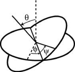
FIG. 1.: The Euler angles, $\theta$, $\phi$ and $\psi$.

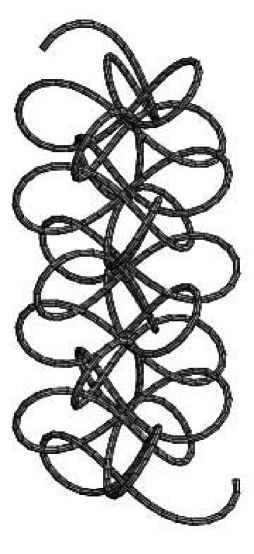
FIG. 2.: The solution to the equation that corresponds to the nucleosome configuration

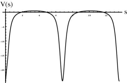
FIG. 3.: The effective potential, $V(s)$ in the operator in (9)

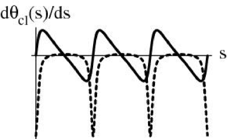
FIG. 4.: The translational mode, $d\theta_{\rm cl}(s)/ds$. Also shown, as a dashed curve, is the effective potential, $V(s)$, in the operator in (9).

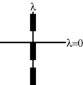
FIG. 5.: The spectrum of the potential shown in Figure 3

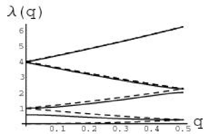
FIG. 6.: Alteration of the band structure as the result of a periodic array of constraints. The dotted curves are the bands in the absence of constraints. The solid curves represent the influence of constraints.

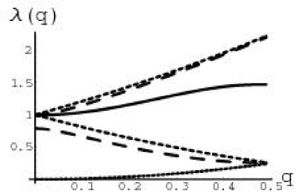
FIG. 7.: Alteration of the band structure as the result of a periodic array of constraints, when there are two constraints per period. Here the solid curve is the result for $\lambda(q)$ when there are two constraints per period. The dashed curve represents the influence of one constraint, and the dotted curves are the bands in the absence of constraints. The solid curves represent the influence of constraints.

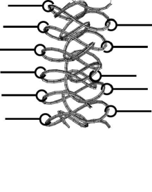
FIG. 8.: A schematic representation of a non-trivial supercoiled configuration of DNA stabilized by a protein armature.

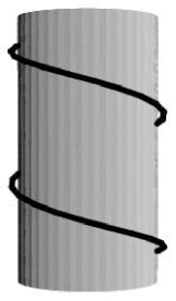
FIG. 9.: Schematic of the nucleosome.

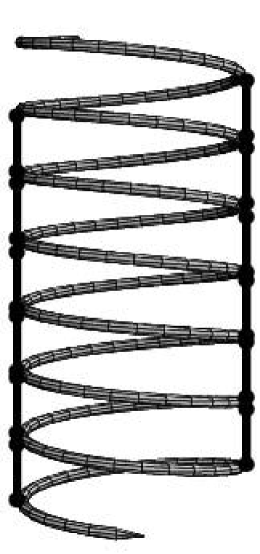
FIG. 10.: The constrained spiral

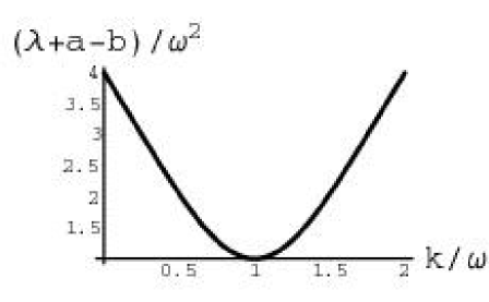
FIG. 11.: The eigenvalue of the constrained fluctuation operator in the case of interest here.

FIG. 12.: The portion of the compound spiral in Fig. 2 that corresponds to a nucleosome in the 30 nm spiral.

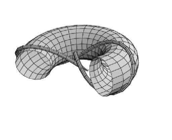
FIG. 13.: The nuclesome configuration in this case. Note the the “histone” is in the form of a curved cylinder. The curvature is so as to fit into the two-loop structure that we investigate here.

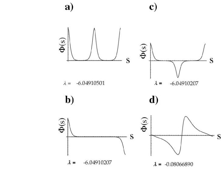
FIG. 14.: The four unstable eigenvalues of the fluctuation operator for the “nucleosome” configuration illustrated in Figure 13. The associated eigenvalues are shown immediately below the graphs.

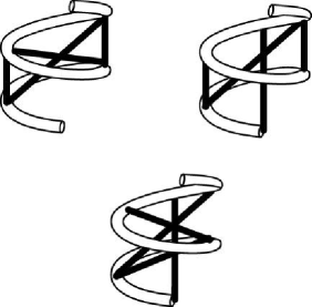
FIG. 15.: A figurative depiction of some of the constraints that were found to not stabilize the “nucleosome” configuration against fluctuations.

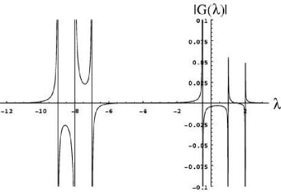
FIG. 16.: A determinant associated with one of the constraints that does not stabilize the nuclesome configuration illustrated in Figure 13. Note that this determinant passes through zero as a function of $\lambda$ for $\lambda<0$. Recall that zeros of the determinant are proportional to energy eigenvalues of the fluctuation operator.

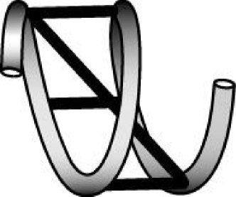
FIG. 17.: A figurative version of the actual set of constraints that were utilized in this set of calculations. In this picture, the “histone” has been straightened out to resemble a the cylindrical shape that it actually takes.

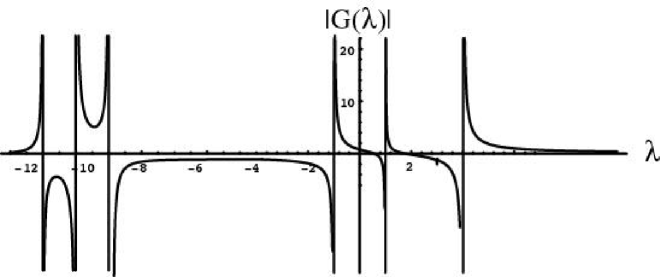
FIG. 18.: The determinant yielding the eigenvalues of the constrained fluctuation spectrum for the case of the constraints on the two loops in Figure 12 that are described in Section VIII. Note that this determinant as function of $\lambda$ does not pass through zero for any $\lambda<0$. Given that zeroes of the determinant are proportional to energy eigenvalues of the constrained fluctuation operator, we are assured that the nuclesome configuration is stabilized against mechanical fluctuations.

REFERENCES

- [1] R. D. Kornberg Annu. Rev. Biochem. 49, 115 (1977).
- [2] P. Oudet, M. Gross-Bellard, P. Chambon, Cell 4, 281 (1975).
- [3] K. Luger et. al. Nature 389, 251 (1997).
- [4] A. Klug et. al. Science 229, 1109 (1985).
- [5] T. J. Richmond et. al. Nature 311, 532 (1984).
- [6] A. Wolffe, Chromatin : structure and function (Academic Press, San Diego, 1998).
- [7] J. Bednar et. al. Proc. Nat. Acad. Sci. 95, 14173 (1998).
- [8] K. van Holde and J. Zlatanova, J. Biol. Chem. 8373 (1995).
- [9] J. L. Zlatanova, S. H., and K. van Holde, Crit. Rev. Eukaryotic Gene Expression 9, 245 (1999).
- [10] J. Widom, Annu. Rev. Biomol. Struct. 27, 285 (1998).
- [11] J. Kirchhoff, J. f. Math (Crelle) 56, (1859).
- [12] B. Y. Ha and A. J. Liu, Physical Review Letters 79, 1289 (1997).
- [13] C. J. Benham, Proc. Nat. Acad. Sci. 74, 2397 (1977).
- [14] A. E. H. Love, A Treatise on the Mathematical Theory of Elasticity (Dover, New York, 1944).
- [15] B. Fain, J. Rudnick and S. Östllund , Phys. Rev. E55 7364, (1997).
- [16] B. Fain and J. Rudnick, Phys. Rev. E 60, 7239 (1999).
- [17] S. Coleman Aspects of Symmetry (Cambridge University Press, 1985) p. 265-350.
- [18] J. O. Thomas and R. D. Kornberg, Proc. Natl. Acad. Sci. 72, 72 (1975).
- [19] G. Arents et. al., Proc. Natl. Acad. Sci. 88, 10148 (1991).
- [20] G. Arents and E. N. Moudrianakis, Proc. Natl. Acad. Sci. 90, 10489 (1993).
- [21] We are grateful to Prof. W. M. Gelbart for bringing this to our attention.
- [22] A. Klug, et. al., Nature 287, 509 (1980).