Macroscopic quantum tunneling of two-component Bose-Einstein condensates

Abstract

We show theoretically the existence of a metastable state and the possibility of decay to the ground state through macroscopic quantum tunneling in two-component Bose-Einstein condensates with repulsive interactions. Numerical analysis of the coupled Gross-Pitaevskii equations clarifies the metastable states whose configuration preserves or breaks the symmetry of the trapping potential, depending on the interspecies interaction and the particle number. We calculate the tunneling decay rate of the metastable state by using the collective coordinate method under the WKB approximation. Then the height of the energy barrier is estimated by the saddle point solution. It is found that macroscopic quantum tunneling is observable in a wide range of particle numbers. Macroscopic quantum coherence between two distinct states is discussed; this might give an additional coherent property of two-component Bose condensed systems. Thermal effects on the decay rate are estimated.

I INTRODUCTION

Multicomponent Bose-Einstein condensates (BECs) of alkali-metal atomic gases are expected to exhibit macroscopic quantum phenomena that have not been found in a single condensate. Multicomponent atomic gases can be obtained experimentally by trapping different atomic species or the same atoms with different hyperfine spin states. The experimental realization of multicomponent BECs Myatt ; Stenger ; Miesner further stimulated many researchers to study the physics of this interesting system.

Macroscopic quantum tunneling (MQT) is an interesting subject in many fields of physics. In this paper we study MQT of metastable two-component BECs in a trapping potential. Thus we need to know detailed information about the stationary state of this system. The structure of the ground state has been studied by solving two coupled Gross-Pitaevskii equations (GPEs) analytically or numerically Ho ; Ersy ; Pu ; Ohberg ; Bashkin ; Tim ; Ersy2 ; Ao ; Tr ; Tanatar ; Gordon ; Ohberg2 . The stationary solution of the GPEs gives the density profile of the condensate characterized by the parameters of the system—trapping frequencies, the number of atoms of each component, and three s-wave scattering lengths, $a_{1}$, $a_{2}$, and $a_{12}$, which represent the interactions between like and unlike components.

The interspecies interaction characterized by $a_{12}$ plays an important role in determining the structure of the ground state. When the inequality $a_{12}>\sqrt{a_{1}a_{2}}$ is satisfied, a mixture of two-component BECs without a trapping potential tends to separate spatially Tim ; Ao . The trapped BECs have two different configurations of the condensates when $a_{12}$ is large Ohberg ; Ersy2 . One configuration preserves the spatial symmetry of the trapping potential by forming a core-shell structure. The other breaks the spatial symmetry by displacing the center of each condensate from that of the trapping potential.

Ho and Shenoy first constructed a simple algorithm to determine the density profile within the Thomas-Fermi approximation (TFA) Ho . However, the TFA is not enough to describe the density profile of phase separation because the penetration at the boundary of each component is not considered. Without the TFA Pu and Bigelow investigated numerically the ground state of a Rb-Na BECs by assuming spherical symmetry Pu . When $a_{12}$ is large, they found a ground state that forms a core of Rb at the center of the trap and a shell of Na around Rb, and a metastable state that has a Rb shell and Na core. However, they noted the existence of an unstable mode which forms the core-shell structure. After that, further investigation of two- or three-dimensional GPEs showed a spherical symmetry-breaking solution for the true ground state Ohberg ; Ersy2 ; Gordon .

Öhberg showed that whether the ground state takes a symmetry-breaking state (SBS) or a symmetry-preserving state (SPS) depends not only on the interspecies interaction but also on the particle number, the intraspecies interaction, and the shape of the trapping potential Ohberg2 . However, the detaila of the metastable state have not been studied. Thus, we investigate the dependence of the ground state and the metastable state of two-component BECs in a cigar-shaped potential, which can be considered as a quasi-one-dimensional system for simplicity. We also make a linear stability analysis of the stationary solutions of the GPEs and reveal their metastability.

A metastable BEC can also be found in a single condensate with negative s-wave scattering length Bradley . The negative scattering length represents an attractive atom-atom interaction, which causes the condensate to collapse upon itself to a denser phase. The balance between the attractive interaction energy and the zero-point kinetic energy of the trapping potential realizes the metastable condensate. MQT of a condensate with attractive interaction has been predicted Ueda .

For two-component BECs with repulsive interactions the metastability mainly comes from the competition between intra- and interspecies interactions. We study the transition between the SBS and SPS by MQT.

In Sec. II, we obtain the stationary solution of the GPEs numerically. The phase diagram of the ground state has a rich structure including metastable states. The stability of these solutions is checked by following Ref. Law which considers the stability by taking account of the linear fluctuation around the stationary solution.

In Sec. III, we introduce the collective coordinate method to evaluate the decay rate of a metastable state through MQT by an imaginary-time path integral (instanton) technique. The collective coordinate enables us to derive an effective one-dimensional Lagrangian describing the two-component BECs and obtain the decay rate. We estimate the decay rate at finite temperatures; the results show the probability of observation of MQT. We also discuss macroscopic quantum coherence (MQC), which is the oscillation between the SPS and the SBS. Section IV is devoted to conclusions and discussion.

II FORMULATION AND STATIONARY SOLUTION

We consider two-component BECs in the external trapping potentials

$$V_{\text{ext}}^{i}({\bf r})=\frac{1}{2}m_{i}\omega_{i}^{2}x^{2}+\frac{1}{2}m_{i}\omega_{i\perp}^{2}(y^{2}+z^{2}),\hskip 8.53581pti=1,2,$$ (1)

where $m_{i}$ is the atomic mass, and $\omega_{i}$ and $\omega_{i\perp}$ are the longitudinal and transverse trapping frequencies. For $\omega_{i\perp}\gg\omega_{i}$ the trapping potential is cigar-shaped. If the two-body interaction energy is smaller than $\hbar\omega_{\perp}$, it does not affect the transverse component $\psi_{i\perp}$ of the wave functions, which allows us to analyze the problem in one-dimensional space. Although it has been predicted that the two-body interaction is changed by the effect of tight confinement of the trapping potential Olshanii ; Petrov , we will use the following treatment to derive the one-dimensional GPEs Goldstein . Using the ground state wave function in the harmonic potential for $\psi_{i\perp}(y,z)$, we assume the macroscopic wave function as $\Psi_{i}({\bf r},t)=\psi_{i}(x,t)\psi_{i\perp}(y,z)$ $(i=1,2)$. These wave functions are substituted into the three-dimensional Gross-Pitaevskii energy functional, which is integrated over $y$ and $z$. Thus we obtain the one-dimensional Gross-Pitaevskii energy functional,

$${\cal H}[\psi_{1},\psi_{2}] = \int dx\biggl{[}\sum_{i=1,2}\biggl{(}\frac{\hbar^{2}}{2m_{i}}\left|\frac{\partial\psi_{i}}{\partial x}\right|^{2}+\frac{1}{2}m_{i}w_{i}^{2}x^{2}|\psi_{i}|^{2}$$ (2)

$$-\mu_{i}|\psi_{i}|^{2}\biggr{)}+\frac{1}{2}U_{11}|\psi_{1}|^{4}+\frac{1}{2}U_{22}|\psi_{2}|^{4}$$

$$+U_{12}|\psi_{1}|^{2}|\psi_{2}|^{2}\biggr{]}$$

with the chemical potential $\mu_{i}$. Here the two-body interactions $U_{ii}$ and $U_{12}$ are written as

$$U_{ii} = g_{ii}\int dydz\left|\psi_{i\perp}(y,z)\right|^{4}=\frac{g_{ii}}{2\pi b_{i\perp}^{2}},$$ (3a)

$$U_{12} = g_{12}\int dydz\left|\psi_{1\perp}(y,z)\right|^{2}\left|\psi_{2\perp}(y,z)\right|^{2}$$ (3b)

$$= \frac{g_{12}}{\pi(b_{1\perp}^{2}+b_{2\perp}^{2})},$$

where $b_{i\perp}=\sqrt{\hbar/m_{i}\omega_{i\perp}}$, $g_{ii}=4\pi\hbar^{2}a_{i}/m_{i}$ and $g_{12}=2\pi\hbar^{2}a_{12}/m_{12}$ with reduced mass $m_{12}$. The corresponding two coupled time-dependent GPEs are given by

$$i\hbar\frac{\partial\psi_{i}}{\partial t}=H_{i}[\psi_{1},\psi_{2}]\psi_{i},$$ (4)

where

$$H_{1}[\psi_{1},\psi_{2}] = -\frac{\hbar^{2}}{2m_{1}}\frac{\partial^{2}}{\partial x^{2}}+\frac{1}{2}m_{1}\omega_{1}^{2}x^{2}-\mu_{1}$$ (5a)

$$+U_{11}|\psi_{1}|^{2}+U_{12}|\psi_{2}|^{2},$$

$$H_{2}[\psi_{1},\psi_{2}] = -\frac{\hbar^{2}}{2m_{2}}\frac{\partial^{2}}{\partial x^{2}}+\frac{1}{2}m_{2}\omega_{2}^{2}x^{2}-\mu_{2}$$ (5b)

$$+U_{22}|\psi_{2}|^{2}+U_{12}|\psi_{1}|^{2},$$

and each wave function is normalized by the number of particles $N_{i}$ as $\int dx|\psi_{i}(x)|^{2}=N_{i}$.

II.1 Numerical solution

The stationary solutions of Eq. (4) correspond to the critical points of the energy functional ${\cal H}$. There are several ways to find these critical points numerically. Our method is described in the following. The stationary solution $\psi_{i0}$ satisfies the relation

$$H_{i}[\psi_{10},\psi_{20}]\psi_{i0}=0$$ (6)

from Eq. (4). The solution $\psi_{i0}$ is taken to be real by making the phase zero. Using the trial function $\psi_{i}^{\text{tri}}$, $\psi_{i0}$ is given by $\psi_{i}^{\text{tri}}$ and its deviation $\Delta\psi_{i}$, i.e., $\psi_{i0}=\psi_{i}^{\text{tri}}-\Delta\psi_{i}$. Substituting this relation in Eq. (6), we obtain the linearized equation for $\Delta\psi_{i}$:

$${H_{1}[\psi_{1}^{\text{tri}},\psi_{2}^{\text{tri}}]+2U_{11}(\psi_{1}^{\text{tri}})^{2}}\Delta\psi_{1}$$

$$+2U_{12}\psi_{1}^{\text{tri}}\psi_{2}^{\text{tri}}\Delta\psi_{2}=\sigma_{1},$$ (7a)

$${H_{2}[\psi_{1}^{\text{tri}},\psi_{2}^{\text{tri}}]+2U_{22}(\psi_{2}^{\text{tri}})^{2}}\Delta\psi_{2}$$

$$+2U_{12}\psi_{1}^{\text{tri}}\psi_{2}^{\text{tri}}\Delta\psi_{1}=\sigma_{2},$$ (7b)

where $\sigma_{i}=H_{i}[\psi_{1}^{\text{tri}},\psi_{2}^{\text{tri}}]\psi_{i}^{\text{tri}}$. The linear correction $\Delta\psi_{i}$ can easily be calculated and the modified trial function is defined by $\psi_{i}=\psi_{i}^{\text{tri}}-\Delta\psi_{i}$. We repeat the above calculation until the solution converges by conserving the norm of each component.

Assuming the condensates of two hyperfine spin states of ⁸⁷Rb, we use the values of the scattering lengths $a_{1}=5.36$ nm and $a_{2}=5.66$ nm, which have the ratio $a_{2}/a_{1}=1.06$ Matthews . We choose the atomic mass $m_{1}=m_{2}=m_{\text{Rb}}=1.45\times 10^{-25}$ kg, the trapping frequency $\omega_{1}=\omega_{2}=\omega=90\times 2\pi$ Hz, and the aspect ratio $\omega_{\perp}/\omega=30$. It is convenient to introduce scales characterizing the trapping potential: (a) the length scale $b=\sqrt{\hbar/m_{12}\omega}$, (b) the time scale $\omega^{-1}$, and (c) the energy scale $\hbar\omega$. The dimensionless parameters normalized by these scales are expressed by putting a tilde upon the symbols. Then the dimensionless intraspecies interactions become $\tilde{U}_{11}=0.2010$ and $\tilde{U}_{22}=0.2123$ from Eqs. (3). Setting the particle numbers to $N_{1}=N_{2}=N$ for simplicity, our formulation has two free parameters, $N$ and $\tilde{U}_{12}$. The parameter $\tilde{U}_{12}$ might be controlled experimentally by the choice of some combination of atoms, or by changing the scattering length via the Feshbach resonance Inouye .

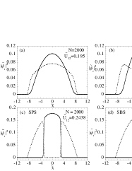
Figure 1: Numerical solutions of the two coupled stationary GPEs. The solid lines and the dotted lines show the condensates 1 and 2, respectively. The wave functions $\tilde{\psi}_{i}$ divided by $\sqrt{N}$ and the coordinate $\tilde{x}$ are normalized by the length scale $b=\sqrt{\hbar/m_{12}\omega}$. (c) shows the symmetry-preserving state with energy 87.4261 in units of $\hbar\omega N$. (d) shows the symmetry-breaking state with energy 87.5514.

Typical stationary solutions of Eq. (4) are shown in Fig. 1. When the interspecies interaction is weak, two condensates overlap each other. For $\tilde{U}_{12}<\tilde{U}_{11}<\tilde{U}_{22}$ two overlapping condensates have peaks of the density at the center of the trapping potential, as shown in Fig. 1(a). For $\tilde{U}_{11}<\tilde{U}_{12}<\tilde{U}_{22}$ and $\sqrt{\tilde{U}_{11}\tilde{U}_{22}}<\tilde{U}_{12}$, the density peak of condensate 2 is not at the center and two peaks appear symmetrically about the origin $\tilde{x}=0$, as shown in Fig. 1(b). Note that the width of condensate 2 is larger than that of 1, because $\tilde{U}_{11}<\tilde{U}_{22}$. These structures can be predicted easily within the TFA Ho ; Tr . For $\tilde{U}_{12}>\sqrt{\tilde{U}_{11}\tilde{U}_{22}}$ the two condensates separate from each other with very narrow overlapping regions. In Fig. 1(c) the condensate 1 occupies the central region, pushing aside the condensate 2 symmetrically; this configuration preserves the spatial symmetry of the trapping potential. On the other hand, as shown in Fig. 1(d), there exists another configuration with the boundary between the two condensates at the center of the trapping potential and its spatial symmetry is broken. Now we call the stationary state in Fig. 1(c) the symmetry-preserving state and that in Fig. 1(d) the symmetry-breaking state. The total energy of solution (c) is lower than that of (d) as described in the figure caption, so that the solution (d) represents the metastable state.

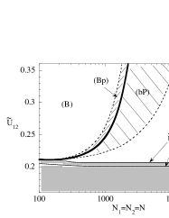
Figure 2: $N$-$\tilde{U}_{12}$ phase diagram of the ground state. The gray region represents the overlapping configuration and the other the separated configuration. In region $B$ the SBS is the ground state, while in region $P$ the SPS is the ground state. In the region with slanted lines, there exists the metastable SBS (SPS) denoted by the lower-case letter $b$($p$).

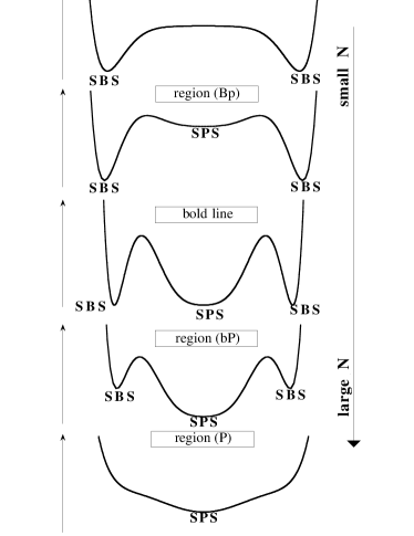
Figure 3: Schematic illustration of the total energy in the region of the separated configurations in Fig. 2. When the energy of the SBS is equal to that of the SPS, the energy configuration becomes a triple well.

In Fig. 2 we show the $N$-$\tilde{U}_{12}$ phase diagram of the ground state. The gray region represents the overlapping configurations, Fig. 1(a) and 1(b), and the other the separated configurations, Fig. 1(c) and 1(d); the two regions are divided by the line $\tilde{U}_{12}=\sqrt{\tilde{U}_{11}\tilde{U}_{22}}=0.2066$ which was predicted by the TFA Ersy ; Bashkin ; Tim ; Ersy2 ; Ao ; Tr . The gray region is further divided into two regions [Fig. 1(a) and 1(b)] by the line $\tilde{U}_{12}=0.2010$ Tr . More precisely, these boundaries are bent for small $N$ because of the failure of the TFA. The region of the separated configurations has the following structure. The bold line shows the boundary where the energy of the SBS is equal to that of the SPS. In region $B$ the SBS is the ground state, while in region $P$ the SPS is the ground state.

The position of the SBS and the SPS in the phase diagram Fig. 2 can be understood as follows. We first consider the transition on increasing the particle number $N$ with a fixed value of $\tilde{U}_{12}$. Note that the SBS has one domain wall and the SPS two domain walls. When $N$ is small, the SBS is realized because the multiple domain walls increase the domain wall energy, which is estimated by the energy $\int dx[\sum_{i}(\hbar^{2}/2m_{i})|\nabla\psi_{i}|^{2}+U_{12}|\psi_{1}|^{2}|\psi_{2}|^{2}]$ in Eq. (2). The increase in $N$ makes the intraspecies interaction energy important, thus tending to extend each domain. This overcomes the energy of formation of domain walls, so that the SPS becomes more stable than the SBS. When $\tilde{U}_{12}$ increases, the domain wall energy becomes larger and thus the region $B$ is extended.

The bold line suggests the existence of metastable states as shown in Fig. 3. In Fig. 2, the regions $Bp$ and $bP$ have metastable states; the SBS is the ground state and the SPS is the metastable state in the region $Bp$, and vice versa in the region $bP$. The details of the metastable state and how to decide the boundaries between $B$ and $Bp$, $bP$ and $P$ are described in the next subsection.

II.2 Stability of the solutions

We linearize the energy functional ${\cal H}$ of Eq. (2) by substituting

$$\psi_{i}=\psi_{i0}+\delta\psi_{i}.$$ (8)

Here $\psi_{i0}$ is the stationary solution obtained by solving the GPEs, and the fluctuation $\delta\psi_{i}$ is complex. The stationary solutions represent the local minima or the saddle points of the energy functional. Then the energy can be expanded around the stationary solution:

$${\cal H}[\psi_{1},\psi_{2}] \simeq {\cal H}_{0}+\delta{\cal H}[\delta\psi_{1},\delta\psi_{2}],$$ (9)

$$\delta{\cal H}[\delta\psi_{1},\delta\psi_{2}] = \frac{1}{2}\sum_{i,j=1}^{4}\int d{\bf r}\eta_{i}W_{ij}\eta_{j}.$$ (10)

Here ${\bf\eta}=(\eta_{1},\eta_{2},\eta_{3},\eta_{4})\equiv(\delta\psi_{1},\delta\psi_{2},\delta\psi_{1}^{\ast},\delta\psi_{2}^{\ast})$ and $W=(W_{ij})$ is the Hessian operator, corresponding to the second-order derivative of the energy functional at the stationary solution:

$$W_{11} = W_{33}=-\frac{\hbar^{2}}{2m_{1}}\frac{\partial^{2}}{\partial x^{2}}+\frac{1}{2}m_{1}\omega_{1}^{2}x^{2}-\mu_{1}$$

$$\hskip 28.45274pt+2U_{11}\psi_{10}^{2}+U_{12}\psi_{20}^{2},$$

$$W_{22} = W_{44}=-\frac{\hbar^{2}}{2m_{2}}\frac{\partial^{2}}{\partial x^{2}}+\frac{1}{2}m_{2}\omega_{2}^{2}x^{2}-\mu_{2}$$

$$\hskip 28.45274pt+2U_{22}\psi_{20}^{2}+U_{12}\psi_{10}^{2},$$

$$W_{12} = W_{23}=W_{34}=W_{41}=U_{12}\psi_{10}\psi_{20},$$

$$W_{13} = U_{11}\psi_{10}^{2},\hskip 22.76219ptW_{24}=U_{22}\psi_{20}^{2}.$$

When all eigenvalues of $W$ are positive, the stationary solution is stable, while the appearance of a negative eigenvalue makes it unstable.

This eigenvalue problem is simplified by the unitary transformation Law

$$U^{\dagger}WU=\left(\begin{array}[]{ccc}L_{1}&0\\ 0&L_{2}\end{array}\right),$$ (11)

where

$$L_{1} = \left(\begin{array}[]{ccc}W_{11}-U_{11}\psi_{10}^{2}&0\\ 0&W_{22}-U_{22}\psi_{20}^{2}\end{array}\right),$$ (14)

$$L_{2} = \left(\begin{array}[]{ccc}W_{11}+U_{11}\psi_{10}^{2}&2W_{12}\\ 2W_{21}&W_{22}+U_{22}\psi_{20}^{2}\end{array}\right),$$ (17)

and

$$U = \left(\begin{array}[]{ccc}{\bf a}&{\bf b}\\ -{\bf a}&{\bf b}\end{array}\right),$$ (20)

$${\bf a}=\left(\begin{array}[]{ccc}a&0\\ 0&a\end{array}\right),\hskip 5.69054pt{\bf b} = \left(\begin{array}[]{ccc}b&0\\ 0&b\end{array}\right),\hskip 5.69054pt|a|^{2}=|b|^{2}=\frac{1}{2}.$$ (25)

Law et al. used the lowest eigenvalue of $L_{2}$ as the stability criterion of the system of two-component BECs Law . The lowest eigenvalue of $L_{1}$ is zero and the eigenfunction is given by the stationary solution $\psi_{i0}$.

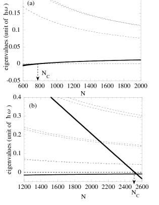
Figure 4: Several lower eigenvalues of $W$ for the SPS (a) and the SBS (b). The bold lines show the eigenvalues of $L_{2}$ and the dashed lines show those of $L_{1}$. The critical particle number is represented by $N_{c}$.

Figure 4 shows several lower eigenvalues of $W$ as functions of $N$ for the SPS (a) and SBS (b) with $\tilde{U}_{12}=0.2438$ as used in Fig. 1(c) and 1(d). The critical particle number $N_{c}$ defined by the zero eigenvalue of $L_{2}$ gives the criterion for the stability of the stationary solution. From Fig. 4(a), the SPS is stable for $N>N_{c}$. Figure 4(b) shows that there always exists one negative eigenvalue whose eigenfunction changes $N$. Hence, as long as $N$ is fixed, the SBS is stable for $N<N_{c}$. Obtaining $N_{c}$ as a function of $\tilde{U}_{12}$ allows us to decide the boundaries between the regions $B$ and $Bp$, $P$ and $bP$ in Fig. 2.

Finally, let us note the fluctuation changing the particle number. By using the eigenfunction ${\bf u}=(u_{1},u_{2})$ of $L_{2}$ this fluctuation is evaluated as

$$\delta N_{i}\simeq 2\int\psi_{i0}(x)u_{i}(x)dx.$$ (26)

For the mode in Fig. 4(b) whose eigenvalue is always negative we obtain $\delta N_{i}\neq 0$. The other mode of $L_{2}$ in Fig. 4(b) conserves the particle number. The fluctuation that changes the particle number leads to the ground state of the SBS with unbalanced particle number $N_{1}\neq N_{2}$ Law .

III POSSIBILITY OF MACROSCOPIC QUANTUM TUNNELING

As described in Sec. II, the SBS is the ground state and the SPS is the metastable state in the region $Bp$ in Fig. 2, and vice versa in the region $bP$. In this section, we study the MQT of the metastable state in $Bp$ and $bP$.

III.1 Collective coordinate approach

It is difficult to consider MQT by full quantum field theory. In the case of a single condensate, the variational method is often used to estimate the condensate wave function. This method was applied to the evaluation of the decay rate via MQT of a metastable condensate with attractive interaction Ueda . However, there is an important difference in the description of the decay of a single condensate and the transition between the SBS and SPS in two-component condensates. In the former case, there is an obvious collective coordinate, i.e., the spatial size of the condensate wave function, which allows us to approximate the wave function under the Gaussian ansatz Ueda . In contrast, in the latter case, it is difficult to find suitable collective coordinates that can describe the continuous deformation from a metastable state to the ground state. Thus we introduce an alternative variational approach for this system in order to calculate the MQT rate.

The action $S$ for the Gross-Pitaevskii model is given by $S=\int{\cal L}dt$ with the Lagrangian

$${\cal L}=\sum_{i=1,2}\int dx\left(i\hbar\psi_{i}^{\ast}\frac{\partial}{\partial t}\psi_{i}\right)-{\cal H},$$ (27)

where ${\cal H}$ is the Hamiltonian of Eq. (2). The macroscopic wave functions are written as $\psi_{i}=\Phi_{i}(x,t)e^{i\theta_{i}(x,t)}$, where $\Phi_{i}^{2}=\rho_{i}$ and $\theta_{i}$ are the number density and the phase for each component, respectively. Substituting these forms in Eq. (27) yields

$${\cal L}=\int dx\left[\sum_{i=1,2}\left\{\hbar\frac{\partial\rho_{i}}{\partial t}\theta_{i}-\frac{\hbar^{2}}{2m_{i}}\Phi_{i}^{2}\left(\frac{\partial\theta_{i}}{\partial x}\right)^{2}\right\}-V(\Phi_{i})\right],$$ (28)

where $V(\Phi_{i})$ is written as

$$V(\Phi_{i}) = \sum_{i=1,2}\left[\frac{\hbar^{2}}{2m_{i}}\left(\frac{\partial\Phi_{i}}{\partial x}\right)^{2}+(V_{\text{ext}}^{i}-\mu_{i})\Phi_{i}^{2}\right]$$ (29)

$$+\frac{U_{11}}{2}\Phi_{1}^{4}+\frac{U_{22}}{2}\Phi_{2}^{4}+U_{12}\Phi_{1}^{2}\Phi_{2}^{2}.$$

The amplitude $\Phi_{i}$ can be expanded around the stationary solution $\Phi_{i}^{s}=\sqrt{\rho_{i}^{s}}=|\psi_{i0}|$ in Sec. II by using an orthogonal complete set $u_{in}(x)$,

$$\Phi_{i}(x,t)=\Phi_{i}^{s}(x)+\sum_{n}\tilde{Q}_{n}(t)u_{in}(x)\hskip 14.22636pt(n=1,2,...),$$ (30)

with the normalization

$$\sum_{i=1,2}\int u_{in}u_{im}dx=\delta_{nm}.$$ (31)

Here $\tilde{Q}_{n}(t)$ stands for the dimensionless arbitrary function and represents the small displacement of the density profile from the stationary solution:

$$\sum_{n}\tilde{Q}_{n}^{2}(t)=\sum_{i=1,2}\int dx\left[\Phi_{i}(x,t)-\Phi_{i}^{s}(x)\right]^{2}$$ (32)

$$(n=1,2,...).$$

Substituting Eq. (30) to Eq. (28), we can obtain the effective action written by the functions $\tilde{Q}_{n}(t)$. If we assume that the phase has the form $\theta_{i}(x,t)=\sum_{n}\tilde{P}_{n}(t)v_{in}(x)/N$ with some complete set $v_{in}(x)$, the first term of Eq. (28) can be written as

$$\sum_{nm}2\hbar\frac{\tilde{P}_{m}(t)}{N}\dot{\tilde{Q}}_{n}(t)\sum_{i}\int dxv_{im}(x)\Phi_{i}^{s}(x)u_{in}(x),$$ (33)

by using $\dot{\rho}_{i}\simeq 2\sum_{n}\dot{\tilde{Q}}_{n}\Phi_{i}^{s}u_{in}$. Then we define the collective coordinate $Q_{n}=b\tilde{Q}_{n}/\sqrt{N}$ and the collective momentum $P_{m}=2\hbar\tilde{P}_{m}/b$ with the length scale $b$ of the trapping potential. By choosing the complete set $v_{in}(x)$ as

$$\sum_{i}\int dxv_{im}(x)\frac{\Phi_{i}^{s}(x)}{\sqrt{N}}u_{in}(x)=\delta_{mn},$$ (34)

the first term of Eq. (28) becomes $\sum_{n}P_{n}\dot{Q}_{n}$ and the second term

$$\int dt\sum_{mn}\frac{P_{m}(t)P_{n}(t)}{2M_{mn}},$$ (35)

where the effective mass matrix $M_{mn}$ is given by

$$\frac{1}{M_{mn}}=\sum_{i=1,2}\frac{b^{2}}{4m_{i}N^{2}}\int\rho_{i}^{s}\left(\frac{dv_{im}}{dx}\frac{dv_{in}}{dx}\right)dx.$$ (36)

The potential $V(\Phi_{i})$ is a function of the collective coordinate $Q_{n}$. Thus we can obtain the effective action

$$S\simeq\int dt\left[\sum_{n}P_{n}\dot{Q}_{n}-{\cal H}_{\text{eff}}({\bf P},{\bf Q})\right],$$ (37)

$${\bf P}=(P_{1},P_{2},...),\hskip 8.53581pt{\bf Q}=(Q_{1},Q_{2},...),$$

with the effective Hamiltonian

$${\cal H}_{\text{eff}}({\bf P},{\bf Q})=\sum_{mn}\frac{P_{m}P_{n}}{2M_{mn}}+V({\bf Q}).$$ (38)

By substituting Eq. (30) into Eq. (29) the effective potential $V({\bf Q})$ can be expanded as follows:

$$V({\bf Q})=\int V(\Phi_{i}^{s})dx+\frac{1}{2}\sum_{n}\tilde{Q}_{n}^{2}\sum_{i,j}u_{in}H_{ij}u_{jn}+\cdot\cdot\cdot.$$ (39)

Here the linear term in $Q_{n}$ vanishes because $\Phi_{i}^{s}$ is the stationary solution. The quadratic term of $Q_{n}$ can be written by the Hessian operator $H_{ij}$, which is equal to $2L_{2}$ given by Eq. (17). We take the orthogonal set $u_{in}$ as the eigenfunction of $L_{2}$. Thus the second term of Eq. (39) is diagonalized and $V({\bf Q})$ is written as

$$V({\bf Q})=\int V(\Phi_{i}^{s})dx+\frac{1}{2}\sum_{n}N\lambda_{n}^{2}\frac{Q_{n}^{2}}{b^{2}}+\cdot\cdot\cdot,$$ (40)

where $\lambda_{n}^{2}$ $(n=1,2,...)$ are the eigenvalues of $H_{ij}$. The constant $\int V(\Phi_{i}^{s})dx$ will be chosen to be zero in the following section.

III.2 Calculation of the decay rate

We now calculate the MQT rate $\Gamma$ of the metastable state in Fig. 2. The energy of the metastable state must have an (exponentially small) imaginary part when the tunneling is taken into account. Then the decay rate of the metastable state is given by Kleinert

$$\Gamma=\frac{2}{\hbar}\text{Im}E_{g}.$$ (41)

The energy $E_{g}$ is evaluated by the partition function

$$Z(\beta)\equiv e^{-W(\beta)}={\rm tr}(e^{-\beta H})$$ (42)

as

$$E_{g}=\lim_{\beta\rightarrow\infty}\frac{W(\beta)}{\beta},$$ (43)

where $\beta=1/k_{B}T$. Using the action Eq. (37) with the imaginary time $t\rightarrow-i\tau$ (Euclidean action $S_{E}$), the partition function is written as

$$Z(\beta)=\int D{\bf Q}(\tau)\exp\left[-\frac{S_{E}({\bf Q})}{\hbar}\right].$$ (44)

Within the WKB approximation this path integral is evaluated by the saddle-point method Kleinert . More precisely, the dominant contributions to the path integral are from paths that minimize the Euclidean action $S_{E}$. Such paths are the solution of the Euler-Lagrange equation $\delta S_{E}/\delta{\bf Q}=0$, the classical equation of motion for the valuables ${\bf Q}(\tau)$ in the inverted potential $-V({\bf Q})$. We choose the boundary condition that ${\bf Q(\tau)}$ approaches the metastable minimum at $\tau=\pm\infty$. By solving this equation of motion, we obtain the solution ${\bf Q}_{B}$ called the “bounce solution.” Then the decay rate has the form

$$\Gamma\simeq A\exp{\left(-\frac{S_{B}}{\hbar}\right)},$$ (45)

where $S_{B}=S_{E}({\bf Q}_{B})$ is the Euclidean action evaluated at the bounce solution ${\bf Q}_{B}$ and $A$ the quadratic quantum fluctuation around the bounce solution. The following describes how to approximate the bounce solution.

We are interested in the regions $Bp$ and $bP$ near the dashed lines in Fig. 2. These regions have metastable states as described in Sec. II. On the dashed lines, one of the eigenvalues of the Hessian operator $H_{ij}$ vanishes. Thus, in the region close to the dashed lines, the potential barrier of the metastable state is very small along the direction of the eigenfunction with the zero eigenvalue. We may assume that the direction of the initial (infinitesimal) velocity of the bounce solution is given by the eigenfunction ${\bf u}_{1}$ subject to the following conditions. First, ${\bf u}_{1}$ has the eigenvalue $\lambda_{1}^{2}$ which is small in this region and becomes zero on the dashed line. Secondly, this eigenfunction conserves the particle number, i.e., $\delta N_{i}=0$ in the sense of Eq. (26). Thus the trajectory of the bounce solution is mainly described by the collective coordinate $Q_{1}(t)$, which is the coordinate along the direction of ${\bf u}_{1}$, and the other coordinates $Q_{2}(t),Q_{3}(t),$ . . . give higher order corrections of the solution. These assumptions allow us to solve the bounce solution approximately; the trajectory of the bounce solution is straight in the collective coordinate space ${\bf Q}=(Q_{1},Q_{2},Q_{3}$. . . ) Yasui2 . Thus the infinite-dimensional system of Eq. (37) is reduced to a one-dimensional quantum mechanical system with the collective coordinate $Q_{1}$ subject to the action

$$S\simeq\int_{-\infty}^{\infty}dt\left[\frac{M}{2}\left(\frac{dQ_{1}}{dt}\right)^{2}+V(Q_{1})\right].$$ (46)

Here we have defined the mass $M$ by the (1,1) component of Eq. (36); the other components represent the mass relevant to $Q_{2},Q_{3}$ . . . , so that they are negligible. The mass $M$ includes unknown functions $v_{i1}$, although they satisfy Eq. (34). We will assume $v_{i1}\sim O(1)$, thus obtaining $M=M_{11}\sim(4m_{Rb}N^{2}/b^{2})\times(b^{2}/N)\sim m_{Rb}N$.

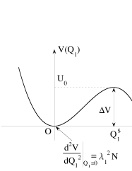
Figure 5: The quadratic-plus-cubic potential given by Eq. (47). The potential has a metastable minimum at $Q_{1}=0$, barrier height $U_{0}=\Delta V$ at $Q_{1}=Q_{1}^{s}$, and width $R_{0}$. The second derivative of $V(Q_{1})$ at $Q_{1}=0$ is given by $\lambda^{2}_{1}N$. The coordinate $Q_{1}^{s}$ corresponds to the sphaleron with energy $\Delta V$.

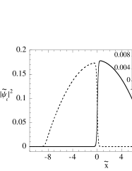
Figure 6: Saddle-point solution (sphaleron) of the two coupled stationary GPEs for $\tilde{U}_{12}=0.2438$ and $N=2000$. The unit of length is the same as in Fig.1. The inset shows the detail near $\tilde{x}=8$.

The next problem is to decide the form of the effective potential $V(Q_{1})$. It should be noticed the potential is expressed as $V(Q_{1})\simeq\frac{1}{2}N\lambda_{1}^{2}(Q_{1}^{2}/b^{2})$ for small $Q_{1}$ around the metastable state, from Eq. (40). As $Q_{1}$ increases, it is not clear how to extrapolate the potential. However, $V(Q_{1})$ should reflect the structure of the original potential $V(\Phi_{i})$ of Eq. (29), which has a metastable state in addition to the ground state as discussed in Sec. II. Hence we require, first, that $V(Q_{1})$ has a metastable minimum at $Q_{1}=0$. Secondly, as $Q_{1}$ increase, $V(Q_{1})$ increases once and decreases via a potential barrier $\Delta V$ as shown in Fig. 5. The potential is expected to be written as a power series of $Q_{1}$. Since the calculation of the decay rate does not need information on the ground state, we neglect the $n$th order terms ($n\geq 4$) and approximate the potential as

$$V(Q_{1})\simeq\frac{1}{2}N\lambda^{2}_{1}\frac{Q_{1}^{2}}{b^{2}}-\frac{1}{6}\alpha Q_{1}^{3}\hskip 8.53581pt(\alpha>0),$$ (47)

with an unknown parameter $\alpha$. Then the height of the potential barrier is given by

$$\Delta V=\frac{2N^{3}\lambda_{1}^{6}}{3\alpha^{2}b^{6}}.$$ (48)

The value of $\Delta V$ cannot be determined within the collective coordinate method. The barrier $\Delta V$ may be interpreted as follows. In general, when we consider quantum tunneling, it is natural to assume that the bounce trajectory will go through the sphaleron, which is the unstable stationary solution of the equation of motion, corresponding to the saddle point of the potential Manton . Then $\Delta V$ represents the energy of the sphaleron. In our case, the equation of motion is the GPE of the potential Eq. (29); we have found the sphaleron by numerical simulations (see Fig. 6) and obtained the value of $\Delta V$. The collective coordinate $Q_{1}$ of the sphaleron is simply written as

$$Q_{1}^{s}=2b\sqrt{\frac{3\Delta V}{2\lambda_{1}^{2}N}}.$$ (49)

Thus our collective coordinate $Q_{1}$ effectively describe MQT: the points $Q_{1}=0$ and $Q_{1}=Q_{1}^{s}$ correspond to the metastable state and the sphaleron, respectively, and the tunneling is represented by the bounce solution, going through the sphaleron. We will give the explicit bounce solution written via the collective coordinate in Eq. (56).

To calculate the decay rate of Eq. (45), it is convenient to introduce new scales characterizing the quantum tunneling instead of the scales of the trapping potential: according to Fig. 5 we define the length scale

$$R_{0}=3b\sqrt{\frac{3\Delta V}{2\lambda^{2}_{1}N}},$$ (50)

the energy scale

$$U_{0}=\Delta V,$$ (51)

and a time scale representing the “tunneling time”

$$\tau_{0}=R_{0}\sqrt{\frac{M}{U_{0}}}=\omega_{0}\sqrt{\frac{\hbar}{\omega\lambda^{2}_{1}}}\sqrt{\frac{M}{m_{12}N}}$$ (52)

with $\omega_{0}=\sqrt{27/2}.$ In these units the action Eq. (46) can be written by the dimensionless length $q=Q_{1}/R_{0}$ and the time $s=t/\tau_{0}$ as

$$\frac{S}{\hbar} = \frac{1}{h}\int_{-\infty}^{\infty}ds\left[\frac{1}{2}\left(\frac{dq}{ds}\right)^{2}+\tilde{V}(q)\right],$$ (53)

$$\tilde{V}(q) = \frac{1}{2}\omega_{0}^{2}q^{2}(1-q).$$ (54)

Here $h$ is the effective Planck constant defined as

$$h=\frac{\hbar}{\tau_{0}U_{0}}=\frac{1}{\omega_{0}}\sqrt{\frac{m_{12}N}{M}}\frac{\sqrt{\hbar\omega\lambda^{2}_{1}}}{\Delta V},$$ (55)

whose value must be smaller than unity for use of the WKB approximation, although it includes the macroscopic valuable $N$. From Eq. (53) the bounce solution can easily be obtained by solving the equation of motion $d^{2}q/ds^{2}=d\tilde{V}(q)/dq$ with the boundary condition $q=0$ at $s=\pm\infty$:

$$q_{B}(s)={\text{sech}}^{2}\left(\frac{\omega_{0}s}{2}\right),$$ (56)

and the decay rate can be written as

$$\Gamma\simeq\frac{\tilde{A}}{\tau_{0}}\exp\left(-\frac{\tilde{S}_{B}}{h}\right)$$ (57)

with the prefactor $\tilde{A}=4\sqrt{\omega_{0}^{3}/\pi h}$ and the bounce action $\tilde{S}_{B}=8\omega_{0}/15$.

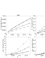
Figure 7: $\delta$ dependence of the eigenvalue $\lambda^{2}_{1}$ and the potential barrier $\Delta V$. The metastable SPS is shown in the left column and the metastable SBS in the right column. The open circles represent the numerical results of $\lambda_{1}^{2}$ and $\Delta V$ from the GPEs. The solid, dashed-dotted, and dotted lines show the scaling laws for $\tilde{U}_{12}=0.2250,0.2483,$ and $0.2813$, respectively.

We may observe MQT experimentally if the decay rate $\Gamma$ is of the order of the lifetime of the BEC. Let us search the region near the dashed lines in Fig.2 satisfying this condition. We obtained the potential barrier $\Delta V$ from the sphaleron energy and the eigenvalue $\lambda_{1}^{2}$ from the Hessian operator $H_{ij}$ . Recalling that $N$ is equal to the critical particle number $N_{c}$ on the dashed line (Sec. II.2), it is convenient to introduce a small parameter $\delta=|1-N/N_{c}|$. Figure 7 shows the $\delta$ dependence of $\lambda_{1}^{2}$ and $\Delta V$ for the metastable SPS and SBS near the dashed lines in Fig. 2. Since $\lambda_{1}^{2}$ and $\Delta V$ vanish on the dashed line with $\delta=0$, the scaling laws for the particle number are expected to be like those of a single condensate Ueda :

$$\lambda^{2}_{1} \simeq \hbar\omega{\cal C}\delta^{\beta},$$ (58)

$$\Delta V \simeq \hbar\omega{\cal D}\delta^{\gamma}.$$ (59)

The exponents $\beta$,$\gamma$ and the coefficients ${\cal C}$,${\cal D}$ are determined by fitting the scaling laws to the numerical results. Thus we obtain the exponents $\beta=1.0\pm 0.002$, $\gamma=2.06\pm 0.03$ for the metastable SBS, and $\beta=0.788\pm 0.006$, $\gamma=1.673\pm 0.007$ for the metastable SPS. As shown in Table. 1, they are approximately independent of the value of $U_{12}$ within our analysis, while the coefficients ${\cal C}$ and ${\cal D}$ depend on $U_{12}$. When we calculate $R_{0}$ and $U_{0}$ of Eqs. (50) and (51) by using these exponents and coefficients, we find that the metastable SPS has larger values of $R_{0}$ and $U_{0}$ than the SBS. Thus MQT cannot be expected for the metastable SPS compared with the metastable SBS.

Substituting Eq. (58) and Eq. (59) to $\tau_{0}$ and $h$ of Eqs. (52) and (55), we can obtain the scaling laws of the decay rate $\Gamma$ of Eq. (57) by

$$\frac{\tilde{S}_{B}}{h}\simeq\frac{8\omega_{0}^{2}}{15}\sqrt{\frac{M}{m_{12}N}}\frac{{\cal D}}{\sqrt{{\cal C}}}\delta^{\gamma-\beta/2},$$ (60)

and

$$\frac{\tilde{A}}{\tau_{0}}\simeq\omega\frac{4\omega_{0}}{\sqrt{\pi}}\left(\frac{M}{m_{12}N}\right)^{1/4}({\cal C}{\cal D}^{2})^{1/4}\delta^{\beta/4+\gamma/2}.$$ (61)

Table 1: The values ${\cal C,D},\beta,and\gamma$ of Eqs. (58) and (59).

metastable SPS

$\tilde{U}_{12}$	0.2250	0.2483	0.2813
${\cal C}$	0.03041	0.021508	0.015738
${\cal D}$	57.155	139.87	279.79
$\beta$	0.78718	0.79373	0.79177
$\gamma$	1.6684	1.6801	1.671

metastable SBS

$\tilde{U}_{12}$	0.2250	0.2483	0.2813
${\cal C}$	1.1445	2.0161	3.5006
${\cal D}$	17.454	20.462	26.086
$\beta$	1.0034	1.0022	1.0055
$\gamma$	2.068	2.0371	2.0562

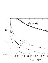
Figure 8: The solid lines show the effective Planck constant of the metastable SBS and the dashed lines show that of the metastable SPS. The parameter $\tilde{U}_{12}$ is set as 0.2250 for (a) and (d), 0.2438 for (b) and (e), and 0.2813 for (c) and (f). The critical particle number $N_{c}$ is (a) 481, (b) 770, (c) 1197, (d) 1121, (e) 2520, and (f) 5575. In the region $h>1$, the WKB approximation breaks down.

The dominant contribution to $\Gamma$ is the exponential factor. To obtain the observable decay rate, we require $h\sim 10^{-1}$, although $h$ should be small under the WKB approximation. Figure 8 shows the effective Planck constant for several values of $\tilde{U}_{12}$ as a function of $\delta=|1-N/N_{c}|$. The SBS has a wider range with respect to $\delta$ satisfying the above condition for $h$ than the SPS. Although it is difficult to tune the value of $\delta$ experimentally, we may observe MQT of the SBS more easily than that of the SPS. We now estimate the range of $\delta$ for $U_{12}=0.2483$ where $\Gamma$ becomes of the order of $10^{-2}$ sec^-1; the lifetime of the BEC is typically $100$ sec Myatt . The metastable SPS ($N_{c}=770$) yields $\tilde{S}_{B}/h=9713\times\delta^{1.283}$ and $\tilde{A}/\tau_{0}=44.66\times\omega\times\delta^{1.039}$ sec^-1, so that $\delta<3.9\times 10^{-3}$, a range too narrow to observe MQT. For the metastable SBS ($N_{c}=2520$) we obtain $\tilde{S}_{B}/h=146.7\times\delta^{1.537}$ and $\tilde{A}/\tau_{0}=53.15\times\omega\times\delta^{1.269}$ sec^-1; then $\delta<0.205$. However, values of $\delta<6.4\times 10^{-2}$ make $h$ larger than unity, thus breaking the WKB approximation.

III.3 Macroscopic quantum coherence

An interesting phenomenon may appear on the bold line in Fig. 2 where the energy of the SPS is equal to that of the SBS. It is macroscopic quantum coherence between the SBS and the SPS, i.e., the oscillation of a wave packet between their potential wells. Then the effective potential $V(Q)$ has a triple-well geometry, as illustrated in Fig. 9.

Figure 9: Schematic illustration of the triple-well potential. $\Delta$ shows the splitting of the ground state energy. See the text about $R_{1}$ and $R_{2}$.

The period of that oscillation can be estimated by the splitting $\Delta$ of the ground state energy due to the tunneling. The splitting is written as $\Delta\sim Ae^{-I/h}$, where $h$ is the effective Planck constant, $I$ the instanton action, and $A$ a prefactor of the order of unity. Here we only estimate the order of the oscillation period by using the effective Planck constant $h=\hbar/(R\sqrt{MU_{0}})$ of Eq. (55).

The barrier height $U_{0}$ is given by the energy of the saddle-point solution, and the barrier width $R$ is given by the “distance” between two stable solutions of the SBS and the SPS. Then the distance is estimated to be $R=(R_{1}+R_{2})/2$ as shown in Fig. 9, where $R_{1}$ and $R_{2}$ are given by Eq. (50). By tuning the parameter $N\sim 200$ and $U_{12}\sim 0.2116$, the period of the oscillation becomes of the order of $1$ sec. The increase of the particle number raises the energy barrier between the SPS and the SBS so that MQC cannot be observed.

III.4 Finite-temperature effect

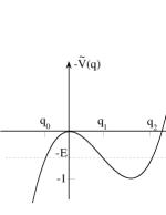
Figure 10: Turning points $q_{1}$ and $q_{2}$ in the potential $-\tilde{V}(q)=-(1/2)\omega_{0}^{2}q^{2}(1-q)$, $\omega_{0}=\sqrt{27/2}$. The “energy” $E$ ($0<E<1$) is determined as a function of inverse temperature $\beta$ by requiring that the motion between the turning points $q_{1}$ and $q_{2}$ is periodic, with period $\beta h$.

Let us consider finite-temperature effects, although the discussion of the last subsection was limited to zero temperature. Then the bounce solution Eq. (56) turns into the periodic solution, i.e., the classical solution in the potential $-\tilde{V}(q)$ [Eq. (54)] with energy $-E$ $(0<E<1)$ Zweger . From Fig. 10 the explicit solution is given by the elliptic function

$$q_{B}(s)=q_{2}-(q_{2}-q_{1}){\text{sn}}^{2}\left(\frac{\omega_{0}}{2}\sqrt{q_{2}-q_{0}}s;m\right)$$ (62)

with $m=\sqrt{(q_{2}-q_{1})/(q_{2}-q_{0})}$, and the period $T$ is given by the complete elliptic integral of the first kind $K(m)$,

$$T=\frac{4}{\omega_{0}\sqrt{q_{2}-q_{0}}}K(m).$$ (63)

The period $T$ is related to the temperature, $T=h\beta$, where $\beta$ is the inverse temperature normalized by $U_{0}$. This solution reduces, of course, to the previous solution Eq. (56) for $E=0$. The corresponding bounce action is evaluated as

$$\tilde{S}_{B}(\beta) = \int_{0}^{h\beta}ds\left[\frac{1}{2}\left(\frac{dq_{B}}{ds}\right)+\tilde{V}(q)\right]$$ (64)

$$= W+h\beta E,$$ (65)

where

$$W = \frac{4}{15}\omega_{0}\sqrt{q_{2}-q_{0}}$$ (66)

$$\times[2(q_{0}^{2}+q_{1}^{2}+q_{2}^{2}-q_{0}q_{1}-q_{0}q_{2}-q_{1}q_{2})E(m)$$

$$+(q_{1}-q_{0})(2q_{0}-q_{1}-q_{2})K(m)]$$

with the complete elliptic integral of the second kind $E(m)$. The decay rate by MQT takes the form

$$\Gamma(\beta)=\frac{A(\beta)}{\tau_{0}}\exp\left({-\frac{\tilde{S}_{B}(\beta)}{h}}\right).$$ (67)

The prefactor $A(\beta)$ was derived in Ref. Yasui as

$$A(\beta)=\sqrt{\frac{\omega_{0}^{3}}{2\pi h}}(q_{2}-q_{0})^{3/4}(q_{2}-q_{1})(1-m^{2})$$

$$\times[a(m)E(m)+b(m)K(m)]^{-1/2}\sinh{\left(\frac{\omega_{0}\beta h}{2}\right)}$$ (68)

with

$$a(m)=2(m^{4}-m^{2}+1),$$ (69)

$$b(m)=(1-m^{2})(m^{2}-1).$$ (70)

The thermal effect increases the MQT rate by a factor of only the order of unity from the MQT rate at zero temperature.

For $E\rightarrow 0$, we have $(1-m^{2})\sinh(\omega_{0}\beta h/2)\rightarrow 8$, $a(m)E(m)+b(m)K(m)\rightarrow 2$, and $q_{0},q_{1}\rightarrow 0$, $q_{2}\rightarrow 1$, so that $A(\beta)\rightarrow 4\sqrt{\omega_{0}^{3}/\pi h}$, which reproduces the zero-temperature decay rate $\Gamma$ of Eq. (57). Let us turn to the limit $E\rightarrow 1$, where the period behaves as

$$\beta h=\frac{2\pi}{\omega_{0}}\left(1+\frac{5}{36}(1-E)+\cdot\cdot\cdot\right).$$ (71)

The leading term gives the crossover temperature $\beta_{c}^{-1}=h\omega_{0}/2\pi$. As the temperature is raised above $\beta_{c}^{-1}$, the system has no bounce solutions, and the decay is caused by thermal activation (the Arrhenius law): $\Gamma_{\beta}\sim\omega_{0}\exp({-\beta\Delta V})$. The crossover temperature is of the order of $0.1$nK for the range of $\delta$ discussed in the last subsection.

Equation (67) and the Arrhenius formula are not available in the narrow region near $\beta_{c}$. In this region the decay rate is given by Affleck

$$\Gamma(\beta)\tau_{0} \simeq \sqrt{\frac{8\omega_{0}^{3}}{15h\pi^{2}}}{\text{sinh}}\left(\frac{\omega_{0}\beta h}{2}\right){\text{erf}}\left[\sqrt{\frac{36}{5\beta_{c}}}(\beta-\beta_{c})\right]$$ (72)

$$\times\exp\left[-\beta+\frac{18\beta_{c}}{5}\left(\frac{\beta-\beta_{c}}{\beta_{c}}\right)^{2}\right],$$

with the error function

$${\text{erf}}(x)=\frac{1}{\sqrt{2\pi}}\int_{-\infty}^{x}dy\exp\left(-\frac{y^{2}}{2}\right).$$ (73)

For small $h\ll 10^{-2}$, this formula matches smoothly onto Eq. (67) for $\beta>\beta_{c}$ and the Arrhenius formula for $\beta<\beta_{c}$ near $\beta_{c}$. However, we cannot apply the formula Eq. (72) to MQT since the value of $h$ in our situation is of the order of $10^{-1}$. We leave the issue of the crossover region for future study.

IV CONCLUSIONS AND DISCUSSION

The metastability and MQT of two-component BECs were studied theoretically. By analyzing two coupled GPEs numerically, we obtained two kinds of metastable state, the symmetry-breaking state (SBS) and the symmetry-preserving states (SPS), which depend on the particle numbers and the interspecies interaction. We introduced the collective coordinate method by improving the usual Gaussian variational approach, and calculated the MQT rate within the WKB approximation. The effective potential $V(Q)$ was determined by analysis of the linear stability and using the saddle-point solution. Then the decay rate is found to obey a scaling law near the critical region. MQT from the SBS to the SPS is expected to be observed in a wide range of the parameter $\delta$. We also predicted MQC between the SBS and the SPS, although the range of $\delta$ is rather narrow.

Our analysis is restricted to the one-dimensional condensate, but it can be applied to a system in a highly anisotropic trapping potential. The extension to the three-dimensional system is troublesome. However, the qualitative nature will be the same as in the one-dimensional case. This analysis can also be applied to the MQT between the domains of a spinor condensate Miesner where the external magnetic field can be used as another variable parameter.

In Sec. II.2 we stated that negative eigenvalues always exist for the SBS, corresponding to the change of particle number. This instability may be caused by inelastic collisions of atoms in a real system. However, if we confine ourselves to the region near the critical particle number, MQT is expected to be the dominant mechanism of decay Ueda . Thus the change of particle number is neglected in the analysis of the MQT.

Finally, we comment on the validity of the quasi-one-dimensional approximation. In this paper, we used the atom-atom interaction Eqs. (3). This would be modified for atoms in a one-dimensional confining potential such as an atom waveguide or a cigar-shaped potential. According to Ref. Olshanii , a two-body potential of the atoms in such a confining potential can be written as

$$U_{\rm 1D}(x)=\delta(x)\frac{2\pi\hbar^{2}a}{m}\frac{1}{\pi b_{\perp}^{2}}\left(1-1.4603\frac{a}{b_{\perp}}\right)^{-1},$$ (74)

where $b_{\perp}=\sqrt{\hbar/m\omega_{\perp}}$. For $b_{\perp}\gg a$, which our parameter $b_{\perp}\simeq 0.29$ $\mu\text{m}$ satisfies, Eq. (74) is smoothly reduced to Eq. (3).

References

- (1) C. J. Myatt, E. A. Burt, R. W. Ghrist, E. A. Cornell, and C. E. Wieman, Phys. Rev. Lett. 78, 586 (1997).
- (2) J. Stenger, S. Inouye, D. M. Stamper-Kurn, H.-J. Miesner, A. P. Chikkatur, and W. Ketterle, Nature (London) 396, 345 (1998).
- (3) H.-J. Miesner, D. M. Stamper-Kurn, J. Stenger, S. Inouye, A. P. Chikkatur, and W. Ketterle, Phys. Rev. Lett. 82, 2228 (1999); D. M. Stamper-Kurn, H.-J. Miesner, A. P. Chikkatur, S. Inouye, J. Stenger, and W. Ketterle, ibid. 83, 661 (1999).
- (4) T. L. Ho and V. B. Shenoy, Phys. Rev. Lett. 77, 3276 (1996).
- (5) B. D. Ersy, C. H. Greene, J. P. Burke, and J. L. Bohn, Phys. Rev. Lett. 78, 3594 (1997).
- (6) H. Pu and N. P. Bigelow, Phys. Rev. Lett. 80, 1130 (1998); 80, 1134 (1998).
- (7) P. Öhberg and S. Stenholm, Phys. Rev. A 57, 1272 (1998).
- (8) E. P. Bashkin and A. V. Vagov, Phys. Rev. B 56, 6207 (1997).
- (9) E. Timmermans, Phys. Rev. Lett. 81, 5718 (1998).
- (10) B. D. Ersy and C. H. Greene, Phys. Rev. A 59, 1457 (1999).
- (11) P. Ao and S. T. Chui, Phys. Rev. A 58, 4836 (1998); 59, 1473 (1999).
- (12) M. Trippenbach, K. Góral, K. Rzaźewski, B. Malomed, and Y. B. Band, J. Phys. B 33, 4017 (2000).
- (13) B. Tanatar and K. Erkan, Phys. Rev. A 62, 053601 (2000).
- (14) D. Gordon and C. M. Savage, Phys. Rev. A 58, 1440 (1998).
- (15) P. Öhberg, Phys. Rev. A 59, 634 (1999).
- (16) C. K. Law, H. Pu, N. P. Bigelow, and J. H. Eberly, Phys. Rev. Lett. 79, 3105 (1997).
- (17) C. C. Bradley, C. A. Sackett, J. J. Tollett, and R. G. Hulet, Phys. Rev. Lett. 75, 1687 (1995).
- (18) H. T. C. Stoof, J. Stat. Phys. 87, 1353 (1997); M. Ueda and A. J. Leggett, Phys. Rev. Lett. 80, 1576 (1998); C. Huepe, S. Métens, G. Dewel, P. Borckmans, and M. E. Brachet, ibid. 82, 1616 (1999); J. A. Freire and D. P. Arovas, Phys. Rev. A 59, 1461 (1999).
- (19) M. Olshanii, Phys. Rev. Lett. 81, 938 (1998).
- (20) D. S. Petrov, M. Holzmann, and G. V. Shlyapnikov, Phys. Rev. Lett. 84, 2551 (2000).
- (21) E. V. Goldstein, M. G. Moore, H. Pu, and P. Meystre, Phys. Rev. Lett. 85, 5030 (2000).
- (22) M. R. Matthews, D. S. Hall, D. S. Jin, J. R. Ensher, C. E. Wieman, E. A. Cornell, F. Dalfovo, C. Minniti, and S. Stringari, Phys. Rev. Lett. 81, 243 (1998).
- (23) S. Inouye, M. R. Andrews, J. Stenger, H.-J. Meisner, D. M. Stamper-Kurn, and W. Ketterle, Nature (London) 392, 151 (1998); Ph. Courteille, R. S. Freeland, D. J. Heinzen, F. A. van Abeelen, and B. J. Verhaar, Phys. Rev. Lett. 81, 69 (1998); S. L. Cornish, N. R. Claussen, J. L. Roberts, E. A. Cornell, and C. E. Wieman, ibid. 85, 1795 (2000).
- (24) H. Kleinert, Path Integrals in Quantum Mechanics, Statistics, and Polymer Physics, (World Scientific, Singapore, 1990).
- (25) In the case of a single condensate, the collective coordinate space is three dimensional, corresponding to the sizes of the condensate along , , and directions. One of the authors (Y.Y.) studied the bounce trajectory by solving the imaginary-time equation of motion analytically and numerically Yasui . It was shown that the trajectory is approximately straight when the number of condensed bosons is slightly below a certain critical number.
- (26) F. R. Klinkhamer and N. S. Manton, Phys. Rev. D 30, 2212 (1984).
- (27) W. Zweger, Z. Phys. B: Condens. Matter 51, 301 (1983).
- (28) Y. Yasui, T. Takaai, and T. Ootsuka, J. Phys. A 34, 2643 (2001).
- (29) I. Affleck, Phys. Rev. Lett. 46, 388 (1981).