Mesoscopic effects in tunneling between parallel quantum wires

Abstract

We consider a phase-coherent system of two parallel quantum wires that are coupled via a tunneling barrier of finite length. The usual perturbative treatment of tunneling fails in this case, even in the diffusive limit, once the length $L$ of the coupling region exceeds a characteristic length scale $L_{t}$ set by tunneling. Exact solution of the scattering problem posed by the extended tunneling barrier allows us to compute tunneling conductances as a function of applied voltage and magnetic field. We take into account charging effects in the quantum wires due to applied voltages and find that these are important for one-dimensional–to–one-dimensional tunneling transport.

I Introduction

Tunneling provides a powerful tool to probe electronic properties of matter.[1] Its sensitivity to momentum-resolved spectral features is determined by geometrical details of the tunnel junction. For example, this sensitivity is completely lost when tunneling occurs via a point contact, whereas it is maximal for an extended, clean tunneling barrier. Since the experimental study of tunneling between two separately contacted, parallel, vertically separated two-dimensional (2D) electron systems became possible,[2] electronic structure and interaction effects in low dimensions have been the subject of careful investigation. In the ideal case, conservation of canonical momentum in the plane of the 2D electron systems leads to sharp tunneling resonances; allowing for exploration of electronic subband energies,[3] mapping of the 2D Fermi surface,[4] and life-time measurements of 2D Fermi-liquid quasiparticles.[5] Modification of one of the 2D layers into a superlattice of one-dimensional (1D) quantum wires has been employed to measure vertical tunneling between 1D and 2D electron systems.[6] Constraints on tunneling imposed by the requirement of simultaneous conservation of energy and momentum can be tuned by the transport voltage and external magnetic fields. In certain situations,[7] this makes it possible to observe features of the momentum-resolved single-electron spectral function directly in tunneling transport.

The method of cleaved-edge overgrowth[8] (CEO) makes it possible to create long and clean quantum wires in GaAs/GaAlAs heterostructures.[9] Using the same technique, systems of two parallel quantum wires with a high and extremely clean tunneling barrier between them have been fabricated in double-layer structures.[10] This opens up new possibilities for studying the peculiar dynamics of electrons in interacting 1D systems[11, 12] using 1D–to–1D tunneling.[13] In particular, both the phase-coherence length and the elastic mean free path $l_{\text{el}}$ for electrons in these quantum wires usually exceed the wire length.[14] This motivates the present work where we analyze mesoscopic effects in 1D–to–1D transport. In related contexts, phase-coherent transport in double-wire systems was discussed in terms of device applications. For example, a system of two parallel, identical quantum wires coupled within a spatial region of length $L<l_{\text{el}}$ via an adjustable tunneling barrier[15] was proposed as a possible realization of a current switch.[16] Wave packets of electrons injected into one of the wires will be coherently transferred to the other one and back with frequency $2|t|/\hbar$. (Here we denoted the tunnel-splitting of energy levels in the coupling region by $2|t|$.) In steady state, this results in a coherent charge oscillation in real space with wave length $L_{t}^{(0)}=\pi\hbar v_{\text{F}}/|t|$. Modulation of $|t|$ controls the signal at the output of the injecting wire. Ideally, it is maximal (minimal) when the ratio of $L$ and $L_{t}^{(0)}$ is (half-)integer. In reality, output characteristics depend sensitively on details of the tunneling barrier.[17] Assuming the feasibility to engineer barrier design, coupled quantum wires were suggested[18] as realizations of quantum logical gates.

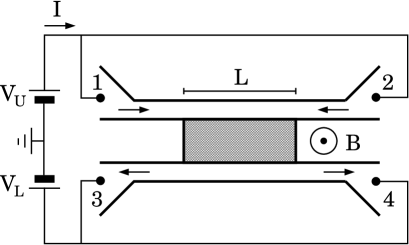
FIG. 1.: Schematic setup for a system of two parallel quantum wires. The magnetic field $B$ allows tuning of kinetic vs. canonical momentum. A voltage $V_{\text{U(L)}}$ is applied uniformly to the upper (lower) wire, i.e., raises the chemical potential of both left-movers and right-movers. The parts of the wires outside the region of space where the barrier is finite are leads to ideal reservoirs. For simplicity, we assume leads of infinite length in our model description.

In this paper, we consider phase-coherent transport in a system of parallel quantum wires coupled via a finite tunneling barrier. See Fig. 1. Charging effects in the wires caused by applied voltages influence tunneling in an important way because they determine the degree to which 1D subbands are shifted or filled. The basic physics of this interplay is discussed in the following section. Our microscopic model for the double-wire system is introduced in the first part of Sec. III. Apart from capacitance effects, interactions are neglected within our approach, which is therefore valid only for voltages and in-plane magnetic fields probing the 1D electron systems beyond the cut-off for Luttinger-liquid behavior.[11] Results from lowest-order perturbation theory are compared with the exact solution using scattering theory. We calculate linear and differential conductances for 1D–to–1D tunneling transport, and discuss their features in Sec. IV.

II Effect of an applied voltage

In the typical tunneling experiment, a voltage drop $V$ across the barrier drives a current. Microscopically, it is often assumed that the voltage shifts quasiparticle bands in the two subsystems by $\pm eV/2$, respectively, as compared to the equilibrium situation where no net current flows. The external circuit is supposed to prevent charging of the subsystems.[19] In general, however, the applied voltage will shift the bands as well as partly fill them. As the I–V curve for 1D–to–1D tunneling depends sensitively on the scenario of band filling vs. band shifting, we discuss this issue here in some detail.

At zero temperature, the free energy (per length) of a 1D system is given by its total energy (per length) $E_{\text{tot}}$ which is a functional of particle density $n$. In a clean quantum wire, $n=n_{0}$ will be constant. Before applying a voltage, the system is assumed to be charge-neutral, i.e., the uniform electronic charge density $en_{0}$ is compensated by positive background and image charges. It is useful to divide $E_{\text{tot}}$ into two parts; $E_{\text{tot}}=E_{\text{int}}+E_{\text{Coul}}$. All Coulombic terms (including the Hartree energy of electrons in the wire) are collected in $E_{\text{Coul}}$, and $E_{\text{int}}$ is the internal energy of the quantum wire comprising kinetic and exchange-correlation contributions. For our purposes, we adopt the simple model with $E_{\text{Coul}}=(e\Delta n)^{2}/2\tilde{C}$ where $\Delta n$ is the deviation from the neutralized charge density $n_{0}$, and $\tilde{C}$ denotes the electrostatic capacitance per unit length of the wire.[20] The applied voltage is assumed to lead to a uniform shift $eV$ with respect to the equilibrium chemical potential $\mu_{0}=\left.\partial E_{\text{tot}}/\partial n\right|_{n_{0}}$ of the wire.[21] The induced change $\Delta n$ in the total density has to be calculated from

$$\mu_{0}+eV=\frac{e^{2}}{\tilde{C}}\,\Delta n+\left.\frac{\partial E_{\text{int}}}{\partial n}\right|_{n=n_{0}+\Delta n}\quad.$$ (1)

In the limit of small voltages ($|eV|\ll\mu_{0}$) where linear-response theory is valid, we can use

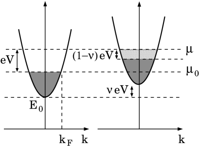
FIG. 2.: A voltage $V$ applied to a quantum wire results, in general, both in a uniform shift of the 1D subband and charging of the wire. Outside the linear-response regime, the parameter $\nu$ depends on voltage. In the double-wire system, a self-consistent treatment of charging effects due to the voltage and tunneling is necessary unless tunneling is weak.

$$\left.\frac{\partial E_{\text{int}}}{\partial n}\right|_{n=n_{0}+\Delta n}-\mu_{0}\approx\frac{\Delta n}{D_{0}}\quad.$$ (2)

Here, $D_{0}$ is the thermodynamic[22] density of states (DOS) defined by $D_{0}=\left.\partial n/\partial\mu\right|_{\mu=\mu_{0}}=\big{(}\partial^{2}E_{\text{int}}/\partial n^{2}\big{)}^{-1}_{n=n_{0}}$. In the linear-response limit, it is then possible to express $\Delta n$ explicitly in terms of the external voltage,[23]

$$\Delta n=eV\,\,\frac{D_{0}}{1+\zeta}\quad,$$ (3)

where the parameter $\zeta$ measures the relative importance of Coulombic and density-of-states effects:

$$\zeta=\frac{e^{2}}{\tilde{C}}\,D_{0}\quad.$$ (4)

We see that, for $\zeta\ll 1$, a voltage will simply fill quasiparticle bands without shifting them (band-filling limit). In particular, this applies in the absence of electron-electron interactions. In the opposite case $\zeta\gg 1$, an applied voltage shifts the bands (band-shifting limit). This situation is analogous to that of a bulk metal or a single-electron transistor.[24] To get an idea of the situation realized in our system of interest, we estimate the capacitance of a quantum wire by $\tilde{C}=2\pi\epsilon/\ln(R/r)$, with $R$ being the distance to surrounding metal gates, and $r$ denoting the characteristic transverse dimension of the wire. Typical values are $\sim 10^{-10}$ F/m. With Fermi energies of quantum wires ranging between $1\dots 10$ meV, we obtain $\zeta\sim 1\dots 10$. Hence, typical quantum wires are in the intermediate regime where both band-filling and band-shifting occurs at the same time. This case is illustrated in Fig. 2. It is important to keep in mind, however, that Eqs. (3) and (4) are only valid when $\Delta n\ll n_{0}$. In experiment, voltages comparable to and larger than $\mu_{0}$ are applied to probe the full single-particle dispersion relation.[10] Then, for a quantitative comparison between theory and experiment, $\Delta n$ has to be found from Eq. (1). For example, a wire whose density was initially large enough for it to be in the band-filling limit crosses over to the band-shifting limit when it is depleted.

At this point, it is useful to make contact with results obtained for Tomonaga-Luttinger (TL) models[25] of interacting 1D electron systems. Unlike their higher-dimensional counterparts, 1D metals cannot be described within the Fermi-liquid paradigm. Instead, their low-energy properties are represented by effective TL models, and the phenomenology of a Luttinger liquid[26] (LL) applies. Instead of Landau parameters, it is the velocities of certain collective and zero-mode excitations that determine all physical quantities of a LL. In particular, the ratio $r_{\text{N}}=v_{\text{N}}/v_{\text{F}}$ of the velocity $v_{\text{N}}$ of the charged zero mode[26] and the bare Fermi velocity enters the expression for the electrostatic capacitance per unit length of a Luttinger liquid: $\tilde{C}_{\text{LL}}=e^{2}D_{0}/(r_{\text{N}}-1)$. Here, $D_{0}=1/\pi\hbar v_{\text{F}}$ is the 1D DOS. Using Eq. (4), we find $\zeta_{\text{LL}}=r_{\text{N}}-1$. The non-interacting case where $r_{\text{N}}=1$ corresponds to the band-filling limit, whereas strong Coulomb interactions ($r_{\text{N}}\to\infty$) recover the band-shifting limit. We would like to remark that $r_{\text{N}}$ constitutes an independent parameter in the low-energy theory of any given real quasi-1D system. It is unrelated, except in certain special cases,[27] to the famous interaction parameter $K_{\rho}$ that enters power-law expressions for electronic correlation functions.[11] From now on, we consider the model where $r_{\text{N}}>1$ but $K_{\rho}=1$. This approximation is valid to describe current experiments where the wires are probably not long enough for the power-law characteristics of a LL to be observable.[28] Even for infinitely long wires, however, our results apply at energies and wave vectors far enough from the Fermi points where the single-particle spectral function recovers Fermi-liquid-like characteristics.[29]

III Model and Formalism

We consider two quantum wires of infinite length, labeled U(pper) and L(ower), that are parallel to the $x$ direction and located, in the $yz$ plane, at $y=0$ and $z=z_{\text{U,L}}$. The potential barrier between them is assumed to be finite and uniform in the region $|x|\leq L/2$ and infinite otherwise. Within the standard notation of second quantization, the Hamiltonian for our system is given by

$$H = \sum_{\alpha=\text{U,L}}H_{\alpha}+H_{\text{tun}}\quad,$$ (6)

$$H_{\alpha} = \int\!\frac{dk}{2\pi}\,\,\epsilon_{\alpha}(k)\,c_{k\alpha}^{\dagger}c_{k\alpha}\quad,$$ (7)

$$H_{\text{tun}} = \int_{-L/2}^{L/2}\!\!dx\left\{t\,\psi^{\dagger}_{\text{U}}(x)\psi_{\text{L}}(x)+{\mathrm{H.c.}}\right\}$$ (8)

$$= \int\!\frac{dk}{2\pi}\int\!\frac{dp}{2\pi}\,\,\left\{t_{k,p}\,c_{k\text{U}}^{\dagger}c_{p\text{L}}+\,\text{H.c.}\right\}\quad.$$ (9)

Here, $\epsilon_{\text{U(L)}}(k)$ is the electronic dispersion relation in the upper (lower) wire. Modulo an unimportant phase factor, the tunneling matrix element is given by[30]

$$t_{k,p}=2|t|\,\frac{\sin\left[(p-k)L/2\right]}{p-k}=|t|\,\sqrt{2\pi L\,\delta_{L}(p-k)}.$$ (10)

The second equality in Eq. (10) constitutes the definition of $\delta_{L}(p-k)$ which is a finite-size realization of Dirac’s $\delta$-function. Tunneling occurs mainly between states with momenta satisfying $|p-k|<2\pi/L$. Perfect momentum conservation holds only in the limit $L\rightarrow\infty$.

We consider the case where a single (the lowest) 1D subband in each wire is occupied and assume a parabolic subband dispersion. The effect of a magnetic field $\vec{B}=B\,\hat{y}$ applied perpendicularly to the plane of the two wires can be included by a shift of kinetic with respect to canonical momentum.[31] Then, dispersion relations read ($\alpha=\text{U,L}$)

$$\epsilon_{\alpha}(k)=\frac{\hbar^{2}}{2m}\left(k-\frac{eB}{\hbar}\,z_{\alpha}\right)^{2}+E_{0\alpha}+\nu_{\alpha}\,eV_{\alpha}\quad.$$ (11)

Here, $m$ is the effective electron mass in the semiconductor host medium, and $E_{0\alpha}$ denotes the energy at the bottom of the respective wire’s lowest 1D subband. The term $\nu_{\text{U(L)}}eV_{\text{U(L)}}$ takes into account the shifting of the band in the upper (lower) wire due to an applied voltage. See Fig. 2. For simplicity, we neglect effects due to the mutual capacitance of the two wires, which can be included straightforwardly. In general, the values of $\nu_{\alpha}$ will depend on voltage. Furthermore, except in the limit of weak tunneling where $|t|\ll|eV_{\alpha}|$, they have to be determined from a self-consistent treatment of charging effects resulting from tunneling and electrostatics. While this is, in principle, straightforward to implement, we choose to focus here on the weak-tunneling limit which is more relevant for current experiment.[10] In the linear-response regime, we have $\nu_{\alpha}=\zeta_{\alpha}/(1+\zeta_{\alpha})$ with $\zeta_{\alpha}$ defined for each wire in analogy to Eq. (4).

Absolute values of energy and the $z$ coordinate are irrelevant; results depend only on the difference of subband energies, $\Delta E_{0}=E_{\text{0L}}-E_{\text{0U}}$, and the wire separation, $d=z_{\text{U}}-z_{\text{L}}$. For simplicity, we choose $E_{\text{0U}}=0$ and $z_{\text{U}}=0$ in the following. Also, to avoid cluttering the notation, we have suppressed spin quantum numbers. In typical CEO structures, the effect of Zeeman splitting is negligible for the range of magnetic fields to be considered below.[32] Hence, electron spin leads only to factors of 2 which we include in our final formulae for tunneling current and conductances.

A Perturbation theory: Lowest order in tunneling

A standard procedure[19, 33] for calculating the tunneling current is to perform perturbation theory in $H_{\text{tun}}$. To leading order, the current flowing from the upper to the lower wire is

$$I = \frac{2e}{\hbar}\int\!\frac{dk}{2\pi}\int\!\frac{dp}{2\pi}\,\,|t_{k,p}|^{2}\int_{-\infty}^{\infty}\!\frac{d\epsilon}{2\pi}\,\,A_{\text{U}}(\epsilon,k)A_{\text{L}}(\epsilon,p)$$ (13)

$$\hskip 113.81102pt\times\left[f_{\text{U}}(\epsilon)-f_{\text{L}}(\epsilon)\right]\quad,$$

with Fermi functions $f_{\alpha}(\epsilon)=1/[1+\exp\{(\epsilon-\mu_{0}-eV_{\alpha})/k_{\text{B}}T\}]$. The single-particle spectral functions for the wires are given, within the model specified above, by $A_{\alpha}(\epsilon,k)=2\pi\delta[\epsilon-\epsilon_{\alpha}(k)]$. In the linear-response limit ($|eV_{\alpha}|\ll\mu_{0}$), we find the tunneling conductance

$$G=\frac{2e^{2}}{\hbar^{3}}\frac{|t|^{2}L}{v_{\text{FU}}v_{\text{FL}}}\sum_{\gamma,\gamma^{\prime}=\pm 1}\delta_{L}\left(\frac{\pi}{2}[\gamma n_{\text{U}}-\gamma^{\prime}n_{\text{L}}]-p_{\text{B}}\right)\,.$$ (14)

Here, $v_{\text{F}\alpha}$ and $n_{\text{F}\alpha}$ denote the Fermi velocity and electron density of the respective wire at the equilibrium chemical potential $\mu_{0}$. The peak-shape function $\delta_{L}$ has been defined in Eq. (10), and the relative shift of the 1D Fermi seas due to the applied magnetic field is $p_{\text{B}}=-eB\,d/\hbar$.

In analogy to 2D–to–2D tunneling,[4] resonances appear in the tunneling conductance $G$ as function of magnetic field whenever parts of the shifted Fermi surfaces of the two wires overlap. As the 1D Fermi surface consists of just two points, the shape of these resonances is that of a smeared delta function of width $2\pi/L$. The peak value of the tunneling conductance can be written as

$$G_{\text{pk}}=n^{*}\,\frac{2e^{2}}{h}\,\,\left(\frac{\pi L}{L_{t}}\right)^{2}\quad,$$ (15)

where $L_{t}=\pi\hbar\sqrt{v_{\text{FU}}v_{\text{FL}}}/|t|$ is an effective length scale introduced by tunneling, and $n^{*}=1$ or $2$ depending on the number of overlapping Fermi points at peak condition.

In the dirty limit[34] where the length $L$ of the tunneling barrier is larger than the mean free path $l_{\text{el}}$, Eq. (14) is still valid but the peak width is now given by $2\pi/l_{\text{el}}$. Also, the factor $(\pi L/L_{t})^{2}$ in Eq. (15) has to be replaced by $2\pi^{2}L\,l_{\text{el}}/L^{2}_{t}$. In both the ballistic and diffusive cases, taking the limit of $L\to\infty$ is unphysical: the conductance through the barrier cannot exceed $2e^{2}/h$ per channel. Hence, the actual small parameter enabling perturbative treatment of tunneling is $L/L_{t}$. Smallness of $L/L_{t}$ means that the time between tunneling events has to be larger than the time it takes electrons to traverse the region where the potential barrier between the wires is finite. Only then it will be possible to neglect higher-order effects due to electrons tunneling coherently back and forth between the wires. Using the exact solution developed in the next subsection, we will find indeed that the perturbative result displayed in Eq. (14) is valid only as long as $L\ll L_{t}$.

B Exact solution using scattering theory

As the model defined in Eqs. (III) describes two systems of noninteracting fermionic quasiparticles that are coupled via tunneling in a finite region of space, we can use scattering theory for calculating transport.[35] To make this explicit, we rewrite the Hamiltonian of our system in first-quantized notation and real-space representation. It is a $2\times 2$ matrix [because wave functions are two-component spinors $(\psi_{\text{U}},\psi_{\text{L}})^{\mathrm{T}}$]:

$$H=\left(\begin{array}[]{lr}\epsilon_{\text{U}}(-i\partial_{x})&t(x)\\ t(x)&\epsilon_{\text{L}}(-i\partial_{x})\end{array}\right)\quad.$$ (16)

The tunneling matrix element is piecewise constant: $t(x)=|t|$ for $|x|\leq L/2$ and $t(x)=0$ otherwise. Hence, regions with $|x|>L/2$ where the wires are independent act as leads where scattering states can be defined. We attach labels 1 through 4 to these leads as shown in Fig. 1. The region $|x|\leq L/2$ where tunneling occurs acts as an effective scatterer. The current flowing through the tunnel barrier is then given by

$$I=\frac{2e}{h}\sum_{m=1,2\atop n=3,4}\int d\epsilon\,\left|T_{m,n}(\epsilon)\right|^{2}\left[f_{\text{U}}(\epsilon)-f_{\text{L}}(\epsilon)\right]\quad,$$ (17)

where $T_{m,n}(\epsilon)$ denotes the transmission coefficient for electrons with energy $\epsilon$ that originate in lead $m$ and are scattered into lead $n$. We calculate the transmission coefficients by matching scattering states in the leads to the appropriate eigenstates of the Hamiltonian (16) in the region $|x|\leq L/2$. As this is a straightforward exercise, and results for the most general case are lengthy, we omit explicit formulae here. Due to the difference of Fermi functions in Eq. (17), only transmission coefficients $T_{m,n}(\epsilon)$ at energies within the voltage window, i.e., with $\epsilon-\mu_{0}\in[eV_{\text{L}},eV_{\text{U}}]$, contribute. In the limit of small applied voltage, Eq. (17) yields the linear conductance

FIG. 3.: Linear conductance for two identical wires, calculated exactly (solid curve) and with perturbation theory (dashed curve). Inset: Oscillation of conductance in zero magnetic field (solid) and with $p_{\text{B}}=0.001\,k_{\text{F}}^{(0)}$ (dotted) where $k_{\text{F}}^{(0)}$ is the Fermi wave vector for zero magnetic field.

$$G=\frac{2e^{2}}{h}\sum_{m=1,2\atop n=3,4}\left|T_{m,n}(\mu_{0})\right|^{2}\quad.$$ (18)

As expected, $G$ obtained from Eq. (18) deviates from the perturbative result [Eq. (14)] for long enough barrier length $L$, see Fig 3. The oscillatory dependence of $G$ on $L$ can be tuned by the applied magnetic field, as seen in the inset of Fig. 3. When the effective tunnel splitting in the coupling region is much smaller than the Fermi energy of the quantum wires, the following approximate formula for the linear conductance can be derived (see the Appendix for details):

$$G\approx\frac{2e^{2}}{h}\sum_{\gamma,\gamma^{\prime}=\pm 1}\frac{\sin^{2}\left(\pi\sqrt{\left(L/L_{t}\right)^{2}+\left(L/L_{\gamma\gamma^{\prime}}\right)^{2}}\right)}{1+(L_{t}/L_{\gamma\gamma^{\prime}})^{2}}\quad.$$ (19)

Here, new length scales $L_{\gamma\gamma^{\prime}}$ appear that measure the mismatch of canonical Fermi momentum for pairs of Fermi points from the upper (right-mover $\gamma=+1$, left-mover $\gamma=-1$) and lower ($\gamma^{\prime}$ analogous) wires:

$$L_{\gamma\gamma^{\prime}}=\frac{2\pi}{\frac{\pi}{2}\left[\gamma n_{\text{U}}-\gamma^{\prime}n_{\text{L}}\right]-p_{\text{B}}}\quad.$$ (20)

Exact calculation of $G$ in the appropriate limit confirms the validity of Eq. (19); see Fig. 4.

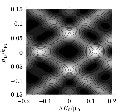
FIG. 4.: Contour plot of the linear conductance $G$ vs. $\Delta E_{\mathrm{0}}$ and $p_{\mathrm{B}}$ for $L=L_{t}^{(0)}=100/k_{\text{F}}^{(0)}$. (Here, $L_{t}^{(0)}$ and $k_{\text{F}}^{(0)}$ are the tunneling length and Fermi wave vector when $\Delta E_{0}=0$ and $B=0$. Due to our gauge choice, $k_{\text{FU}}=\pi n_{\text{U}}/2$ is unaffected by the external magnetic field.) The oscillatory structure is well-described by Eq. (19). For our choice of parameters, $G=0$ at in-resonance condition. Note that tuning the magnetic field near off-resonance maxima (e.g., for $\Delta E_{0}=0$ and $p_{\text{B}}=0.07\,k_{\text{FU}}$) has a strong effect on $G$.

IV Results and Discussion

Different regimes in the behavior of the linear 1D–to–1D tunneling conductance are distinguished by the interplay of the relevant length scales encountered above. These are the length $L$ of the tunnel barrier, $L_{t}$ which is a measure of the strength of tunneling, and lengths $L_{\gamma\gamma^{\prime}}$ which are defined for any pairing of a Fermi point from the upper wire with one from the lower wire. For the following discussion, we consider only the largest $L_{\gamma\gamma^{\prime}}$ of all possible. Comparing $L_{t}$ with the other lengths, a weak-tunneling regime ($L_{t}>\max\{L_{\gamma\gamma^{\prime}},L\}$) can be distinguished from a strong-tunneling regime ($L_{t}<\max\{L_{\gamma\gamma^{\prime}},L\}$). Furthermore, we call the system in resonance when the Fermi points of a corresponding $L_{\gamma\gamma^{\prime}}$ are close to each other on the scale of $2\pi/L$, i.e., when $L<L_{\gamma\gamma^{\prime}}$. Conversely, the off-resonance limit is reached for $L>L_{\gamma\gamma^{\prime}}$.

In the strong-tunneling regime, the linear conductance oscillates as a function of $L$ with wave length $L_{t}$ and maximum amplitude $2e^{2}/h$ ($4e^{2}/h$ for identical wires). Previously, when the feasibility of using the double-wire system as a directional coupler was discussed, the in-resonance limit was considered only.[16] Control of directional-coupler operation is then possible only by varying $L_{t}$, i.e., essentially only by adjusting the barrier height. Here we find that, in the off-resonance limit, the device is tunable, in addition to varying $t$, by an applied magnetic field or, equivalently, by adjusting the density mismatch in the two wires. This is seen already in the inset of Fig. 3 and, more clearly, in Fig. 4. It is, therefore, possible to adjust the effective length scale for coherent electron transfer between the wires by applying a magnetic field. When $L$ is equal to several times $L_{t}$, the difference between the effective transfer length in a magnetic field and $L_{t}$ leads to an accumulated phase shift over many oscillations that can reach $\pi/2$ without concomitant loss in amplitude. In particular for CEO structures, operating the system in off-resonance mode provides a convenient alternative to any (hardly feasible) adjustment of the high tunnel barrier.

The weak-tunneling limit is well-suited for spectroscopic application of 1D–to–1D tunneling. Sharp peaks are exhibited by both the linear and differential conductances for in-resonance conditions. Measured on the scale of resonance peaks, the off-resonance conductance is orders of magnitude smaller. We have calculated the differential conductance as a function of magnetic field and voltage whose resonance condition corresponds to a Fermi point of one wire coinciding with a point on the dispersion curve of the other wire. The exact location of these coincidences in the $V$–$B$ plane depends sensitively on charging effects in the quantum wires. In the following, we focus on the limit of weakly coupled wires where the self-consistent charge profile is not importantly affected by tunneling. Furthermore, we consider the situation with symmetric bias $V_{\text{U}}=-V_{\text{L}}=V/2$.

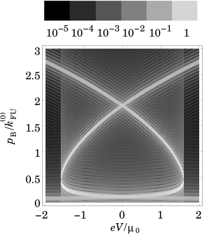
FIG. 5.: Differential conductance for 1D–to–1D tunneling in the ideal band-filling case ($\tilde{C}=\infty$), shown as a logarithmic gray-scale plot in arbitrary units. Parameters used are $\Delta E_{0}=0.2\mu_{0}$ and $k_{\text{FU}}^{(0)}L=100$. $k_{\text{FU}}^{(0)}$ is the Fermi wave vector of the upper wire at zero voltage. The finite width of bright resonance features as well as the appearance of darker maxima is due to the finite length $L$ of the tunnel barrier. Note the symmetry with respect to voltage reversal which is a key feature of the band-filling case.

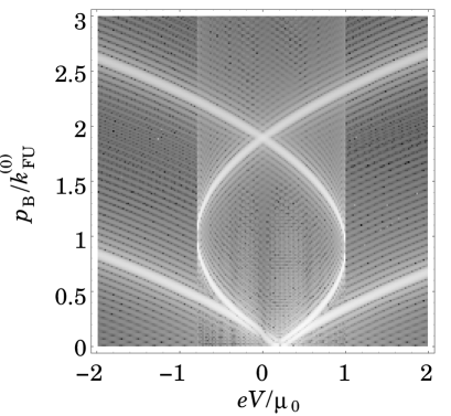
FIG. 6.: Differential conductance for 1D–to–1D tunneling in the ideal band-shifting case ($\tilde{C}=0$). We show a logarithmic gray-scale plot of its absolute value. Parameters and gray-scale units are the same as in Fig. 5. A characteristic feature of the band-shifting case is that the edges of the leaf-shaped structure in the voltage direction are exactly at the Fermi energies of the two wires. The differential conductance is negative on the low-magnetic-field resonance lines.

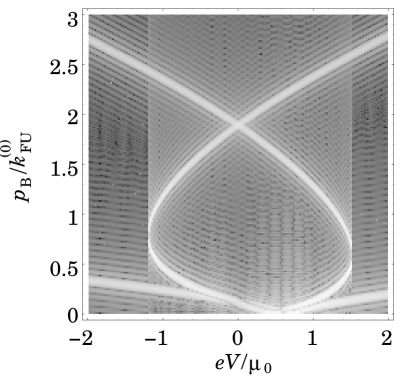
FIG. 7.: Differential conductance for 1D–to–1D tunneling in an intermediate situation with finite $\tilde{C}$. Shown is its absolute value in a logarithmic gray-scale plot. See Fig. 5 for a legend. In addition to the parameters used in Fig. 5, we have $\tilde{C}_{\text{U}}=\tilde{C}_{\text{L}}=8\varepsilon\varepsilon_{0}/(k_{\text{FU}}^{(0)}a_{\text{B}})$ where $a_{\text{B}}$ is the Bohr radius in the semiconductor host material.

Figures 5 and 6, respectively, show logarithmic gray-scale plots of the absolute value of the differential tunneling conductance for the ideal band-filling ($\tilde{C}=\infty$) and band-shifting ($\tilde{C}=0$) cases.[36] Bright lines are formed by points in the $V$–$B$ plane where the above-mentioned resonance condition is fulfilled. Due to the finite length of the tunnel barrier, more maxima appear with peak values being orders of magnitude smaller than at the resonance peaks. In the band-shifting case, resonance lines are direct images of parts of the wires’ electronic dispersion curves. In particular, the extension of the leaf-shaped structure in the positive and negative voltage direction provides a direct measure of the respective wire’s Fermi energy. This is not the case for the band-filling limit, which is characterized by a resonance line running close to the voltage axis when $E_{0}\ll\mu_{0}$. Its leaf structure is symmetric under voltage reversal, with extension in (positive or negative) voltage direction given by $2(\mu_{0}-|\Delta E_{0}|)$. In real systems, the capacitance $\tilde{C}$ is finite, and an intermediate picture will be obtained for the differential tunneling conductance. An example is shown in Fig. 7, where $\tilde{C}$ has a value such that $\zeta_{\text{U}}=0.5$ at zero voltage. Depletion of one of the wires for increasing voltage leads to a cross-over to the band-shifting situation. As a result, the ideal band-shifting limit is not easily distinguished from the intermediate case. Quantitative comparison of the measured resonance structure in the differential conductance with results expected from an independent measurement of Fermi energies, electron densities etc. will have to include the effect of the finite $\tilde{C}$. Conversely, for known Fermi-sea parameters, the value of $\tilde{C}$ can be extracted by fitting the measured resonance pattern of the differential conductance for 1D–to–1D tunneling.

V Conclusions

Motivated by recent experiment, we have investigated linear and differential conductances for 1D–to–1D transport. Our results show that effects due to phase coherence and charging of the wires are important for realistic double-wire structures. Regimes of weak and strong tunneling, as well as in and out of resonance, are distinguished and their key features discussed. We point out new possibilities for device application of 1D–to–1D tunneling and its use for electron-dispersion spectroscopy.

Calculation of transmission coefficients

Equations (17) and (18) express tunneling current and linear conductance in terms of transmission coefficients $T_{m,n}(\epsilon)$. These transmission coefficients can be obtained exactly by matching eigenstates of Hamiltonian $H$ [given in Eq. (16)] with eigenvalue $\epsilon$ in the coupling region ($|x|\leq L/2$) to appropriate eigenstates in the leads. For example, to calculate $T_{1,n}$, we use the ansatz

$$\left.\Psi_{\epsilon}(x)\right|_{x<-\frac{L}{2}} = \left(\begin{array}[]{c}1\\ 0\end{array}\right)e^{ik_{\text{U}}^{(+)}x}$$ (24)

$$+ \left(\begin{array}[]{c}t_{11}\\ 0\end{array}\right)e^{ik_{\text{U}}^{(-)}x}+\left(\begin{array}[]{c}0\\ t_{13}\end{array}\right)e^{ik_{\text{L}}^{(-)}x}\,,$$ (29)

$$\left.\Psi_{\epsilon}(x)\right|_{x>\frac{L}{2}} = \left(\begin{array}[]{c}t_{12}\\ 0\end{array}\right)e^{ik_{\text{U}}^{(+)}x}+\left(\begin{array}[]{c}0\\ t_{14}\end{array}\right)e^{ik_{\text{L}}^{(+)}x}\,,$$ (34)

$$\left.\Psi_{\epsilon}(x)\right|_{|x|<\frac{L}{2}} = \sum_{\alpha=\text{a,b}}\left\{d_{+}^{(\alpha)}\left(\begin{array}[]{c}u_{+}^{(\alpha)}\\ v_{+}^{(\alpha)}\end{array}\right)e^{ik_{+}^{(\alpha)}x}\right.$$ (40)

$$\hskip 28.45274pt+\left.d_{-}^{(\alpha)}\left(\begin{array}[]{c}u_{-}^{(\alpha)}\\ v_{-}^{(\alpha)}\end{array}\right)e^{ik_{-}^{(\alpha)}x}\right\}\,.$$

Here, wave vectors $k_{\text{U(L)}}^{(\pm)}$ are solutions of $\epsilon\equiv\epsilon_{\text{U(L)}}(k_{\text{U(L)}}^{(\pm)})$ with positive ($+$) and negative ($-$) group velocity $v_{\text{U(L)}}=\partial_{\hbar k}\epsilon_{\text{U(L)}}(k)$, respectively. With the energy dispersion in the coupling region given by $\epsilon_{\pm}(k)=\frac{1}{2}\left[\epsilon_{\text{U}}(k)+\epsilon_{\text{L}}(k)\right]\pm|t|\sqrt{1+r^{2}}$, we have $\epsilon\equiv\epsilon_{\pm}\big{(}k_{\pm}^{(\text{a,b})}\big{)}$. The function $r=[\epsilon_{\text{U}}(k)-\epsilon_{\text{L}}(k)]/2|t|$ measures the mismatch in the dispersions of the two wires and determines the amplitudes $u_{\pm}=\sqrt{(1\pm r/\sqrt{1+r^{2}})/2}$, $v_{\pm}=\pm\sqrt{(1\mp r/\sqrt{1+r^{2}})/2}$. Requiring continuity of the wave function and current conservation at the locations $x=\pm L/2$ yields a system of linear equations from which the coefficients $t_{mn}$ and $d_{\pm}^{(\alpha)}$ are found. Transmission coefficients entering Eqs. (17) and (18) are then given by $T_{m,n}(\epsilon)=t_{mn}\sqrt{|v_{\text{L}}/v_{\text{U}}|}$.

The linear conductance is given in terms of transmission coefficients[35] at the equilibrium chemical potential $\mu_{0}$, as expressed in Eq. (18). To derive Eq. (19), we consider, e.g., $T_{1,4}$. When the tunnel splitting $2|t|$ and Fermi-energy mismatch of the two wires is much smaller than their Fermi energies, only amplitudes for right-moving partial waves in ansatz (Calculation of transmission coefficients) are significantly different from zero. Neglecting left-moving partial waves and the small density mismatch, the matching procedure yields $t_{14}=i\sin(k_{t}L)/\sqrt{1+r^{2}}$ with $k_{t}=t\sqrt{1+r^{2}}/\hbar v_{\text{F}}$. In the regime considered, we have $r\approx L_{t}/L_{11}$ with $L_{11}$ defined in Eq. (20). Similar calculations for other transmission coefficients finally yield Eq. (19).

REFERENCES

- [1] E. L. Wolf, Principles of Electron Tunneling Spectroscopy, Vol. 71 of International Series of Monographs in Physics (Oxford University Press, New York, 1985); F. Capasso, Physics of Quantum Electron Devices, Vol. 28 of Springer Series in Electronics and Photonics (Springer, Berlin, 1990).
- [2] J. Smoliner, E. Gornik, and G. Weimann, Appl. Phys. Lett. 52, 2136 (1988); J. P. Eisenstein, L. N. Pfeiffer, and K. W. West, Appl. Phys. Lett. 58, 1497 (1991).
- [3] J. Smoliner, W. Demmerle, G. Berthold, E. Gornik, G. Weimann, and W. Schlapp, Phys. Rev. Lett. 63, 2116 (1989); W. Demmerle, J. Smoliner, G. Berthold, E. Gornik, G. Weimann, and W. Schlapp, Phys. Rev. B 44, 3090 (1991).
- [4] J. P. Eisenstein, T. J. Gramila, L. N. Pfeiffer, and K. W. West, Phys. Rev. B 44, 6511 (1991); L. Zheng and A. H. MacDonald, Phys. Rev. B 47, 10619 (1993).
- [5] S. Q. Murphy, J. P. Eisenstein, L. N. Pfeiffer, and K. W. West, Phys. Rev. B 52, 14825 (1995); T. Jungwirth and A. H. MacDonald, Phys. Rev. B 53, 7403 (1996).
- [6] J. Smoliner, W. Demmerle, F. Hirtler, E. Gornik, G. Weimann, M. Hauser, and W. Schlapp, Phys. Rev. B 43, 7358 (1991); W. Demmerle, J. Smoliner, E. Gornik, G. Böhm, and G. Weimann, Phys. Rev. B 47, 13574 (1993); B. Kardynał, C. H. W. Barnes, E. H. Linfield, D. A. Ritchie, K. M. Brown, G. A. C. Jones, and M. Pepper, Phys. Rev. Lett. 76, 3802 (1996); B. Kardynał C. H. W. Barnes, E. H. Linfield, D. A. Ritchie, J. T. Nicholls, K. M. Brown, G. A. C. Jones, and M. Pepper, Phys. Rev. B 55, R1966 (1997).
- [7] U. Zülicke and A. H. MacDonald, Phys. Rev. B 54, R8349 (1996); A. Altland, C. H. W. Barnes, F. W. J. Hekking, and A. J. Schofield, Phys. Rev. Lett. 83, 1203 (1999).
- [8] L. Pfeiffer, K. W. West, H. L. Stormer, J. P. Eisenstein, K. W. Baldwin, D. Gershoni, and J. Spector, Appl. Phys. Lett. 56, 1697 (1990); M. Grayson, Ç. Kurdak, D. C. Tsui, S. Parihar, S. Lyon, and M. Shayegan, Solid-State Electron. 40, 233 (1996).
- [9] A. Yacoby, H. L. Stormer, N. S. Wingreen, L. N. Pfeiffer, K. W. Baldwin, and K. W. West, Phys. Rev. Lett. 77, 4612 (1996).
- [10] O. M. Auslaender and A. Yacoby, in preparation.
- [11] J. Voit, Rep. Prog. Phys. 57, 977 (1994).
- [12] D. Carpentier, C. Peça, and L. Balents, cond-mat/0103193; U. Zülicke and M. Governale, cond-mat/0105066.
- [13] Parallel quantum wires have been fabricated before using a split-gate technique. See K. J. Thomas, J. T. Nicholls, M. Y. Simmons, W. R. Tribe, A. G. Davies, and M. Pepper, Phys. Rev. B 59, 12252 (1999). In this experiment, 1D–to–1D tunneling transport was not measured directly. Instead, the two-terminal conductance of the two wires in parallel was used for spectroscopy of the tunnel-split 1D subbands.
- [14] R. de Picciotto, H. Stormer, A. Yacoby, L. N. Pfeiffer, K. W. Baldwin, and K. W. West, Phys. Rev. Lett. 85, 1730 (2000).
- [15] C. C. Eugster, J. A. del Alamo, M. J. Rooks, and M. R. Melloch, Appl. Phys. Lett. 64, 3157 (1994).
- [16] J. A. del Alamo and C. C. Eugster, Appl. Phys. Lett. 56, 78 (1990).
- [17] M. Macucci, A. Galick, and U. Ravaioli, Phys. Rev. B 52, 5210 (1995); M. Governale, M. Macucci, and B. Pellegrini, Phys. Rev. B 62, 4557 (2000).
- [18] A. Bertoni, P. Bordone, R. Brunetti, C. Jacoboni, and S. Reggiani, Phys. Rev. Lett. 84, 5912 (2000).
- [19] D. Rogovin and D. J. Scalapino, Ann. Phys. (NY) 86, 1 (1974).
- [20] Our modeling of electrostatics using the single parameter is a first approximation to the real situation where, e.g., coupling to reservoirs leads to a non-uniform distribution of electron density as well as charge transfer between reservoirs and the wire. See, e.g., V. A. Sablikov, S. V. Polyakov, and M. Büttiker, Phys. Rev. B 61, 13763 (2000).
- [21] Here, in contrast to the situation considered in Refs. [37, 38, 39, 40, 41], the external voltage does not drive a net current flow within a single quantum wire.
- [22] In contrast to the familiar single-particle density of levels, the thermodynamic DOS contains exchange-correlation contributions.
- [23] M. Büttiker, H. Thomas, and A. Prêtre, Phys. Lett. A 180, 364 (1993); M. Büttiker, J. Phys.: Condens. Matter 5, 9361 (1993); M. Büttiker and T. Christen, in: Mesoscopic Electron Transport, edited by L. L. Sohn, L. P. Kouwenhoven, and G. Schön (Kluwer Academic, Dordrecht, 1997), pp. 259-289.
- [24] See, e.g., M. A. Kastner, Rev. Mod. Phys. 64, 849 (1992); Single Charge Tunneling, edited by H. Grabert and M. H. Devoret (Plenum Press, New York, 1992). Within the language used in the literature studying single-electron effects, the parameter corresponds to the ratio of charging energy to the single-particle level spacing.
- [25] S. Tomonaga, Prog. Theor. Phys. 5, 544 (1950); J. M. Luttinger, J. Math. Phys. 4, 1154 (1963).
- [26] F. D. M. Haldane, J. Phys. C 14, 2585 (1981).
- [27] Y. M. Blanter, F. W. J. Hekking, and M. Büttiker, Phys. Rev. Lett. 81, 1925 (1998); R. Egger and H. Grabert, Phys. Rev. B 55, 9929 (1997), ibid. 58, 13275(E) (1998).
- [28] The characteristic length scale above which LL effects will be important can be roughly estimated by . Here, is a cut-off wave number that can be much smaller than . We expect quantum wires in CEO structures to be at the borderline of this criterion; see O. M. Auslaender, A. Yacoby, R. de Picciotto, K. W. Baldwin, L. N. Pfeiffer, and K. W. West, Phys. Rev. Lett. 84, 1764 (2000).
- [29] K. Schönhammer and V. Meden, Phys. Rev. B 48, 11390 (1993).
- [30] M. Governale, M. Grifoni, and G. Schön, Phys. Rev. B 62, 15996 (2000).
- [31] This neglects the finite size of the wires in direction.
- [32] The range of magnetic fields that need to be applied to map out the interesting features in the linear, or differential, tunneling conductance implies the condition for safe neglect of Zeeman splitting. Here, is the Landé factor, the electron mass in vacuum, and the (in general, voltage-dependent) electron density in the wire. Typically, this condition will be violated only in the band-filling limit around the point where one of the wires is empty.
- [33] G. D. Mahan, Many-Particle Physics (Plenum Press, New York, 1990).
- [34] Elastic scattering by impurities is taken into account by introducing a finite life-time broadening for the single-electron spectral functions .
- [35] R. Landauer, IBM J. Res. Dev. 1, 223 (1957); M. Büttiker, IBM J. Res. Dev. 32, 306 (1988); S. Datta, Electron Transport in Mesoscopic Systems (Cambridge University Press, Cambridge, UK, 1995).
- [36] In Figs. 5–7, we give in units of which is independent of magnetic field due to our gauge choice.
- [37] D. L. Maslov and M. Stone, Phys. Rev. B 52, R5539 (1995).
- [38] V. Ponomarenko, Phys. Rev. B 52, R8666 (1995).
- [39] I. Safi and H. J. Schulz, Phys. Rev. B 52, R17040 (1995).
- [40] R. Egger and H. Grabert, Phys. Rev. Lett. 77, 538 (1996), ibid. 80, 2255(E) (1998).
- [41] R. Egger and H. Grabert, Phys. Rev. B 58, 10761 (1998).