Power law correlations in the Southern Oscillation Index fluctuations characterizing El Ni$\tilde{n}$o

Abstract

The southern oscillation index ($SOI$) is a characteristic of the El Ni$\tilde{n}$o phenomenon. $SOI$ monthly averaged data is analyzed for the time interval 1866-2000. The tail of the cumulative distribution of the fluctuations of $SOI$ signal is studied in order to characterize the amplitude scaling of the fluctuations and the occurrence of extreme events. Large fluctuations are more likely to occur than the Gaussian distribution would predict. The time scaling of fluctuations is studied by applying the energy spectrum and the Detrended Fluctuation Analysis ($DFA$) statistical method. Self-affine properties are found to be pertinent to the $SOI$ signal and therefore suggest power law correlations of fluctuations of the signal. Antipersistent type of correlations exist for a time interval ranging from about 4 months to about 6 years. This leads to favor specific physical models for El Ni$\tilde{n}$o description.

El Ni$\tilde{n}$o is one of the most fascinating phenomena in meteorology. Its consequences are thought to be wide ranged and sometimes catastrophic. There is no fundamental explanation, even though much work has been performed on the subject.[1] One basic function characterizing el Ni$\tilde{n}$o is the so-called southern oscillation index ($SOI$). The cyclic warming and cooling of the eastern and central regions in the Pacific Ocean are coupled to distinctive sea level pressures. The normalized difference between the pressure measured at Darwin and the pressure measured at Tahiti are used to generate the so-called $SOI$ number. When the number is negative there is an El-Ni$\tilde{n}$o (or ocean warming), but when the number is positive, there is a La-Ni$\tilde{n}$a effect (or ocean cooling). Indeed the central and eastern Pacific regions of the ocean are normally colder than its equatorial location would suggest, mainly due to the influence of northeasternly trade winds, a cold ocean current flowing up the coast of Chile, and to the up-welling of cold deep water off the coast of Peru. At times, the influence of these cold water sources wane, causing the surface of the eastern and central Pacific to warm up under the tropical sun.

There is already a large number of $SOI$ analyses.[2, 3, 4, 5] Here we analyze the southern oscillation index monthly averaged data for the time interval 1866-2000, i.e. 1612 data points.[6, 7] Even though this is a limited number of data points, it is possible to study the amplitude and time scaling of the fluctuations of the $SOI$ data by calculating the power spectrum and applying the Detrended Fluctuation Analysis statistical method ($DFA$)[8] with acceptable error bars. The latter technique has already demonstrated its usefulness in turbulence,[9] in biology for sorting out coding and non-coding sequence behavior in DNA,[10] in financial analysis for characterizing e.g. currency exchange rates,[11, 12] and in other self-organizing critical systems[13] for time series with similar lengths.

We do not aim at forecasting[14] here. Forecasting models already exist for El-Ni$\tilde{n}$o events, through the sea-surface temperature canonical correlation analysis ($CCA$) model,[15, 16] the coupled ocean/atmosphere model,[17] and the linear inverse model[18] to mention a few of them.

Note also, an excellent, detailed intercomparison of three different forecasting models that have predicted moderate warming of the equatorial Pacific sea surface temperatures (SSTs) to begin in late summer to early fall of 1986.[15] One of the models includes sea level pressure data, a quantity that is subject to our study. This is a statistical model, that is designed to predict sea surface temperature from prior variations of the sea level pressure. Authors draw a conclusion that the key to the success of the model is recognizing the large-scale, low-frequency changes in the tropical ocean-atmospheric system. They based their conclusion on the estimate of the relative importance of the prior data, included in the model, for the subsequent predictive skill of the model.

The present work stresses the implications of correlations in the amplitude and time scaling of the fluctuations of $SOI$. In so doing, a selected choice between proposed models can be envisaged.

I Data

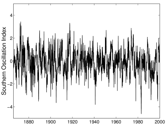
Data for years 1866-2000 were obtained from Ref.[6] and Ref.[7]. They are plotted as function of time (in month units) in Fig. 1. The data consists of $1612$ data points and represent monthly averaged normalized difference between the pressure measured at Darwin and the sea level pressure measured at Tahiti. For the years before 1866 daily measurements of the sea level pressure at both stations have been reported to exist and monthly values of the southern oscillation index have been calculated [19] back to 1841. However, there are gaps of a couple of years in the record whence not suitable for our analysis.

II Distribution of fluctuations

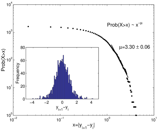
First, we calculate the fluctuations $y_{i+1}-y_{i}$ of the $SOI$ signal $y(t)$, group them into bins with size equal to the difference between the maximum and the minimum of the fluctuations and divide by one hundred, i.e. $~{}0.082$. Then we count the number of entries inside each bin. The result is the histogram shown in the inset of Fig. 2. The distribution of fluctuations of the $SOI$ signal is symmetrical and not Gaussian.

Next we focus on the tails as they characterize how likely the extreme events are to occur. We calculate the empirical probability to observe fluctuations with an amplitude larger than some value, $Prob(X>x)$, where $x=|y_{i+1}-y_{i}|$. The result is plotted in Fig. 2 (dots). The tail of this distribution is consistent with a power law $Prob(X>x)\sim x^{-\mu}$, showing the reduction of the probability for increasing intensity of the fluctuations. A linear least-squares fit yields an estimate $\mu=3.30\pm 0.06$ when the amplitudes of fluctuations are between 1.5 and 2.8. It is difficult to have good estimate for larger amplitudes of the fluctuations (between 3 and 4) due to insufficient statistics. Note, that the $\mu$-value is well outside the range for stable Lévy distributions, $0<\mu<2$, and in particular outside the Gaussian distribution ($\mu=2$). Therefore, large fluctuations are more likely to occur than the Gaussian distribution would predict.

The cumulative probability distribution provides an estimate for the intensity structure, e.g. the amplitude scaling of the fluctuations of the $SOI$ signal. The asymptotic power law behavior of the intensity distribution of the fluctuations appears to be a particularly suitable description of the occurrence of extreme events. In the next section we will focus on the time scaling and correlations of the fluctuations of the $SOI$ signal.

III $SOI$ temporal correlations

We apply two methods to study the temporal correlations of fluctuations in the $SOI$ signal, spectral and the detrended fluctuation analysis methods.

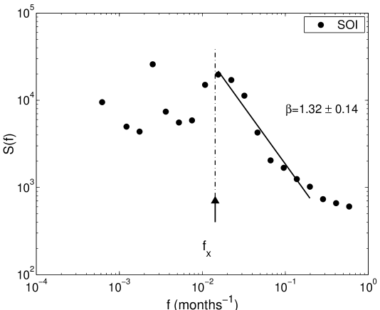
The spectral analysis involves calculating of the power spectrum as a Fourier transform of the data. To quantify the correlations of the fluctuations in a signal the scaling properties of its power spectrum are tested. Assuming a power-law behavior of the energy spectrum $S(f)\sim f^{-\beta}$ the self-affine properties of the signal are characterized by the $\beta$-value.

In Fig. 3 results from the spectral analysis of the $SOI$ data are plotted. For the frequency range from 1/5 to 1/64 months^-1 the spectrum is consistent with a power-law behavior with a spectral exponent $\beta=1.32\pm 0.14$. However such Fourier transform analyses fall short of precisely showing crossover regimes. To better estimate the crossover and to test the correlations using a different approach, we analyze the $SOI$ signal applying the $DFA$ technique.[8]

The detrended fluctuation function $F(\tau)$ is calculated following

$${{F^{2}(\tau)}}={1\over\tau}{\sum_{t=k\tau+1}^{(k+1)\tau}{\left[y(t)-z(t)\right]}^{2}},{\hskip 28.45274pt}k=0,1,2,\cdots,({N\over\tau}-1),$$ (1)

where $z(t)=at+b$ is a linear least-square fit to the data points in a box containing $\tau$ points.

The behavior of the averaged though other forms for $z(t)$ can be used [20] $F^{2}(\tau)$ over the $N/\tau$ intervals with length $\tau$ is expected to be a power law

$$\langle F^{2}(\tau)\rangle\sim\tau^{2\alpha}.$$ (2)

An exponent $\alpha\not=1/2$ in a certain range of $\tau$ values implies the existence of long-range correlations in that time interval as, for example, in fractional Brownian motion [21, 22, 23]. A value of $\alpha<0.5$ indicates antipersistence and $\alpha>0.5$ implies persistence of correlations. The classical random walk (Brownian motion) is such that $\alpha=1/2$.

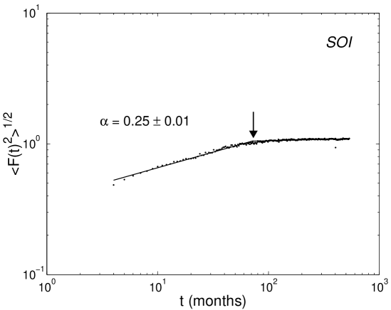
In Fig. 4, a log-log plot of the function $\sqrt{\langle F^{2}(\tau)\rangle}$ is shown for the $SOI$ data in Fig. 1. This function is close to a power law with an exponent $\alpha_{1}=0.25\pm 0.01$ holding for the interval time ranging from about 4 to 70 months. In contrast to the Fourier spectrum analysis the crossover of the fluctuations function $<F^{2}(\tau)>$ is well defined at 70 months. For time scales longer than 70 months, i.e. about 6 years, a crossover to noise-like $\alpha_{2}=0.05\pm 0.009$ is observed. This suggests antipersistence of the correlations in the fluctuations of the sea level pressure for time lags less than 6 years. Antipersistence of the fluctuations implies that a positive fluctuation in the past is more likely to be followed by a negative fluctuation in the future.

Note that $\alpha=Hu$, $Hu$ being the so called Hurst exponent. The Hurst exponent of a signal was first defined in the “rescaled range (R/S) analysis” (of Hurst [24, 25]) to estimate the correlations in the Nile floodings and droughts. The relationship

$$\beta=2Hu+1$$ (3)

has been theoretically proven by Flandrin for fractional Brownian walks.[26] The $\alpha_{1}$ value for the $SOI$ signal is consistent within the error bars with the spectral exponent satisfying the above equation.

IV Conclusions

We have studied the amplitude, time scaling and correlations of the fluctuations of the Southern Oscillation Index ($SOI$). The tail of the cumulative distribution of the $SOI$ fluctuations is found to scale with an exponent $\mu=3.3$ for amplitudes of the fluctuations between 1.5 and 2.8, describing the occurrence of extreme events. The energy spectrum of the $SOI$ is consistent with power law with exponent $\beta=1.32$ for the frequency range between 1/5 and about 1/64 months. Since $1<\beta<3$ the $SOI$ signal is a self-affine fractal.[22] To estimate more precisely the crossover regime and the type of correlations we have applied the $DFA$ method. Using the $DFA$ method we find an antipersistent type of correlations for time lags less than 70 months. The $\alpha$-exponent that characterizes the scaling is consistent within the error bars with the spectrum scaling. This leads to favor specific physical models for El Ni$\tilde{n}$o description, as that in Ref.[15].

Our analysis shows that long-range correlations exist between the fluctuations of the $SOI$, e.g. sea level pressure. This supports one conclusion in Ref.[[15]] pertinent to our analysis, i.e. the large-scale low-frequency variations of the global SLP field are responsible for the predictive skill of the sea level pressure forced statistical model. The present work indicates a hint why it might be so: because of the correlations between the fluctuations.

Acknowledgments

We thank T.P. Ackerman, H.N. Shirer and E.E. Clothiaux for stimulating discussions and comments. This investigation was partially supported by grant number Battelle 327421-A-N4. The comments of C. Nicolis are greatly appreciated.

FIG. 1.: The monthly values of the Southern Oscillation Index for the period 1866 to April 2000 representing the standardized pressure difference between Tahiti and Darwin stations ($1612$ data points).

FIG. 2.: The empirical probability to observe fluctuations with amplitude larger than some value $x=|y_{i+1}-y_{i}|$. An asymptotic power law scaling is found for fluctuation amplitudes between 1.5 and 2.8. Histogram of the fluctuations of the $SOI$ signal is shown in the inset.

FIG. 3.: The energy spectrum of the $SOI$ data (from Fig. 1). A spectral exponent $\beta=1.32\pm 0.14$ characterizes the correlations of fluctuations in the frequency range from about 1/5 to about 1/64 months^-1.

FIG. 4.: The DFA-function $<F^{2}(\tau)>^{1/2}$ in log-log plot for the $SOI$ data from Fig. 1. Two scaling regimes are observed, $\alpha_{1}=0.25\pm 0.01$ and noise-like $\alpha_{2}=0.05\pm 0.009$ with a crossover at 70 months.

REFERENCES

- [1] There are several websites where information and data are available; see e.g. http://www.pmel.noaa.gov/toga-tao/el-nino/forecasts.html http://www.cpc.ncep.noaa.gov/ http://ingrid.ldgo.columbia.edu/SOURCES/.Indices/ensomonitor.html
- [2] C. Nicolis, Tellus, 42A, 401-412 (1990).
- [3] C. Frankignoul and K. Hasselmann, Tellus, 29 289-305 (1977).
- [4] K. Fraedrich, Monthly Weather Review, 116 1001 (1988).
- [5] T.N. Palmer Rep. Prog. Phys., 63 71 (2000).
- [6] Thanks to James Mather from University of Wisconsin who referred us to:
- [7] http://www.cpc.ncep.noaa.gov/data/indices/
- [8] C.-K. Peng, S.V. Buldyrev, S. Havlin, M. Simons, H.E. Stanley, and A.L. Goldberger, Phys. Rev. E 49, 1685 (1994).
- [9] S. Ghashghaie, W. Breymann, J. Peinke, P. Talkner and Y. Dodge, Nature 381, 767 (1996).
- [10] H.E. Stanley, S.V. Buldyrev, A.L. Goldberger, S. Havlin, C.-K. Peng, and M. Simons, Physica A 200, 4 (1996).
- [11] N. Vandewalle and M. Ausloos, Physica A 246, 454 (1997).
- [12] K. Ivanova and M. Ausloos, Physica A 270, 526 (1999).
- [13] P. Bak, K. Chen and M. Creutz, Nature 342, 780 (1989).
- [14]
- [15] T. Barnett, N. Graham, M. Cane, S. Zebiak, S. Dolan, J. O’Brien, and D. Legler, Science, 241 192 (1988)
- [16] A.G. Barnston and C.F. Ropelewski, Journal of Climate, 5, 1316 (1992).
- [17] M. Ji, D.W. Behringer, A. Leetmaa, Monthly Weather Review 126, 1022 (1998).
- [18] C. Penland and T. Magorian, Journal of Climate, 6, 1067 (1993).
- [19] G.P. Konnen, P.D. Jones, M.H. Kaltofen, R.J. Allan, Journal of Climate, 11, 2325 (1998).
- [20] N. Vandewalle and M. Ausloos, Int. J. Comput. Anticipat. Syst. 1, 342 (1998).
- [21] B.J. West and W. Deering, Phys. Rep. 246, 1 (1994).
- [22] J. West, The Lure of Modern Science: Fractal Thinking, (World Scient., Singapore, 1995)
- [23] P.S. Addison, Fractals and Chaos, (Institute of Physics, Bristol, 1997)
- [24] H.E. Hurst, Trans. Amer. Soc. Civil Eng. 116, 770 (1951).
- [25] J. Feder, Fractals, (Plenum, New York, 1988)
- [26] P. Flandrin, IEEE Trans. Information Theory, 35, 197 (1989).