Critical dynamics and universality of the random-bond Potts  
ferromagnet with tri-distributed quenched disorders  

Abstract

Critical behavior in short-time dynamics is investigated by a Monte Carlo study for the random-bond Potts ferromagnet with a trinary distribution of quenched disorders on two-dimensional triangular lattices. The universal dynamic scaling is verified and applied to estimate the critical exponents $\theta$, $z$ and $\beta/\nu$ for several realizations of the quenched disorder distribution. Our critical scaling analysis strongly indicates that the bond randomness influences the critical universality.

I Introduction

The study of the critical properties of physical systems with bond randomness on phase transitions is a quite active field of current interest in equilibrium statistical physics Cardy96 ; Cardy99 . One of the central importance here is to answer the question whether the critical exponents (of a homogeneous pure magnet) change on the addition of quenched impurities and, if so, how do they change? Replying to this question, it was first stated already two decades ago that if the specific heat critical exponent $\alpha$ of a pure system is positive, then a quenched disorder is a relevant perturbation at the second-order critical point and it causes changes in critical exponents. This statement is known as the Harris criterion Harris . Furthermore, following the earlier work of Imry and Wortis Imry79 , who argued that quenched disorder could smooth first-order phase transitions and thus produce the second-order phase transitions, the introduction of randomness to pure systems undergoing a first-order transition has been comprehensively considered Hui89 ; Aizen89 . The theory was initially numerical checked with the Monte Carlo (MC) method by Chen, Ferrenberg and Landau (CFL) Chen92 , who studied the 8-state random-bond Potts model with a bimodal self-dual distribution. On the other hand the experimental evidence has been found that, for the order-disorder phase transitions of absorbed atomic layers on two-dimensions, the critical exponents are changed from the original universality class of the 4-state Potts model on the addition of disorders Schwen94 ; Voges98 . However, no modification is found when the pure system belongs to the Ising universality class Mohan98 . Recently such disordered systems are extensively studied by examining how a phase transition is modified by quenched disorder coupling to the local energy density Folk00 , where use of intensive MC simulations is often helpful Wise95 ; Kardar95 ; Yasar98 ; Chate98a ; Olson99 .

The two-dimensional (2D) $q$-state random-bond Potts ferromagnet (RBPF) is an interesting framework in the MC research to study the influence of impurity on pure systems. For $q>2$ such randomness acts as a relevant perturbation, and for $q>4$ it even changes the nature of the transition from first to second order. In Table 1 we list the magnetic scaling index $\beta/\nu$ of the 2D 8-state RBPF obtained by different groups. Here a disorder amplitude $r$, defined by the ratio of the strong to weak coupling (distributed according to the bimodal distribution) in the range $r=$2-20 appears to be adapted to a numerical analysis and gives a good estimate of the disordered fixed point exponents Cardy99 ; Picco98 . A recent work of Olson and Young Olson99 used a specially continuous self-dual probability distribution of the disoreded bonds

$$P_{X}(x)=\frac{2\sqrt{q}}{\pi(1-x)^{2}+qx^{2}}~{}~{}~{}~{}~{}$$ (1)

for the Boltzmann factor $x\equiv e^{-K}$, and performed a MC study of multiscaling properties of the correlation functions for several values of $q$. Their results are very interesting to examine the universality class of the RBPF. Cardy and Jacobsen Cardy97 studied the RBPF based on the connectivity transfer matrix (TM) formalism Jaco98 , and their estimates of the critical exponents lead to a continuous variation of $\beta/\nu$ with $q$, which is in sharp disagreement with the MC results by CFL(see Table 1).

Authors	$r$	$\beta/\nu$	Technique
CFLChen92	2,10	0.118(2)	MC
Chatelain and BercheChate98a	10	0.152(3)	MC
Olson and YoungOlson99	$P_{X}(x)$	0.156(3)	MC
PiccoPicco98	10	0.153(1)	MC
Cardy and JacobsenCardy97	2	0.142(4)	TM
Chatelain and BercheChate99	10	0.1505(3)	TM
Ying and HaradaYing00	10	0.151(3)	STD

Table 1: Magnetic exponent $\beta/\nu$ estimated by different groups for the 2D 8-state RBPF.

In this paper, we present a MC study by short-time dynamics (STD) to verify the dynamic scaling features of the RBPF and estimate the critical exponents for a trinary random-bond Potts model on a 2D triangular lattice. It is well known that this model on the 2D triangular lattice belongs to the same universality as the one on the 2D square lattice in equilibrium. However, a difference exists that the transition temperature is changed because the systems on triangular lattices lost the original (square-square) self-duality relation. Instead, a honeycomb-triangular duality (or star-triangular duality) is satisfied Baxter . Therefore the multi-disorder amplitudes $r_{i}$ can be introduced to study the dynamic universality of the RBPF on such lattices by the STD approach Janss89 ; Zheng98 . In particular we will investigate the dynamic behavior of critical scaling affected by introducing quenched randomness, and study the dependence of critical exponents on the randomness strength in order to clarify the crossover behavior (pure $\longleftrightarrow$ random fixed point $\longleftrightarrow$ percolation-like limit) Picco98 .

II The model

The Hamiltonian of the $q$-state Potts model on a 2D triangular lattice with quenched random interactions can be written as

$$-\beta H=\sum_{<i,j>}K_{ij}\delta_{\sigma_{i}\sigma_{j}}=\sum_{\{L_{0}\}}K_{0}\delta_{\sigma_{i}\sigma_{j}}+\sum_{\{L_{1}\}}K_{1}\delta_{\sigma_{i}\sigma_{j}}+\sum_{\{L_{2}\}}K_{2}\delta_{\sigma_{i}\sigma_{j}},~{}$$ (2)

where the spin $\sigma_{i}$, defined on lattice site $i$, takes the values 1, $\cdots~{}q$, $\beta=1/k_{B}T$ is the inverse temperature, $\delta$ the Kronecker delta function and the sum is over all the nearest-neighbor (NN) interactions (bonds) $<i,j>$ on the lattice with a size $N=L^{2}$. There are $3N$ NN bonds (six for each and shared by two spins) and they can be grouped into three classes $\{L_{0},L_{1},L_{2}\}$ corresponding to the interactions on them. The dimensionless couplings $K_{ij}$ can be selected from three positive (ferromagnetic) values $K_{0}$, $K_{1}=r_{1}K_{0}$ and $K_{2}=r_{2}K_{0}$ according to a probability distribution,

$$P(K)=(1-p_{1}-p_{2})\delta(K-K_{0})+p_{1}\delta(K-K_{1})+p_{2}\delta(K-K_{2}).~{}~{}~{}~{}~{}~{}~{}~{}~{}~{}~{}~{}$$ (3)

When $p_{1}=p_{2}=1/3$ it is a trinary random-bond system. By denoting $F_{0}=(e^{K_{c}}-1)$, $F_{1}=(e^{K^{\prime}_{c}}-1)$ and $F_{3}=(e^{K^{\prime\prime}_{c}}-1)$, where $K_{c}$, $K^{\prime}_{c}=r_{1}K_{c}$ and $K^{\prime\prime}_{c}=r_{2}K_{c}$ are the critical values of $K_{0}$, $K_{1}$ and $K_{2}$ respectively, the critical point can be determined by a self-dual relation Baxter ; Kim74 ,

$$F_{0}F_{1}F_{2}+F_{0}F_{1}+F_{0}F_{2}+F_{1}F_{2}=q~{}~{}~{}~{}$$ (4)

for the trinary system with the given state parameter $q$.

The strong to weak coupling ratio $r_{i}=K_{i}/K_{0}$ is called disorder amplitude. The values $r_{1}=0$ or $r_{2}=0$ correspond to the diluted case Mar99 , and $r_{1}=r_{2}=1$ to the pure case where the phase transitions are first-order for $q>4$. With the presence of quenched random-bonds, however, the second-order phase transitions are induced for any $q$-state of the Potts model and the critical points can be calculated according to Eq.(4). In our simulations we chose $q=8$ which is known to have a strong first-order phase transition in the pure cases, in hope that we would find second-order phase transitions induced by the quenched random disorders to demonstrate the influence of quenched impurities on the first-order phase transitions. The strength of disorder is realized by the disorder amplitudes $\{r_{1},r_{2}\}$ as chosen in Table 2. There are three types of such disordered systems for the trinary distribution: (I) one-third bonds chosen randomly are strongly coupled with {$r_{1}$=1, $r_{2}>1$}, (II) two-third bonds strongly coupled with different amplitudes $r_{2}>r_{1}>1$ and (III) two-third bonds with the same amplitude $r_{1}$=$r_{2}>1$. Actually the systems III, 2/3 bonds being strongly coupled with {$r_{1}$=$r_{2}>1$}, are related to those I, 1/3 bonds being strongly coupled, because the former can be transferred to the latter by taking 1/3 bonds to be weakly coupled with {$r_{1}$=1, $r^{\prime}_{2}=1/r_{2}<1$}. The study will be concentrated on the important question whether there exists an Ising-like universality class for systems with multi-quenched randomness Kardar95 ; Chate99 .

I:	II:	III
{$r_{1},r_{2}$}  $T_{c}$	{$r_{1},r_{2}$}  $T_{c}$	{$r_{1},r_{2}$}  $T_{c}$
{1, 5}  .39903934…	{2, 5}  .33624310…	{ 5, 5}  .19047260…
{1, 8}  .29663628…	{5, 8}  .19047260…	{ 8, 8}  .15574523…
{1,10} .25548102…	{8,10} .13987343…	{10,10} .12638846…
{1,12} .22533080…	{2,12} .19784059…	{12,12} .11306096…

Table 2: The critical temperature as a function of disorder amplitudes $\{r_{1}$, $r_{2}\}$ for the trinary RBMF. (I) 1/3 bonds are strongly coupled with $r_{2}>1$, (II) 2/3 bonds are strongly coupled with different amplitudes $r_{2}>r_{1}>1$ and (III) with the same amplitude $r_{1}$=$r_{2}>1$.

III Short-time dynamics

For a long time, it was believed that universality and scaling relations can be found only in equilibrium or in the long-time regime. In Ref.Janss89 , however it was discovered that for an $O(N)$ vector magnetic system in the states with a very high temperature $T\gg T_{c}$, when it is suddenly quenched to the critical temperature $T_{c}$ and evolves according to a dynamics of model A, a universal dynamic scaling behavior emerges already within the short-time regime,

$$M^{(k)}(t,\tau,L,m_{0})=b^{-k\beta/\nu}M^{(k)}(b^{-z}t,b^{1/\nu}\tau,b^{-1}L,b^{x_{0}}m_{0}),$$ (5)

where $M^{(k)}$ is the $k$th moment of magnetization, $t,\tau=(T-T_{c})/T_{c},L$ and $b$ are time, reduced temperature, linear size of the lattice and scaling factor respectively. $\beta$ and $\nu$ are the well known static critical exponents. The quantity $x_{0}$, a new independent exponent, is the scaling dimension of the initial magnetization $m_{0}$. This dynamic scaling form is generalized from finite size scaling in equilibrium.

Up to present, the short-time dynamic MC simulations have been successfully performed to estimate the critical temperatures $T_{c}$ and the critical exponents $\theta$, $\beta$, $\nu$ and the dynamic exponent $z$ for the various models with second order phase transitions Zheng98 . This approach has also been extensively applied for systems with disorders, as the FFXY and spin glass, to estimate both dynamic and static critical exponents Luo98 ; Luo99 , and for systems on the 2D triangular lattices to study the dynamic scaling universality Ying01 . The method is also efficient to study the deterministic dynamics Zheng99 .

We carry out simulations in an analogous strategy described in Ref.Ying00 where the magnetic observables to be measured for the RBPF have been well defined. In this work, however, an additional step is introduced to verify that the second-order phase transitions really are induced when quenched randomness is added. Then we will be particularly concerned to demonstrate the evidence for the dynamic universality of the trinary RBPF. Therefore our MC simulations are mainly performed for the time evolution of the magnetization $M(t)$ from the disordered initial states with small magnetizations $m_{0}\gtrsim 0$, and the completely ordered state with $m_{0}=1$. In the former, the magnetization $M(t)$ undergoes an initial increase at the critical point $K_{c}$ for $t>t_{mic}$,

$$M(t)\sim m_{0}t^{\theta},~{}~{}~{}~{}~{}~{}~{}\theta=(x_{0}-\beta/\nu)/z.~{}~{}~{}~{}$$ (6)

For the latter, with $m_{0}=1$, $M(t)$ shows a power-law decay behavior Ito93

$$M(t)\sim t^{-c_{1}},~{}~{}~{}~{}~{}c_{1}=\beta/\nu z,~{}~{}~{}~{}~{}~{}~{}~{}~{}$$ (7)

at the critical point. Furthermore the Binder cumulant $U(t,L)=M^{(2)}(t,L)/M^{2}(t,L)$ shows, for $m_{0}=1$ at criticality, a similar power-law behavior on a large enough lattice,

$$U(t,L)\sim t^{c_{u}},~{}~{}~{}c_{u}=d/z.~{}~{}~{}~{}~{}$$ (8)

Here the magnetization $M(t)$ is defined by

$$M(t) = \frac{1}{N}\left[\left<(\frac{qM_{o}(t)-N}{q-1})\right>\right],~{}~{}~{}~{}~{}$$ (9)

$M_{o}=\mbox{max}(M_{1},M_{2},\cdots,M_{q})$ with $M_{i}$ being the number of spins in the $i$th state. $N=L^{2}$ is the total number of spins on the lattice. $<\cdots>$ denotes thermal averages over the initial states and/or random number sequences, and $[\cdots]$ the disorder averages over quenched randomness distributions. The time unit $t$ is defined as a MC sweep over all spins on the lattice.

The time-dependent susceptibility (the second moment of the magnetization) is defined as usual

$$M^{(2)}(t) = \frac{1}{N}\left[\left(<M^{2}(t)>-<M(t)>^{2}\right)\right].~{}~{}~{}$$ (10)

It has played an important role in equilibrium to determine the critical exponents $\gamma/\nu$ and $\beta/\nu$ Chen92 .

IV Results

In our simulations, up to 60,000 MC processes are taken for MC averages (300 samples chosen as disorder averages in a given distribution and 100-200 initial configurations as thermal averages for each disorder configuration realization). Statistical errors are simply estimated by performing three groups of averages with different random number sequences as well as independent initial configurations. To minimize the number of bond configurations needed for the disorder averaging, we confine our study to the bond distributions in which there are the same number of disordered (stronger) NN bonds for each of the three groups $\{L_{0},L_{1},L_{2}\}$. This procedure is reliable and should reduce the variation between different disorder configurations with no loss of generality. Periodic boundary conditions are applied to the $N=L^{2}$ lattice. We use $L$ up to 128 and adopt the heat-bath algorithm.

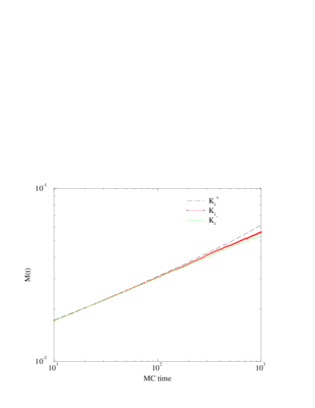
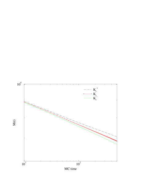
Figure 1: $M(t)$ versus MC time plotted on a log-log scale for {$r_{1}$=1,$r_{2}$=8} from the initial states $m_{0}\sim 0.01$, performed at and near the critical point $K_{c}$ and $K_{c}^{\pm}=(1\pm 0.012)K_{c}$.

Figure 2: The same as Fig.1 but from the ordered states $m_{0}=1$.        

The data for the evolution of $M(t)$ from $m_{0}\gtrsim 0$ and $m_{0}=1$ exhibit that the power-law behavior is satisfied at the same point $K_{c}$ for both the disordered and ordered initial states. This fact gives an evidence that a second-order phase transition is induced at $K_{c}$ instead of a first-order one: In Ref.Schu00 it was argued that there are two quasi-critical points if a first-order transition happens, $K^{random}_{c}$ for evolutions from random initial states and $K^{order}_{c}$ from ordered initial states, and $K^{random}_{c}<K_{c}<K^{order}_{c}$ is satisfied. We plot in Fig.1 and Fig.2 the curves $M(t)$ for disorder amplitudes {$r_{1}$=1, $r_{2}=8$} on a $64^{2}$ lattice. They exhibit obviously a power-law relaxation at the same critical point for both the $m_{0}\gtrsim 0$ and $m_{o}=1$ states. On the other hand the curves deviate from the power-law behavior for a small but nonzero $\tau$ described by $M(t,\tau)=m_{0}t^{\theta}M(t^{1/\nu z}\tau)$ or $M(t,\tau)=t^{-c_{1}}F(t^{1/\nu z}\tau)$ with respect to the disordered or ordered initial states respectively. This modification has been initially used to determine the critical temperatures Schu95 ; Jas99 . The same features, as plotted in Figs. 1 and 2, exist for all other realizations of the randomness listed in Table 2.

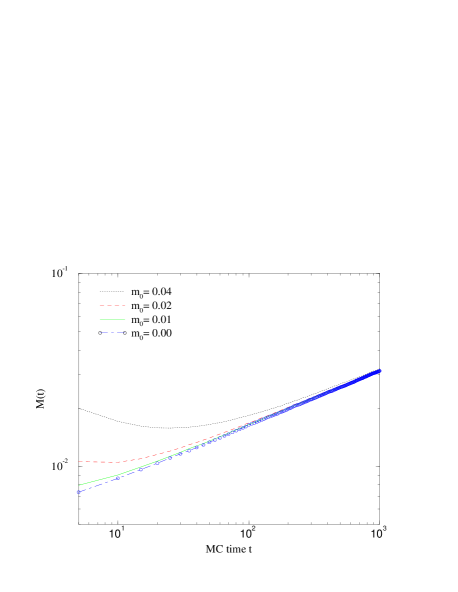
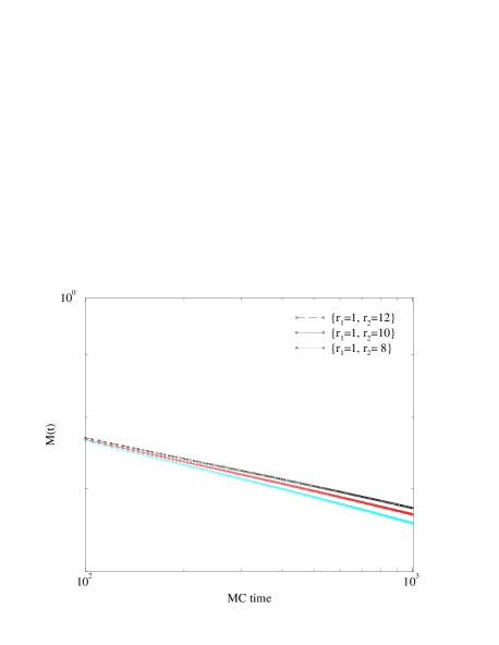
Figure 3: $M(t)$ versus MC time plotted on a log-log scale for {$r_{1}$=5,$r_{2}$=8} from random initial states with magnetizations $m_{0}$=0.04,0.02,0.01 and with $m_{0}\sim 0$ on a $128^{2}$ lattice.

Figure 4: $M(t)$ versus MC time plotted on a log-log scale for {$r_{1}$=1,$r_{2}$=8}, {$r_{1}$=1,$r_{2}$=10} and {$r_{1}$=1,$r_{2}$=12} from the initial states $m_{0}=1$ on a $128^{2}$ lattice.

Then we perform simulations systematically at the exact critical points $K_{c}(r_{i})$ as a function of {$r_{1},r_{2}$} for magnetization evolutions starting with $m_{0}\gtrsim 0$ and $m_{0}=1$. The disordered initial states are prepared from random states with small magnetizations $m_{0}$ = 0.04 – 0.01. The curves $M(t)$ for the disordered configurations with $r_{1}=5$, $r_{2}=8$ on a $128^{2}$ lattice are displayed in Fig.3 with a double-logarithmic scale. They exhibit the power-law behavior of Eq.(6) for $t>t_{mic}$, which depends on $m_{0}$. Thus the exponent $\theta$ can be estimated with the standard least square fitting algorithm, from the slopes of the curves for $t>t_{mic}$, and by an extrapolation to the $m_{0}\rightarrow 0$ limit. The values are included in Table 3. Next we start from $m_{0}=1$ to observe the power-law decay of Eq.(7) at the critical points $K_{c}(r_{i})$. Some curves $M(t)$ are plotted in Fig.4, which appear to have also a nice power-law behavior, and the slopes are then used to estimate the index $c_{1}=\beta/\nu z$ (for results see Table 3).

Now we turn to the dynamic scaling behavior of the time-dependent Binder cumulant from $m_{0}=1$ to estimate the scaling index $c_{u}=d/z$. Unlike the relaxation from the disordered state, the fluctuations involved in the ordered initial states (e.g., $\sigma_{i}$ = 1, $i=1,N$) are much smaller. Therefore, the measurements of the critical exponents based on Eq.(7) and Eq.(8) are better in quality than those from disordered states on Eq.(6). So we take about 100 MC sweeps for random number sequences to be the thermal averages for the completely ordered initial state. In Figs.5 the curves $U(t)$ on a $128^{2}$ lattice are presented and they exhibit a power-law behavior at the critical points as a function of disorder amplitudes {$r_{1}$, $r_{2}$}. Finally, based on the results of $c_{u}=d/z$ and $c_{1}=\beta/\nu z$, the critical exponents $z$ and $\beta/\nu$ can be calculated consistently and their results are summarized in Table 3.

	{$r_{1},r_{2}$}	$\theta$	$c_{1}$	$c_{u}$	$z$	$\beta/\nu$
I:	{ 1, 5}	.238(3)	.0780(8)	.789(6)	2.53(4)	.202(5)
	{ 1, 8}	.206(2)	.0654(7)	.611(6)	3.28(5)	.212(5)
	{ 1,10}	.187(2)	.0597(7)	.599(6)	3.34(5)	.200(5)
	{ 1,12}	.180(2)	.0559(7)	.554(6)	3.61(5)	.202(5)
II:	{ 2, 5}	.268(3)	.0864(9)	.889(6)	2.25(4)	.194(5)
	{ 5, 8}	.283(3)	.0849(9)	.893(7)	2.24(4)	.190(4)
	{ 8,10}	.290(3)	.0830(9)	.897(7)	2.23(4)	.185(4)
III:	{ 5, 5}	.305(4)	.0784(8)	.959(7)	2.09(3)	.164(4)
	{ 8, 8}	.296(3)	.0811(9)	.907(8)	2.21(4)	.179(4)
	{10,10}	.293(3)	.0815(9)	.898(8)	2.23(4)	.182(4)

Table 3: The values of indices ($\theta$,$c_{1}$,$c_{u}$), and results of exponents ($z$, $\beta/\nu$) with respect to the disorder amplitudes $\{r_{1},r_{2}\}$.

V Summary and Conclusion

We have, for the first time, introduced the trinary distribution for the 2D RBPF with multi-disorder amplitudes to study its critical behavior by the STD method. In the MC simulation the dynamic scaling behavior is verified and the power-law behavior is used to estimate both the dynamic and static exponents as a function of the disorder amplitudes $\{r_{1},r_{2}\}$. It is found that the values of exponents $\theta$ and $\beta/\nu$ vary continuously with the disorder amplitudes, and they violate the Ising-like universality. Furthermore the values of dynamic exponent $z$ are larger than those for systems without disorders and they increase with the strength of disorder amplitudes {$r_{1},r_{2}$} for the systems I: $r_{1}=1$, $r_{2}>1$ and III: $r_{1}$=$r_{2}>1$ in Table 3.

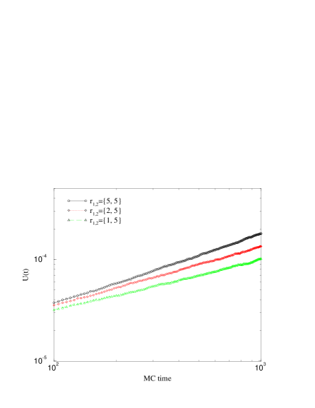
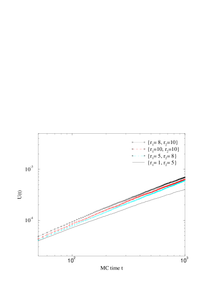
Figure 5: $U(t)$ versus MC time on a log-log scale as a function of the disorder amplitudes {$r_{1}$, $r_{2}$} from the initial state $m_{0}$=1, used to estimate the index $c_{u}$ .

Figure 6: The $U(t)$ curves for the disorder amplitudes {$r_{1}$=5, $r_{2}$=8}, {$r_{1}$=8, $r_{2}$=10} and {$r_{1}$=10, $r_{2}$=10} are almost parallel each other, but it dose not for the {$r_{1}$=1, $r_{2}$=5} curve.

On the other hand, for the systems II where 2/3 bonds are strongly coupled with different amplitudes $1<r_{1}<r_{2}$, they seem to have been located at a “random” regime where their values of the critical exponents $\beta/\nu$ and $z$ are nearly independent of disorder amplitudes within the error bars, $z\sim 2.23$ and $\beta/\nu\sim 1.85$. By comparing these results to $z$=2.23(4) and $\beta/\nu$=0.182(5) for the $r_{1}$=$r_{2}$=10 in III, we could argue that, after $r_{1}=r_{2}\geq 10$ (equivalent to $r_{1}$=1, $r_{2}\leq 0.1$ in I) it will pass the “crossover” region to the random regime from other type, I or III, of the disordered systems, so that $z$ and $\beta/\nu$ will be nearly constants. In Fig.6 the $U(t)$ curves for the disorder amplitudes {$r_{1}=5,r_{2}=8$}, {$r_{1}=8,r_{2}=10$} and {$r_{1}=10,r_{2}=10$} are almost parallel each other, which shows that the values of exponent $\beta/\nu$ are nearly same for these disordered systems.

In conclusion, our simulation verifies that second order phase transitions are induced. Then the results show evidence that the dynamic universality class of the trinary RBPF should not belong to that of the Ising model, as inferred by Jacobsen and Cardy Jaco98 . From the work we find it rather encouraging to apply the short-time dynamic MC to simulate the scaling and critical dynamics of disordered spin systems. We will pursue this field to explore the logarithmical slow dynamics Cardy99 ; Ying01a .

Acknowledgement: We are grateful to the helpful discussions with Q. Wang. H.P.Y would like to thank the Heinrich-Hertz-Stiftung for fellowship and acknowledge the hospitality of Universität Siegen. The work supported in part by the Deutsche Forschungsgemeinschaft, DFG Schu 95/9-3 and by the NNSF of China, 19975041 and 10074055.

References

- (1) J. Cardy, in Scaling and Renormalization in Statistical Physics, (Cambridge University Press, Cambridge, 1996).
- (2) J. Cardy, Physica A263, 215 (1999), and references there in.
- (3) A.B. Harris, J. Phys. C7, 1671 (1974).
- (4) Y. Imry and M. Wortis, Phys. Rev. B19, 3580 (1979).
- (5) K, Hui and A.N. Berker, Phys. Rev. Lett. 62, 2507 (1989).
- (6) M. Aizenman and J. Wehr, Phys. Rev. Lett. 62, 2503 (1989).
- (7) S. Chen, A.M. Ferrenberg and D.P. Landau, Phys. Rev. Lett. 69, 1213 (1992); Phys. Rev. E52, 1377 (1995).
- (8) L. Schwenger, K. Budde, C. Voges and H. Pfnür, Phys. Rev. Lett. 73, 296 (1994).
- (9) C. Voges and H. Pfnür, Phys. Rev. B57, 3345 (1998).
- (10) Ch.V. Mohan, H. Kronmüller and M. Kelsch, Phys. Rev. B57, 2701 (1998).
- (11) R. Folk, Yu. Holovatch and T. Yavors’kii, Phys. Rev. B61, 15114 (2000).
- (12) S. Wiseman and E. Domany, Phys. Rev. E51, 3074 (1995).
- (13) M. Kardar, A.L. Stella, G. Sartoni and B. Derrida, Phys. Rev. E52, R1269 (1995).
- (14) F. Yasar, Y. Gündüc and T. Celik, Phys. Rev. E58, 4210 (1998).
- (15) C. Chatelain and B. Berche, Phys. Rev. E58, R6899 (1998).
- (16) T. Olson and A. P. Young, Phys. Rev. B60, 3428 (1999).
- (17) M. Picco, e-print cond-mat/9802092.
- (18) J. Cardy and J.L. Jacobsen, Phys. Rev. lett. 79, 4063 (1997).
- (19) J.L. Jacobsen and J. Cardy, Nucl Phys. B515[FS], 701 (1998).
- (20) C. Chatelain and B. Berche, Phys. Rev. E60, 3853 (1999).
- (21) H.-P. Ying and K. Harada, Phys. Rev. E62, 174 (2000).
- (22) R.J. Baxter, in Exactly solved models in Statistical Mechanics (Academic Press, London, 1982).
- (23) H.K. Janssen, B. Schaub and B. Schmittmann, Z. Phys. B73, 539 (1989).
- (24) B. Zheng, Int. J. Mod. Phys. B12, 1419 (1998).
- (25) D. Kim and R.I. Joseph, J. Phys. C: Solid State Phys. 7, L167 (1974).
- (26) M.I. Marqué and J.A. Gonzalo, Phys. Rev. E60, 2394 (1999); E62, 191 (2000).
- (27) H.J. Luo, L. Schülke and B. Zheng, Phys. Rev. Lett. 81, 180 (1998).
- (28) H.J. Luo, L. Schülke and B. Zheng, Mod. Phys. Lett. B13, 417 (1999).
- (29) H.-P. Ying, J. Wang, J.B. Zhang, M. Jiang and J. Hu, Physica A, to be published.
- (30) B. Zheng, M. Schulz and S. Trimper, Phys. Rev. Lett. 82, 1891 (1999).
- (31) Nobuyasu Ito, Physica A 192, 604 (1993).
- (32) L. Schülke and B. Zheng, Phys. Lett. A204, 295 (1995).
- (33) Jaster, J. Mainville, L. Schülke and B. Zheng, J. Phys. A: Math. Gen. 32, 1395 (1999).
- (34) L. Schülke and B. Zheng, Phys. Rev. E62, 7482 (2000).
- (35) H. P. Ying, B. Zheng, Y. Yu and S. Trimper, Phys. Rev. E63, R035101 (2001).