Longitudinal and transversal piezoresistive response of granular metals

Abstract

In this paper, we study the piezoresistive response and its anisotropy for a bond percolation model of granular metals. Both effective medium results and numerical Monte Carlo calculations of finite simple cubic networks show that the piezoresistive anisotropy is a strongly dependent function of bond probability $p$ and of bond conductance distribution width $\Delta g$. We find that piezoresistive anisotropy is strongly suppressed as $p$ is reduced and/or $\Delta g$ is enhanced and that it vanishes at the percolation thresold $p=p_{c}$. We argue that a measurement of the piezoresistive anisotropy could be a sensitive tool to estimate critical metallic concentrations in real granular metals.

PACS numbers: 72.20.Fr, 72.60.+g, 72.80.Ng

I introduction

Granular metals are composite materials where a conducting phase made of metallic particles or clusters with mean sizes ranging from about 10 ${\rm\AA}$ to 200 ${\rm\AA}$ or more is randomly dispersed into an insulating glassy material. Depending on the nature of the insulating and conducting phases, their relative concentrations and the typical size of the metallic granules, these materials show a quite rich phenomenology and peculiar properties such as metal-insulator transitions, giant Hall effect,[1] and variable-range hopping type of transport at low temperatures for insulating samples.[2]

The main ingredients governing most of the granular metal properties are the concentration $x$ of metal in the composite, the activation energy $E_{c}$ and the tunneling parameter $K=2d/\xi$, where $d$ is the tunneling distance and $\xi$ is the localization length. By varing $x$, the composite undergoes a metal-insulator transition at a critical value $x_{c}$ which can be interpeted as the percolation thresold.[3] For $x>x_{c}$, connected metallic grains form a macroscopic cluster which extends over the whole sample and current can flow easily from one end to another when a voltage difference is applied. In this regime,transport has a metallic character identified by a positive temperature coefficient of resistivity (TCR). When $x<x_{c}$, transport is dominated by tunneling and the resistivity increases as the temperature is lowered (so TCR is negative). In this regime, the activation energy $E_{c}$ plays a fundamental role since it defines the scale of energy an electron should overcome to successfully tunnel from one grain to another. It is this parameter that can give rise, together with $K$, to variable-range hopping type of transport at sufficiently low temperatures.[2, 4]

The experimental determination of $x_{c}$ is however not as clear cut as the above discussion seems to suggest. For granular metals with low values of $E_{c}$ and $x$ close to the percolative thresold, TCR can change sign as the temperature is varied in such a way that ${\rm TCR}<0$ for $T<T^{*}$ and ${\rm TCR}>0$ for $T>T^{*}$, where $T^{*}$ is some temperature characteristic of the material.[5] As pointed out in Ref.[6], the nonmonotonic behavior of TCR makes the determination of $x_{c}$ ambiguous and alternative methods should be developed.

In this paper we study the piezoresistive response of granular metals and show how its anisotropy is strictly related to the vicinity to the percolation critical point. Piezoresistance, i.e., the variation of resistance $R$ or conductance $G$ upon an applied strain field $\varepsilon$, is an effect common also in bulk metals. If we consider an isotropic conducting material having bulk resistivity $\rho$, length $l$, and cross-sectional area $A$, then the resistance $R$ is given by:

$$R=\frac{\rho l}{A}.$$ (1)

The fractional change of $R$, $\delta R/R$, due to a strain $\varepsilon=\delta l/l$ is given by:

$$\frac{\delta R}{R}=\frac{\delta\rho}{\rho}+\frac{\delta l}{l}-\frac{\delta A}{A}.$$ (2)

If $\nu$ is the Poisson’s ratio of the conductor, then it is possible to show that $\delta A/A=-2\nu\varepsilon$ so that:

$${\rm GF}=\frac{\delta\rho}{\varepsilon\rho}+(1+2\nu),$$ (3)

where we have defined the total piezoresistive gauge factor ${\rm GF}=\delta R/\varepsilon R$.[7, 8] It is clear that the total piezoresistive response is made of an intrinsic, $\delta\rho/\varepsilon\rho$, and a geometric, $1+2\nu$, component. For bulk metals, GF is about 2 and, since $\nu$ is usually between 0.2 and 0.4, the geometrical effect is in this case more important than the intrinsic one.[7]

A different situation is encountered instead in the so-called thick-film resistors, a particular class of granular metals typically made of RuO₂, IrO₂, or Bi₂Ru₂O₇ granules embedded in a glassy matrix, for which GF values as large as $\sim 30$ has been reported,[8] so that the intrinsic piezoresistive effect is much larger than the geometrical one. Such high strain-sensitivity resistances have been exploited to manufacture piezoresistive sensor devices successfully used for pressure and force measurements.[7, 8] Due to their commercial applications, thick-film resistors are the granular materials for which the piezoresistive effect has been studied best and it is thought that inter-grain tunneling processes are responsible for their GF values.[9, 10] To illustrate this point, consider for example the conductance $g$ of a simple tunneling process between two metallic grains: $g\sim\exp(-K)$. Under an applied strain, the tunneling distance $d$ is changed to $d+\delta d=d(1+\varepsilon)$ where $\varepsilon=\delta d/d$ is the strain. This modifies the tunneling parameter, $K\rightarrow K+\delta K=K(1+\varepsilon)$ and consequently the conductance $g$.[10] The effect on $g$ can be substantial because of its exponential dependence and, in principle, it can easily overwhelm the geometrical piezoresistive effect.

Of course, this tunneling mechanism of strain dependence should hold true also for other granular metals than the thick-film resistors as long as tunneling is an important element in transport properties. However the magnitude of the intrinsic piezoresistive effect depends on several factors such as elastic heterogeneity, diffusion of the metallic phase into the glass etc..

In this paper, we point out that a factor affecting in an important way the piezoresistive response is the degree of tortuosity the current has in flowing through a sample of granular metal. As an example, consider Fig. 1 where we report the results of a Monte Carlo calculation of a two dimensional bond-percolation resistor-network model. In the network, a fraction $p$ of bonds distributed at random has a finite conductance $g$, while the remaining fraction $1-p$ has zero conductance. When all bonds of the network are conducting ($p=1$, Fig. 1a), the current flows along the direction of the applied voltage difference, that is the $x$ direction. For $p<1$ the missing bonds force the current to aquire nonzero components also along the direction perpendicular to the applied field (the $y$ direction) as shown in Fig. 1b where $p=0.8$. For values of $p$ close to the percolation thresold $p_{c}$ ($p_{c}=0.5$ for a simple square lattice), the tortuosity of the current flow is so developed that the contributions of components parallel and perpendicular to the applied voltage drop become comparable. This is clearly shown in Fig. 1c where the current flow is calculated for $p=0.55$.

How the tortuosity of the current flow affects the piezoresistive response, or better its anisotropy, is qualitatively described as follows. Immagine that each single bond in the direction $x$ of the applied field is slightly stretched so that its conductance becomes $g_{x}=g+g^{\prime}_{x}\varepsilon$, where $\varepsilon$ is the strain.[11] For simplicity, we keep the bonds along the direction perpendicular to the field unchanged: $g_{y}=g$. The variation of the total conductance in this situation leads to the longitudinal piezoresistive response (applied strain parallel to the applied field). Such longitudinal response is nonzero for all the three cases depicted in Fig. 1 since there are always nonzero components of the current along the direction of the applied strain. Consider now the transversal piezoresistive response for which the strain is applied along the direction $y$ perpendicular to the field, i.e., $g_{y}=g+g^{\prime}_{y}\varepsilon$ and $g_{x}=g$. Contrary to the longitudinal case, for $p=1$ there are no components of the current along the $y$ direction and the total conductance is therefore unaffected by the applied strain. In this case the transersal piezoresistive response is zero. However, for $p<1$ current starts to flow also along the $y$ direction and becomes affected by the strain induced variation of $g_{y}$ leading to a nonzero piezoristance effect. Since close to the percolation thresold the components of the current along the $x$ and $y$ directions are comparable (Fig. 1c), it is expected that in this case the longitudinal and the transversal piezoresistive responses have similar values.

From the above qualitative discussion, we argue that away from the percolation thresold the piezoresistive response is highly anisotropic with the longitudinal component much larger than the transversal one, while close to the percolative critical point the two components becomes comparable, leading to an isotropic piezoresistive response. By using Monte Carlo calculations and results from the effective medium theory we show in the following that for resistor network models this conclusion holds true and that actually the longitudinal and the transversal piezoresistive responses are equal at the percolation thresold. Hence, a measurement of the piezoresistive anisotropy could be an alternative way to determine the critical concentration $x_{c}$ of the conducting phase in granular metals.

The paper is organized as follows. In the next section we introduce the model and, by using the effective medium theory, provide analytical formulas for the longitudinal and transversal piezoresistive responses. In Sec. III we report our Monte Carlo calculations and compare them with the analytical formulas of the effective medium theory. The last section is devoted to a discussion and to the conclusions.

II Effective medium theory

In this section, we evaluate the piezoresistive response of a resistor network model by using a generalized effective medium theory. Before entering the details of our model, let us first introduce an operative definition of the piezoresistive effect and the different gauge factors. In Fig. 2 we show a schematic apparatus for the measurement of the piezoresistive response. The sample is placed on top of a cantilever bar clamped at one end, and a force $F$ acts downward on the opposite end. We assume that in the absence of the force, transport is isotropic with conductance $G$. When $F\neq 0$, a tensile stress is built on the upper surface of the cantilever and a strain $\varepsilon_{xx}=\varepsilon$ is transfered to the sample. This strain is directed along the main axis of the cantilever which we choose to be directed along the $x$ direction. If the thickness of the cantilever is sufficiently small compared to its width, the strain along $y$ can in first approximation be neglected. If we assume that the strain field is completely transfered to the sample (which is a good approximation as long as the linear dimensions of the sample are much smaller than those of the cantilever), then the strain field acting on the granular metal is: $\varepsilon_{xx}=\varepsilon$, $\varepsilon_{yy}=0$, and $\varepsilon_{zz}=-\varepsilon\nu/(1-\nu)$, where $\nu$ is the Poisson ratio of the material. By referring to Fig. 2, the longitudinal piezoresistive response is obtained by setting a potential difference between points a and b, and the total conductance up to the linear term in the strain is:

$$G_{x}=G+\delta G_{x}=G(1-\varepsilon{\rm GF}_{\rm L}),$$ (4)

where we have defined the longitudinal gauge factor:

$${\rm GF}_{\rm L}=-\frac{\delta G_{x}}{\varepsilon G}.$$ (5)

When the potential difference is applied between points c and d of Fig. 2, that is perpendicular to the strain in the $x$ direction, the conductance can be expressed as $G_{y}=G(1-\varepsilon{\rm GF}_{\rm T})$, where ${\rm GF}_{\rm T}$ is the transversal gauge factor:

$${\rm GF}_{\rm T}=-\frac{\delta G_{y}}{\varepsilon G}.$$ (6)

Although ${\rm GF}_{\rm L}$ and ${\rm GF}_{\rm T}$ are the most used parameters, there is also a vertical gauge factor obtained applying a voltage difference between the upper and lower surfaces of the sample: ${\rm GF}_{\rm Z}=-\delta G_{z}/\varepsilon G$.

Let us describe now our resistor network model. We consider a three dimensional simple cubic network where a bond has either a finite conductance $g$ with probability $p$ or zero conductance with probability $1-p$. We limit ourselves to the case in which the activation energy $E_{c}$ is sufficiently low and the temperature sufficiently high to approximate $g$ by a tunneling exponential. Furthermore, we allow a certain distribution in the tunneling distance in such a way that $g=g_{0}\exp[-K-\Delta K(p^{\prime}-1/2)]$, where $g_{0}$ is a prefactor, $p^{\prime}$ is a random variable uniformly distributed between $0$ and $1$, and $\Delta K$ can assume values between zero (single tunneling distance) and $\Delta K=2K$. For this latter case therefore the tunneling exponent is continuously distributed between $0$ and $K_{\rm max}=2K$.

The probability distribution $\rho(g)$ of the conductance value of a bond is:

$$\rho(g)=\frac{p}{\Delta Kg}\,\Theta\!\left[g_{0}e^{-K+\Delta K/2}-g\right]\Theta\!\left[g-g_{0}e^{-K-\Delta K/2}\right]+(1-p)\delta(g),$$ (7)

where $\Theta(x)$ is the Heaviside step function. For a simple cubic network, the effective medium equation reads:[12]

$$\int\!dg\,\rho(g)\frac{\bar{g}-g}{g+2\bar{g}}=0,$$ (8)

which, by using Eq.(7), leads to the following expression for the effective macroscopic conductance $\bar{g}$:

$$\bar{g}=g_{0}\frac{e^{-K}}{2}\sinh\!\left(\frac{3p-1}{6p}\Delta K\right)/\sinh\!\left(\frac{\Delta K}{6p}\right).$$ (9)

As expected by the effective medium approximation, $\bar{g}$ vanishes for $p=\bar{p}_{c}=1/3$, which could be interpreted as the effective field metal-insulator transition point.

Now, Let us consider how the effective medium theory should be generalized to describe the effects of applied strain fields. To simplify the problem, we make the assumption that the strains are oriented along the directions of the bonds in the simple cubic network. Hence, in the presence of the strain field, the conductances become $g_{x}$, $g_{y}$, and $g_{z}$ according to whether their corresponding conducting bonds are oriented towards to the $x$, $y$, and $z$ directions, respectively. The probability distribution $\rho_{i}(g)$ of a bond in the $i$ direction ($i=x,y,z$) is then equal to Eq.(7) where $K$ and $\Delta K$ are replaced by $K_{i}$ and $\Delta K_{i}$, respectively. Therefore, if $\varepsilon_{ii}=\delta d_{i}/d_{i}$ is the strain along the $i$ direction, $K_{i}=K(1+\varepsilon_{ii})$ and $\Delta K_{i}=\Delta K(1+\varepsilon_{ii})$. Within this model we have made the assumption that the strain field does not affect sensibly the prefactor $g_{0}$ and from now on we set it equal to unity. The strain-induced anisotropy leads to a system of three coupled effective medium equations for the three macroscopic conductances $\bar{g}_{i}$:[13]

$$\int\!dg\,\rho_{i}(g)\frac{\bar{g}_{i}-g}{g+S_{i}}=\frac{\bar{g}_{i}}{S_{i}}+p\,\frac{\bar{g}_{i}+S_{i}}{S_{i}\Delta K_{i}}\ln\!\left[\frac{S_{i}+e^{-(K_{i}+\Delta K_{i}/2)}}{S_{i}+e^{-(K_{i}-\Delta K_{i}/2)}}\right]=0;\,\,\,\,\,\,\,i=x,y,z,$$ (10)

where, by following the work of Bernasconi,[13] $S_{i}=1/R_{i}-\bar{g}_{i}$ and $R_{i}$ is the total resistance between two neighboring nodes in $i$ direction for the effective lattice. For the $x$ component, $R_{x}$ reads:

$$R_{x}=\frac{1}{\pi^{3}}\int_{0}^{\pi}\!\int_{0}^{\pi}\!\int_{0}^{\pi}dx^{\prime}\,dy^{\prime}\,dz^{\prime}\frac{1-\cos(x^{\prime})}{\bar{g}_{x}[1-\cos(x^{\prime})]+\bar{g}_{y}[1-\cos(y^{\prime})]+\bar{g}_{z}[1-\cos(z^{\prime})]},$$ (11)

and $R_{y}$ and $R_{z}$ are obtained from (11) by replacing in the numerator $\cos(x^{\prime})$ with $\cos(y^{\prime})$ and $\cos(z^{\prime})$, respectively. For general values of the $\bar{g}_{i}$, the integrals $R_{i}$ can be evaluated only numerically.[13] However, we are interested in the piezoresistive effect which is just the linear response to an applied strain field so that, to our purposes, it is sufficient to evaluate the integrals $R_{i}$ at the first order in the strain. As we show below this procedure permits an analytical solution of the anisotropic effective field equations.

Let us replace in Eq.(11) the effective conductances $\bar{g}_{i}$ with $\bar{g}_{x}=\bar{g}(1-\varepsilon{\rm GF}_{\rm L})$, $\bar{g}_{y}=\bar{g}(1-\varepsilon{\rm GF}_{\rm T})$, and $\bar{g}_{z}=\bar{g}(1-\varepsilon{\rm GF}_{\rm Z})$, where, by following the definitions given above, we have identified the gauge factors for the effective conductances by:

$${\rm GF}_{\rm L}=-\frac{\delta\bar{g}_{x}}{\varepsilon\bar{g}};\,\,\,{\rm GF}_{\rm T}=-\frac{\delta\bar{g}_{y}}{\varepsilon\bar{g}};\,\,\,{\rm GF}_{\rm Z}=-\frac{\delta\bar{g}_{z}}{\varepsilon\bar{g}},$$ (12)

As shown in the Appendix, up to order $\varepsilon$, $R_{x}$ reduces to:

$$R_{x}=\frac{1}{3\bar{g}}+\frac{1-\xi}{3\bar{g}}{\rm GF}_{\rm L}\varepsilon+\frac{\xi}{6\bar{g}}\left({\rm GF}_{\rm T}+{\rm GF}_{\rm Z}\right)\varepsilon,$$ (13)

where $\xi\simeq 0.5264$. Similarly, we obtain for $R_{y}$ and $R_{z}$:

$$R_{y} = \frac{1}{3\bar{g}}+\frac{1-\xi}{3\bar{g}}{\rm GF}_{\rm T}\varepsilon+\frac{\xi}{6\bar{g}}\left({\rm GF}_{\rm L}+{\rm GF}_{\rm Z}\right)\varepsilon,$$ (14)

$$R_{z} = \frac{1}{3\bar{g}}+\frac{1-\xi}{3\bar{g}}{\rm GF}_{\rm Z}\varepsilon+\frac{\xi}{6\bar{g}}\left({\rm GF}_{\rm L}+{\rm GF}_{\rm T}\right)\varepsilon.$$ (15)

By substituting Eqs.(13-15) into Eq.(10), and equating to zero the term linear in $\varepsilon$, we obtain three linear equations for the three gauge factors. After some algebra, we obtain for the longitudinal and transversal components:

$${\rm GF}_{\rm L}=\frac{[3p\Delta KX-6KpY-\Delta K][(1-2\nu)\xi(9pY-\Delta K)-12pY(1-\nu)]}{18pY(1-\nu)[(4-9\xi)pY+\xi\Delta K]},$$ (16)

$${\rm GF}_{\rm T}=\frac{\xi[9pY-\Delta K][3p\Delta KX-6KpY-\Delta K](1-2\nu)}{18pY(1-\nu)[(4-9\xi)pY+\xi\Delta K]},$$ (17)

where:

$$X = \frac{\sinh\left(\frac{\displaystyle\Delta K}{\displaystyle 6p}\right)\cosh\left(\frac{\displaystyle 3p-1}{\displaystyle 6p}\Delta K\right)}{\sinh\left(\frac{\displaystyle\Delta K}{\displaystyle 2}\right)}$$ (18)

$$Y = \frac{\sinh\left(\frac{\displaystyle\Delta K}{\displaystyle 6p}\right)\sinh\left(\frac{\displaystyle 3p-1}{\displaystyle 6p}\Delta K\right)}{\sinh\left(\frac{\displaystyle\Delta K}{\displaystyle 2}\right)}.$$ (19)

We show in the next section how ${\rm GF}_{\rm L}$ and ${\rm GF}_{\rm T}$ behave for different values of $p$, $K$, and $\Delta K$ in comparison with Monte Carlo numerical calculations. Before doing so, we stress here the main result of the effective medium theory, namely, that ${\rm GF}_{\rm L}$ and ${\rm GF}_{\rm T}$ are generally different unless $p=\bar{p}_{c}=1/3$.[14] In fact, from Eqs.(16-19) we obtain:

$$\lim_{p\rightarrow 1/3}{\rm GF}_{\rm L}=\lim_{p\rightarrow 1/3}{\rm GF}_{\rm T}=\frac{1-2\nu}{6(1-\nu)}\left[\Delta K\coth\!\left(\frac{\Delta K}{2}\right)+2(K-1)\right].$$ (20)

The effective medium theory therefore confirms the qualitative arguments discussed in the introduction and, as we shall see in the next section, it captures the essential physics governing piezoresistive anisotropy. It is also worth stressing that, at $p=1/3$, ${\rm GF}_{\rm L}={\rm GF}_{\rm T}$ independently of the particular strain field used.

III Numerical calculations

In this section we compare the results of the effective medium theory, Eqs.(16-19), with numerical calculations of a three dimensional random resistor network model. In our Monte Carlo calculations, we have considered cubic networks with number of nodes up to $30\times 30\times 30$ and bond conductances as described in the last section. The total conductance has been obtained by solving numerically the Kirchoff equations for all nodes in the network, and periodic boundary conditions have been imposed to the sides of the network where no voltage difference is applied. The different gauge factors have been obtained by calculating, for a fixed configuration of resistors, the difference in conductances when $\varepsilon=0$ and $\varepsilon=0.001$. The results have been then averaged over a minimum of 30 to a maximum of 100 different runs.

In Fig. 3 we show the results of Monte Carlo calculations (symbols) and effective medium theory (lines) for the limiting case for which there is no distribution in tunneling probabilities ($\Delta K=0$). In this limit, the effective medium formulas (16-19) simplify considerably:

$$\lim_{\Delta K\rightarrow 0}{\rm GF}_{\rm L} = K\frac{3\xi(1-p)(1-2\nu)-4(1-3p)(1-\nu)}{(1-\nu)[9\xi(1-p)-4(1-3p)]},$$ (21)

$$\lim_{\Delta K\rightarrow 0}{\rm GF}_{\rm T} = K\frac{3\xi(1-p)(1-2\nu)}{(1-\nu)[9\xi(1-p)-4(1-3p)]}.$$ (22)

The results of Fig. 3 confirm the qualitative analysis made in the introduction (see also Fig. 1). Namely, for $p=1$ the current flows exclusively along paths parallel to the direction $x$ of the applied field leading to a non zero longitudinal piezoresistive effect (${\rm GF}_{\rm L}=K$) and a vanishing transversal response (${\rm GF}_{\rm T}=0$). For $p<1$, the missing bonds force the current to flow also along directions perpendicular to $x$. In this case, the piezoresistive response acquires a transversal component while the longitudinal one is lowered. Note that the analytical and numerical results agree quite well for bond probabilities larger than $p\sim 0.6$ while for lower values of $p$ the effective medium results start to deviate from the Monte Carlo data. This is of course due the increased inaccuracy of the effective medium theory as the percolation thresold is approached. However, at the critical bond probability ($p_{c}\simeq 0.25$ for simple cubic lattice,[12] and $\bar{p}_{c}=1/3$ for the corrsponding effective medium approximation) both the Monte Carlo data and the analytical results predict equal longitudinal and transversal responses. Finally, note that for $\nu=0.5$, ${\rm GF}_{\rm T}$ remains equal to zero also for $p<1$. This is due to the fact that, for this value of the Poisson ratio and our assumption on the applied strain field, one has $\varepsilon_{zz}=-\varepsilon$, therefore the bonds in the $z$ direction are contracted of the same amount as the bonds in the $x$ direction are stretched.

The results of Fig. 3 show clearly how piezoresistive isotropy is related to the vicinity to the percolation thresold. Another limiting situation is the one depicted in Fig. 4 where all bonds are present ($p=1$) but with a finite ditribution of tunneling probability. Here, $\Delta K$ is varied between $\Delta K=0$ and $\Delta K=2K$, $K$ has been fixed equal to $4$ and $\nu=0$, $0.3$, and $0.5$. For $\Delta K=0$ we recover the limit $p=1$ of Fig. 3, while for finite values of $\Delta K$ the distribution of different tunneling probabilities induces tortuosity in the current flow which is reflected in a reduction of ${\rm GF}_{\rm L}$ and an enhancement of ${\rm GF}_{\rm T}$. As before, the limit $\nu=0.5$ has the peculiarity of having ${\rm GF}_{\rm T}=0$ independently of the current tortuosity. Note that, since for $K=4$ and $p=1$ the system is far away from the percolation thresold, effective medium theory agrees excellently well with the Monte Carlo calculations. This agreement becomes however less satisfactory as the distribution width increases as shown in Fig. 5 where results are reported for $\Delta K=0$, $K$, $2K$ as a function $K$ for $p=1$. High values of tunneling distribution widths increase the fluctuactions of bond conductances reducing the validity of the effective medium approximation.

Having analyzed two representative cases ($p\leq 1$ with $\Delta K=0$, and $p=1$ with $\Delta K\geq 0$) we show in Fig. 6 the results for both $p\leq 1$ and $\Delta K\geq 0$ with $K=4$ and $\nu=0.3$. The difference between the longitudinal and transversal piezoresistive effects decreases as the bond conductance fluctuations increases whatever is the origin of such fluctuations (missing bonds or finite distribution of bond conductances). Note that, contrary to the other cases, for $\Delta K=8$ ${\rm GF}_{\rm L}$ increases as $p$ decreases. From the effective medium formulas it is found that this feature persists also for higher $K$ values if $\Delta K$ is somewhat larger than $K$. However it is difficult to test this tendency with our Monte Carlo calculations.since we have employed the relaxation method for which large values of $\Delta K$ seriously slow the convergency of the recursive algorithm.

The effect of bond fluctuations on the piezoresistive anisotropy is more clearly shown in Fig. 7 where we plot, for the Monte Carlo data of Fig. 6, the quantity $\chi$ defined as:

$$\chi=\frac{{\rm GF}_{\rm L}-{\rm GF}_{\rm T}}{{\rm GF}_{\rm L}},$$ (23)

which measures the degree of anisotropy of the piezoresistive response. For a fixed value of $\Delta K$, $\chi$ decreases as $p\rightarrow p_{c}$ from above, and it is expected to vanish at $p=p_{c}$. $\chi$ decreases also at fixed $p$ as $\Delta K$ is made larger. We believe that $\chi$, because of its high-$p$ sensitivity for $p\sim p_{c}$, could be a useful practical way to measure the proximity of a granular metal to its percolation critical point.

IV Discussion and conclusions

The results shown in the previous section clearly indicate how the anisotropy of the piezoresistive effect depends on the vicinity to the percolation thresold. We have interpreted the reduction of anisotropy as due to the increasing of bond conductance fluctuations as $p\rightarrow p_{c}$ from above. Although our results are quite general, their application to real granular metals needs some additional comments.

In our bond percolation model, we have assumed that the external strain fields are applied along the directions of the bonds in the network. However, in a more realistic situation the bond directions should be considered as random. In a practical calculation this could be achieved by considering an ensemble of ordered networks with different orientations with respect to the applied strain fields. The average over such an ensemble should be a satisfying description of a realistic case. What we expect, and bond-average effective medium results (not reported here) confirm, is that even for $\Delta K=0$ and $p=1$, the anisotropy parameter $\chi$, Eq.(23), is less than one. This is due to the random bond orientation which contribute, even if the network have strictly equal bond conductances, to a lowering of the piezoresistive anisotropy. However, also in this case, the reduction of $\chi$ as $p$ is lowered (or $\Delta K$ is enhanced) and the limit $\chi=0$ for $p\rightarrow p_{c}$ remain valid.

Another effect which has been ignored in the present analysis is the possibility of having elastic heterogeneity within the granular metal. A large difference between the elastic constants of the metallic and insulating phases can give rise to important fluctuations in the local strain fields. Since the microscopic tunneling processes are affected by the local rather than the macroscopical strain values, the elastic heterogeneity can influence the piezoresistive response in an important way. This is actually what is expected in thick-film resistors where very stiff metallic granules are embedded in a relatively elastically soft insulating glass. This large elastic heterogeneity could be at the origin of the large values of piezoresistive responses actually observed for this class of granular materials.[15] We expect however that the inclusion of this effect should influence the absolute values of ${\rm GF}_{\rm L}$ and ${\rm GF}_{\rm T}$ but leave the anisotropy parameter $\chi$ relatively unaffected.

A

In this appendix we report the evaluation of the integrals $R_{x}$, $R_{y}$, and $R_{z}$ up to the linear term in the strain $\varepsilon$. Let us consider first $R_{x}$, Eq.(11), and substitute the effective conductances $\bar{g}_{i}$, $i=x,y,z$, with $\bar{g}_{x}=\bar{g}(1-\varepsilon{\rm GF}_{\rm L})$, $\bar{g}_{y}=\bar{g}(1-\varepsilon{\rm GF}_{\rm T})$, and $\bar{g}_{z}=\bar{g}(1-\varepsilon{\rm GF}_{\rm Z})$, where the gauge factors are defined in Eq.(12). Hence, up to the term linear in $\varepsilon$ we obtain:

$$R_{x}=\frac{a}{\bar{g}}+\frac{b}{\bar{g}}{\rm GF}_{\rm L}\varepsilon+\frac{c}{\bar{g}}\left({\rm GF}_{\rm T}+{\rm GF}_{\rm Z}\right)\varepsilon,$$ (A1)

where

$$a = \frac{1}{\pi^{3}}\int_{0}^{\pi}\int_{0}^{\pi}\int_{0}^{\pi}dx^{\prime}\,dy^{\prime}\,dz^{\prime}\,\frac{1-\cos(x^{\prime})}{3-\cos(x^{\prime})-\cos(y^{\prime})-\cos(z^{\prime})},$$ (A2)

$$b = \frac{1}{\pi^{3}}\int_{0}^{\pi}\int_{0}^{\pi}\int_{0}^{\pi}dx^{\prime}\,dy^{\prime}\,dz^{\prime}\,\frac{[1-\cos(x^{\prime})]^{2}}{[3-\cos(x^{\prime})-\cos(y^{\prime})-\cos(z^{\prime})]^{2}},$$ (A3)

$$c = \frac{1}{\pi^{3}}\int_{0}^{\pi}\int_{0}^{\pi}\int_{0}^{\pi}dx^{\prime}\,dy^{\prime}\,dz^{\prime}\,\frac{[1-\cos(x^{\prime})][1-\cos(y^{\prime})]]}{[3-\cos(x^{\prime})-\cos(y^{\prime})-\cos(z^{\prime})]^{2}}.$$ (A4)

It is easy to show that $b+2c=a$ and $a=1/3$. Moreover $b$ can be rewritten as $b=a-\xi/3$ where:

$$\xi=\frac{1}{\pi^{3}}\int_{0}^{\pi}\int_{0}^{\pi}\int_{0}^{\pi}dx^{\prime}\,dy^{\prime}\,dz^{\prime}\,\frac{1}{3-\cos(x^{\prime})-\cos(y^{\prime})-\cos(z^{\prime})}.$$ (A5)

Form Ref.[16], we have:

$$\xi=\frac{4}{\pi^{2}}[18+12\sqrt{2}-10\sqrt{3}-7\sqrt{6}]{\bf K}[(2-\sqrt{3})(\sqrt{3}-\sqrt{2})]^{2}\simeq 0.5264,$$ (A6)

where ${\bf K}$ is the complete elliptic integral of the first kind. Equation (13) is obtained by substituting $a=1/3$, $b=(1-\xi)/3$, and $c=\xi/6$ into Eq.(A1).

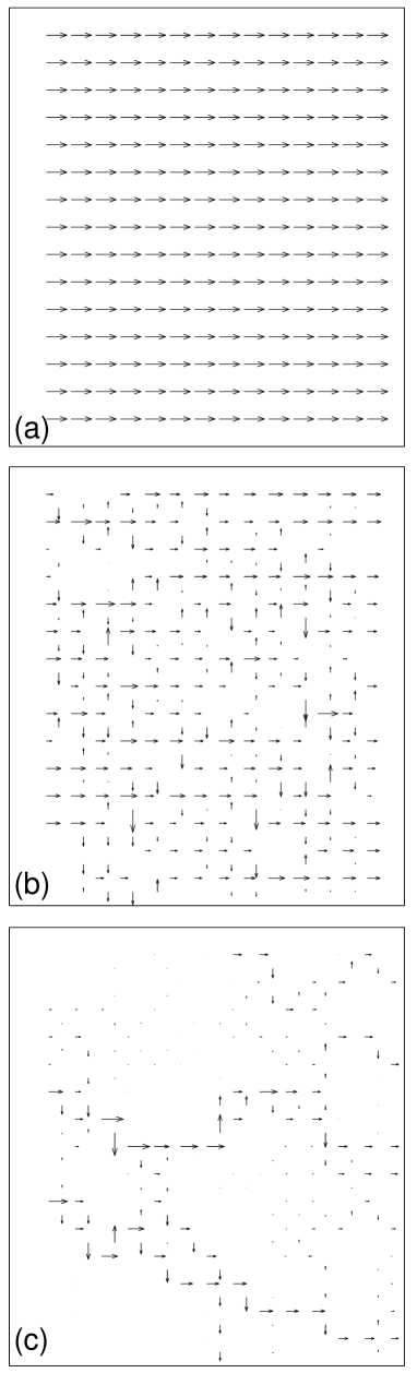
FIG. 1.: Calculated bond currents for a two-dimensional bond percolation model. The external voltage difference is applied between the left and right end sides of the network. The bond probabilities are $p=1$ (a), $p=0.8$ (b), and $p=0.55$ (c). The directions and sizes of the arrows represent the directions and the intensities of the bond currents, respectively.

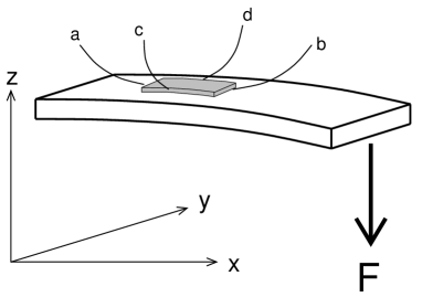
FIG. 2.: Schematical device for the measurement of the piezoresistive response. The cantilever beam is clamped at one end and a force $F$ acts downwards at the opposite end. The resulting strain field is transfered to the material of interest (dark region). The longitudinal response is obtained when a potential difference is applied between points a and b and the resulting conductance is measured for $F\neq 0$ and $F=0$. Instead, the transversal response is obtained when the potential difference is applied between c and d.

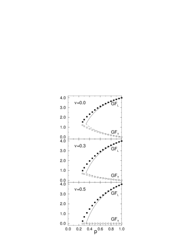
FIG. 3.: Longitudinal and tranversal gauge factors as a function of bond probability $p$ for different values of the Poisson ratio $\nu$. The tunneling probability has zero distribution ($\Delta K=0$) and $K=4$. Symbols refer to Monte carlo calculations (simple cubic lattice of $30\times 30\times 30$ sites) while the solid and dashed lines are the results of the effective medium approximation.

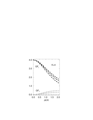
FIG. 4.: Longitudinal and tranversal gauge factors as a function of the tunneling distribution width $\Delta K$ for $K=4$ and $p=1$. From top to bottom: $\nu=0.0$, $0.3$, and $0.5$. Symbols and lines have the same meaning as in Fig. 3

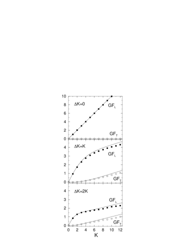
FIG. 5.: Longitudinal and tranversal gauge factors as a function of $K$ for $p=1$, $\nu=0.3$ and different values of the tunneling distribution width $\Delta K$. Symbols and lines have the same meaning as in Fig. 3

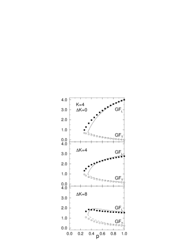
FIG. 6.: Longitudinal and tranversal gauge factors as a function of $p$ for different values of the tunneling distribution width $\Delta K$. $K=4$ and $\nu=0.3$. Symbols and lines have the same meaning as in Fig. 3

FIG. 7.: Factor of piezoresistive anisotropy $\chi$, Eq.(23), for the Monte Carlo results of Fig. 6.

REFERENCES

- [1] A. B. Pakhomov, X. Yan, and B. Zhao, Appl. Phys. Lett. 67, 3497 (1995).
- [2] N. F. Mott, J. Non-Cryst. Solids 1, 1 (1968); A. L. Efros and B. I. Shklovsii, J. Phys. C 8, 249 (1975).
- [3] B. Abeles, P. Sheng, M. D. Coutts, and Y. Arie, Adv. Phys. 24, 407 (1975).
- [4] P. Sheng and J. Klafter, Phys. Rev. B 27, 2583 (1983).
- [5] N. Savvides, S. P. McAlister, C. M. Hurd, and I. Shiozaki, Solid State Commun. 42, 143 (1982).
- [6] M.-C. Chan, A. B. Pakhomov, and Z.-Q. Zhang, J. Appl. Phys. 87, 1584 (2000).
- [7] N. M. White and J. D. Turner, Meas. Sci. Technol. 8, 1 (1997).
- [8] M. Prudenziati, Handbook of Sensors and Actuators (Elsevier, Amsterdam, 1994), p.189.
- [9] G. E. Pike and C. H. Seager, J. Appl. Phys. 48, 5152 (1977).
- [10] C. Canali, D. Malavasi, B. Morten, M. Prudenziati, and A. Taroni, J. Appl. Phys. 51, 3282 (1980).
- [11] The argument made in this qualitative discussion is general enough to leave the specific strain dependence of the bond conductances unspecified.
- [12] S. Kirkpatrick, Rev. Mod. Phys. 45, 574 (1973).
- [13] J. Bernasconi, Phys. Rev. B 9, 4575 (1974).
- [14] The same holds true also for .
- [15] C. Grimaldi, P. Ryser, and S. Strässler, cond-mat/0010181, preprint (2000). To appear on J. Appl. Phys.
- [16] I. S. Gradshtein and I. M. Ryzhik, Tables of Integrals, Series, and Prodicts (Academic, New York, 1963).