*

Abstract

The Euro ($EUR$) has been a currency introduced by the European Community on Jan. 01, 1999. This implies eleven countries of the European Union which have been found to meet the five requirements of the Maastricht convergence criteria. In order to test $EUR$ behavior and understand various features, we have extrapolated the $EUR$ backwards and therefore have obtained a false euro ($FEUR$) dating back to 1993. We have derived the exchange rates of the $FEUR$ with respect to several currencies of interest not belonging to the $EUR$, i.e., Danish Kroner ($DKK$), Swiss Franc ($CHF$), Japanese Yen ($JPY$) and U.S. Dollar ($USD$). We have first observed the distribution of fluctuations of the exchange rates. Within the Detrended Fluctuation Analysis ($DFA$) statistical method, we have calculated the power law behavior describing the root-mean-square deviation of these exchange rate fluctuations as a function of time, displaying in particular the $JPY$ exchange rate case. In order to estimate the role of each currency making the $EUR$ and therefore in view of identifying whether some of them mostly influences its behavior, we have compared the time-dependent exponent of the exchange rate fluctuations for $EUR$ with that for the currencies that form the $EUR$. We have found that the German Mark ($DEM$) has been leading the fluctuations of $EUR/JPY$ exchange rates, and Portuguese Escudo ($PTE$) is the farthest away currency from this point of view.

1 Introduction

The Euro ($EUR$) is a bona fide currency introduced by the European Community on Jan. 01, 1999 [1] in contrast to the $XEU$ which was a theoretical ”basket” of currencies. The $EUR$ is superseding national currencies in eleven countries of the European Union which have been found to meet the five requirements of the Maastricht convergence criteria [1]: price stability, fiscal prudence, successful European monetary system membership, and interest-rates convergence in particular. In order to test $EUR$ behavior and understand various features, we have extrapolated the $EUR$ backwards and therefore have obtained a false euro ($FEUR$) dating back to 1993. We have reconstructed the exchange rates of the $FEUR$ with respect to several currencies of interest not belonging to the $EUR$, i.e., Danish Kroner ($DKK$), Swiss Franc ($CHF$), Japanese Yen ($JPY$) and U.S. Dollar ($USD$). The $DKK$ is a currency for a country belonging to the European Community and outside the $EUR$ system. The $CHF$ is a European currency for a country NOT belonging to the European system. The $JPY$ and $USD$ are both major currencies outside Europe.

The irrevocable conversion rates of the participating countries have been fixed by political agreement based on various considerations and the bilateral market rates of December 31, 1998 [1, 2, 3]. Using these rates one false Euro ($FEUR$) can be represented as an unweighted sum of the eleven currencies $C_{i}$, $i=1,11$:

$$1EUR=\sum_{i=1}^{11}\frac{\gamma_{i}}{11}\,C_{i}$$ (1)

where $\gamma_{i}$ are the conversion rates and $C_{i}$ denote the respective currencies, i.e. Austrian Schilling ($ATS$), Belgian Franc ($BEF$), Finnish Markka ($FIM$), German Mark ($DEM$), French Franc ($FRF$), Irish Pound ($IEP$), Italian Lira ($ITL$), Luxembourg Franc ($LUF$), Dutch Guilder ($NLG$), Portuguese Escudo ($PTE$), Spanish Peseta ($ESP$). In order to study correlations in the $EUR$ exchange rates as of now, the $EUR$ existence can be artificially extended backward, i.e., before Jan. 01, 1999. This can be done by applying Eq.(1) to each participating currency for the time interval of the exchange rates which are available before Jan. 01, 99, thereby defining a more or less legal (but $false$) $FEUR$ before its birth. Nevertheless we drop the letter $F$ in $FEUR$ thereafter.

We are concerned with the behavior of $EUR$ toward currencies which are outside the European Union, since nowadays these are the only exchange rates of interest. These are e.g. Danish Kroner ($DKK$), Swiss Franc ($CHF$), Japanese Yen ($JPY$) and U.S. Dollar ($USD$). Therefore, we construct a data series of $EUR$ toward e.g. Japanese Yen ($EUR$/$JPY$) following the artificial rule:

$$1EUR/JPY=\sum_{i=1}^{11}\frac{\gamma_{i}}{11}\,C_{i}/JPY$$ (2)

However, the number of data points of the exchange rates for the period starting Jan. 1, 1993 and ending Dec. 31, 1998 is different for these eleven currencies toward $DKK$, $CHF$, $JPY$ and $USD$. This is due to different national and bank holidays when the banks are closed and official exchange rates are not defined in some countries. The number $N$ of data points has been equalized as done in [3], assuming that the exchange rate does not change if there is such a gap (usually a holiday), such that $N=1985$, spanning the interval time from January 1, 1993 till October 31, 2000.

The evolution of the $false$ (from Jan. 1, 1993 to Dec. 31, 1998) and the real (from Jan. 1, 1999 to Jun 30, 2000) $EUR$ with respect to the $DKK$, $CHF$, $JPY$, and $USD$ are plotted in Fig. 1. While the $EUR/DKK$ exchange rate is not much disturbed by the transition to the real $EUR$, the other currencies, in particular $USD$ and $JPY$ and a little bit less $CHF$ have been much sensitive to the transition.

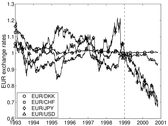
Figure 1: Normalized evolution assuming an exchange rate = 1 on Jan. 01, 1999 for $EUR/DKK$, $EUR/CHF$, $EUR/JPY$ and $EUR/USD$

The $DFA$ technique [4] has been often described and is not recalled here. It leads to investigating whether the root-mean-square deviations of the fluctuations of the investigated signal $y(n)$ has a scaling behavior, e.g. if the function $<F^{2}(\tau)>$ scales with time as

$$\langle{1\over\tau}{\sum_{n=k\tau+1}^{(k+1)\tau}{\left[y(n)-z(n)\right]}^{2}}\rangle\sim\tau^{2\alpha}$$ (3)

where $z(n)$ is hereby a linear function fitting at best the data in the $\tau$ interval which is considered. A value $\alpha=0.5$ corresponds to a signal mimicking a Brownian motion.

Let it be recalled that in [3] it has been shown that the time scale invariance for $EUR/CHF$, $EUR/USD$, and $EUR/JPY$ holds from 5 days (one week) to about 300 days (one year) showing Brownian type of correlations. Two different scaling ranges were found for the $EUR/DKK$; one, from four to 25 days (5 weeks) with a non-Brownian $\alpha=0.37\pm 0.01$, and another, after that for up to 300 days (61 weeks) with Brownian-like correlations.

In order to estimate the role of each currency making the $EUR$ and therefore in view of identifying whether some of them mostly influences its behavior, we have first looked at the distribution of exchange rate fluctuations in the interesting time interval defined above. Next the time-dependence of the $\alpha$ exponent characterizing the scaling law for the exchange rate fluctuation correlations for $EUR$ and that for the 11 currencies that form $EUR$ has been calculated. This evolution has been averaged (i) over the currencies, (ii) over the time interval considered here. The results are compared here to the behavior of the fluctuation correlations for $EUR/JPY$ and $DEM/JPY$ exchange rates. Let it be pointed out that we have also tested elsewhere the $DKK$, $CHF$ and $USD$ exchange rates with respect to $EUR$, $DEM$ and the other $EUR$ forming currencies [5].

2 Distribution of the fluctuations and strong currency

It is of interest to observe whether the usual statement that the $EUR$ is nothing else than a generalized $DEM$ holds true. In order to do so we have first compared the distributions of the exchange rate fluctuations for $DEM/DKK$, $DEM/CHF$, $DEM/JPY$, $DEM/USD$ with the distributions of the fluctuations for $EUR/DKK$, $EUR/CHF$, $EUR/JPY$, $EUR/USD$ (Fig. 2). From such a comparison we are led to consider that $DEM$ is dominant in defining the distribution of the fluctuations of $EUR$ exchange rate with respect to $DKK$, $CHF$, $JPY$ and $USD$. For all cases the central part of the distributions can be fitted by a Gaussian distribution while the tails, i.e. the large fluctuations, follow a power law with a slope equal to $ca.$ 2.9 for $EUR/CHF$ and $DEM/CHF$, 3.2 for the negative and 4.0 for the positive tail of $EUR/JPY$ and $DEM/JPY$, and 3.2 for the negative and about 4.5 for the positive tail in $EUR/USD$ and $DEM/USD$.

It is fair to recall that the volatility of exchange rates follows different scaling laws depending on the horizon which is considered [6]. However the correlation coefficient stabilizes at scales one day and higher [7]. Those values might be examined whether they result from the equivalent of trading momentum and price resistance just like in the model of [8] for stock price and price fluctuation distribution. The above asymmetry in the power law for the positive and negative tail might result or not from the limited amount of data.

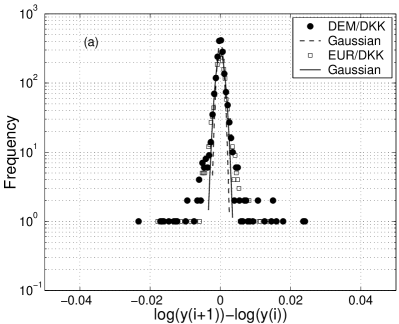
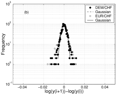
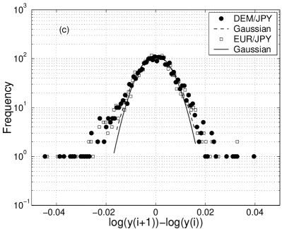
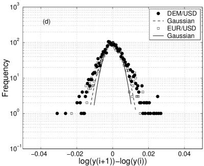
Figure 2: The distribution of the fluctuations of (a) $DEM/DKK$ and $EUR/DKK$, (b) $DEM/CHF$ and $EUR/CHF$, (c) $DEM/JPY$ and $EUR/JPY$, and (d) $DEM/USD$ and $EUR/USD$, as compared to the Gaussian distribution. Dashed lines correspond to a Gaussian fit to the $DEM$ exchange rate distributions while solid lines represent a Gaussian fit to the $EUR$ exchange rate distributions

3 Correlations of the fluctuations and strong currency

As done elsewhere [9], in order to probe the existence of locally correlated and decorrelated sequences, we have constructed an observation box, i.e. a 515 days ($\simeq$ 2 years) wide window probe placed at the beginning of the data, calculated $\alpha$ for the data in that box, moved this box by one day toward the right along the signal sequence, calculated $\alpha$ in that box, a.s.o. up to the $N$-th day of the available data. A local, time dependent $\alpha$ exponent is thus found for the $N-515$ last days. The $JPY$ exchange rate case results only are illustrated in this report. The time dependent $\alpha$-exponent for $EUR/JPY$ and that for each of the 11 currency (which form the $EUR$) exchange rates toward $JPY$ have been computed. Together with the $EUR/JPY$ result, some of the time dependent $\alpha$-exponents, i.e. for $ATS/JPY$, $DEM/JPY$, $ITL/JPY$, $PTE/JPY$ are shown in Fig. 3 as the most representative ones of various behaviors. Notice, the similarity between $EUR/JPY$ and $DEM/JPY$, a maximum in 1998 but a rather flat behavior for $ATS/JPY$, a very irregular behavior for $ITL/JPY$, and an increase in $\alpha$ around 1998 for $PTE/JPY$. The other cases, i.e. $BEF/JPY$, $FIM/JPY$, $FRF/JPY$, $IEP/JPY$, and $NLG/JPY$ are similar to $ATS/JPY$ and $DEM/JPY$ cases. While the differences in the $\alpha$-behavior after Jan. 1, 1999 are almost undistinguishable, the time dependent $\alpha$-exponents before that day exhibit nevertheless different correlated fluctuations depending on the currency. We stress that $\alpha$ for $EUR/JPY$ most closely resembles the $DEM/JPY$ before and after Jan. 01, 99, they are almost identical already since mid 1996.

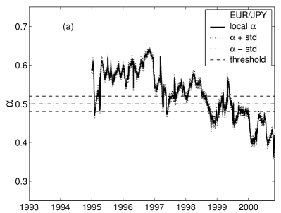
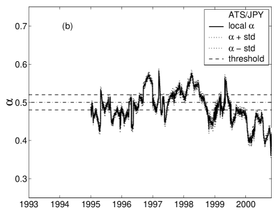
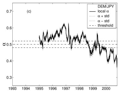
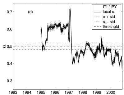
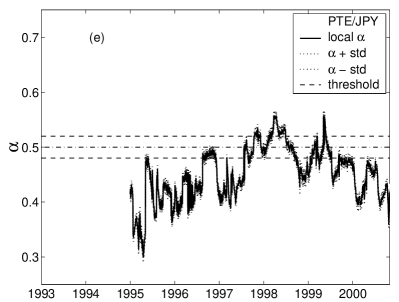
Figure 3: The evolution of the local value of $\alpha$ estimated with the $DFA$ method for a window of size 2 years (solid line) for (a) $EUR$, (b) $ATS$, (c) $DEM$, (d) $ITL$, (e) $PTE$ with respect to $JPY$. Dotted lines mark one standard deviation in the $\alpha$ estimate. Dashed horizontal lines indicate a 0.02 threshold relative to the uncorrelated fluctuations of a Brownian motion signal, $\alpha=0.5$

Notice that the $\alpha$-exponent for $EUR/JPY$ and those $\alpha$-values of the other currency exchange rates are not strictly equal to each other even after Jan. 1, 1999 because the fit window used for calculating $\alpha$ includes days prior to Jan. 1, 1999. A strict identity should only occur on Jan. 1, 2001, i.e. after two years (515 days) from $EUR$ strict birth. Yet, the values are already very close to each other (less than 1%) before such a date.

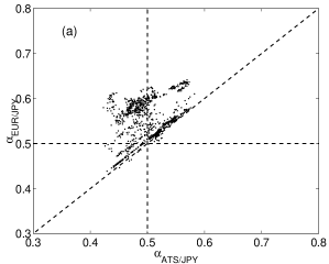
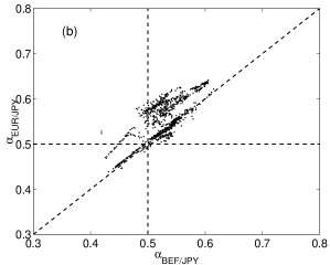
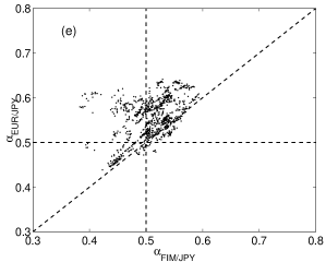
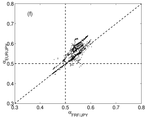
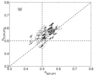
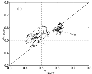
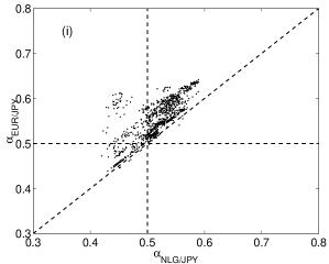
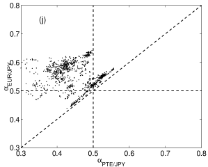
Figure 4: Structural correlation diagram of the $DFA$ - $\alpha$ exponent for the exchange rate $EUR/JPY$ and the $DFA$ - $\alpha$ exponent for the exchange rate with respect to $JPY$ of the 11 currencies forming one $EUR$; ($BEF$=$LUF$)

Looking for more diversified answers to our question on whether e.g. $DEM$ truly controls the market, we have constructed a graphical correlation matrix of the time-dependent $\alpha$ exponent for the various exchange rates of interest. In Fig. 4(a–j), the correlation matrix is displayed for the time interval between Jan. 1, 1993 and Jan. 1, 1999 for $\alpha_{EUR/JPY}$ vs. $\alpha_{C_{i}/JPY}$, where $C_{i}$ stands for the 11 currencies that form the $EUR$; ($BEF$=$LUF$). As described elsewhere, e.g. in [10], such a diagram can be divided into sectors through a horizontal, a vertical and perpendicular diagonal lines crossing at (0.5,0.5). If the correlation is strong the cloud of points should fall along the slope $=1$ line. This is clearly the case of the relationship between $\alpha_{EUR/JPY}$ and $\alpha_{DEM/JPY}$, while the largest spread is readily seen for $\alpha_{EUR/JPY}$ $vs.$ $\alpha_{PTE/JPY}$.

In order to assess additional features of the time dependent $\alpha$-exponents of the exchange rate fluctuation correlations we have time averaged $\alpha$ for the $EUR$ exchange rate with respect to $JPY$, and for each of the 11 eleven currencies which form $EUR$, over the time interval [Jan. 1, 1993 - Jan. 1, 1999]. We present the results of $\alpha_{mean}$, $\alpha_{median}$, $\alpha_{mean}/\alpha_{median}$ and the standard deviation $\sigma(\alpha)$ in Table I. The time evolution of such quantities is given in Figs. 5(a–d), where $\alpha_{mean}-\alpha_{median}$ rather than $\alpha_{mean}/\alpha_{median}$ is displayed for readability.

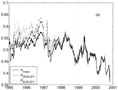
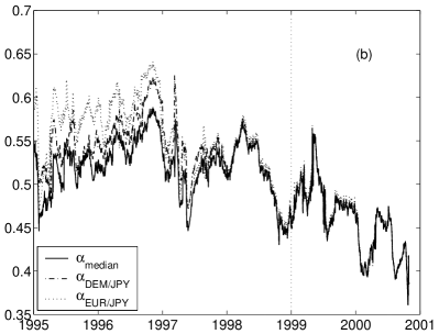
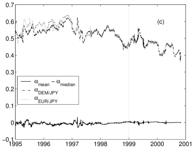
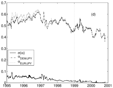
Figure 5: Time dependent mean, median, mean-median and standard deviation of the $\alpha$-exponents resulting from the time dependent $\alpha$ distributions of the eleven currencies that form the $EUR$ and the corresponding time dependent quantities of the $\alpha$-exponents for $EUR/JPY$ and $DEM/JPY$

Several remarks follow from the correlations shown with the structural diagrams and the relations between the $\alpha_{mean}$ and $\alpha_{median}$. While the structural diagrams for $ATS$, $PTE$, and $ITL$ with respect to $EUR$ show weak or no correlation at all, the $\alpha_{mean}$ is equal within the error bars to the $\alpha_{median}$ for $PTE$ and $ATS$ but $\alpha_{mean}$ and $\alpha_{median}$ are markedly different from each other for $ITL$. On the other hand, $\alpha_{mean}$ is not equal to $\alpha_{median}$ for $DEM$ but the structural diagram shows very strong correlations between the time dependent $\alpha$-exponents. It is clear that the leading currencies from the point of view of the exchange rate fluctuations were $DEM$, and to a lesser extent $BEF$, $FRF$, $IEP$, and $NLG$ while $PTE$ is far away from the main stream, i.e. $\alpha\simeq 0.45$. We stress the quite small and quite large values of $\sigma(\alpha)$ for $ATS$ and $ITL$ respectively, both having the largest $\alpha_{mean}/\alpha_{median}$ ratio, both greater than unity in fact, indicating e.g. specific national bank financial policies.

Let it be pointed out that $\alpha_{mean}$ follows $\alpha_{EUR/JPY}$ while $\alpha_{median}$ follows the fluctuations of $\alpha_{DEM/JPY}$.

Table 1: Averaged values for the time interval [Jan. 1, 1993 ; Jan. 1, 1999] of the time dependent $\alpha$-exponents of the exchange rate with respect to the Japanese Yen ($JPY$) for $EUR$ and those 11 currencies forming the $EUR$ on Jan. 01, 99.

Currency	$\alpha_{mean}$	$\alpha_{median}$	$\alpha_{mean}$/$\alpha_{median}$	$\sigma(\alpha)$
EUR	0.5541	0.5565	0.9956	0.0441
ATS	0.4994	0.4971	1.0046	0.0355
BEF	0.5264	0.5284	0.9961	0.0357
DEM	0.5389	0.5408	0.9966	0.0361
ESP	0.5076	0.5062	1.0028	0.0398
FIM	0.5096	0.5136	0.9922	0.0388
FRF	0.5366	0.5408	0.9923	0.0325
IEP	0.5282	0.5339	0.9893	0.0395
ITL	0.5348	0.5174	1.0337	0.0763
LUF	0.5264	0.5284	0.9961	0.0357
NLG	0.5168	0.5200	0.9937	0.0364
PTE	0.4483	0.4440	1.0097	0.0534

4 Conclusion

We have thus studied a few aspects of the $EUR$ exchange rates from the point of view of the fluctuations of the $EUR$ and the 11 currencies forming the $EUR$. We have examined here the exchange rates toward $DKK$, $CHF$, $JPY$ and $USD$. The central part of the distribution of the fluctuations can be fitted by a Gaussian, while the distribution of the large fluctuations follows a power law. We have observed that the $DEM$ is the strongest currency that has dominated the correlations of the fluctuations in $EUR$ exchange rates with respect to $JPY$, while $PTE$ was the most extreme one in the other direction.

Acknowledgements

We are very grateful to the organizers of the Symposium for their invitation. We gratefully thank the Symposium sponsors for financial support.

References

- [1] http://pacific.commerce.ubc.ca/xr/euro/
- [2] http://pacific.commerce.ubc.ca/xr/euro/euro.html#Rates
- [3] Ausloos M., Ivanova K. (2000) Introducing False and false exchange rates. Physica A 286:353
- [4] Peng C.-K., Buldyrev S.V., Havlin S., Simmons M., Stanley H.E., Goldberger A.L. (1994) On the mosaic organization of DNA sequences. Phys Rev E 49:1685
- [5] Ausloos M., Ivanova K. (2001) Correlations Between Reconstructed Exchange Rates vs. , , , and . Int J Mod Phys C (in press)
- [6] Friedrich R., Peincke J., Renner Ch. (2000) How to quantify deterministic and random influences on the statistics of the foreign exchange market. Phys Rev Lett 84:5224
- [7] Gencay R., Selcuk F., Whitcher B. (2001) Scaling properties of foreign exchange volatility. Physica A 289:249
- [8] Castiglione F., Pandey R. B., Stauffer D. (2001) Effect of trading momentum and price resistance on stock market dynamics: a Glauber Monte Carlo simulation. Physica A 289:223
- [9] Vandewalle N., Ausloos M. (1997) Coherent and random sequences in financial fluctuations. Physica A 246:454
- [10] Ausloos M., Ivanova K. (2001) False Euro () exchange rate correlated behaviors and investment strategy. Eur Phys J B (in press)