Evolution of the stripe phase as a function of doping
from a theoretical analysis of angle-resolved photoemission data

Abstract

By comparing single-particle spectral functions of $t$-$J$ and Hubbard models with recent angle-resolved photoemission (ARPES) results for LSCO and Nd-LSCO, we can decide where holes go as a function of doping, and more specifically, which type of stripe (bond-, site-centered) is present in these materials at a given doping. For dopings greater than about 12% our calculation shows furthermore that the holes prefer to proliferate out of the metallic stripes into the neighboring antiferromagnetic domains. The spectra were calculated by a cluster perturbation technique, for which we present an alternative formulation. Implications for the theory for high-T_c superconductivity are discussed.

I Introduction

At present, stripes are at the heart of the debate concerning the mechanism of superconductivity in high-temperature superconductors (HTSC). There is clear experimental evidence for static stripes in Nd-doped LSCO (Nd-LSCO, for example La_1.48Nd_0.4Sr_0.12CuO₄) from elastic neutron scattering experiments [1]. The existence of a dynamical stripe phase in the “real” high-T_c compound LSCO or even in YBCO has been conjectured from similar diffraction patterns in the inelastic neutron scattering results [2, 3]. However, it has not been decided so far, whether the observed pattern is due to one-dimensional spin-inhomogeneities (i.e. stripes) [2] or to two-dimensional incommensurable spin-waves [4]. In the case of YBCO near optimal doping, it has been suggested that the incommensurable fourfold neutron scattering peak is due to the dispersion of the famous 41meV commensurable (found below T_c at momentum ${\bf k}=(\pi,\pi)$) neutron scattering peak to lower excitation energies around ${\bf k}=(\pi,\pi)$ [4]. From the theoretical point of view, several numerical analyses, ranging from Hartree-Fock [5, 6], DMRG [7] to dynamical mean-field theory [8] indicate that stripes can be produced by purely strong-correlation effects. On the other hand, structural transformations [1, 9, 10] as well as long-range Coulomb interactions [11, 12] may also play an important role in the formation of stripes.

In this article, we provide numerical arguments showing that an essential link in the chain of evidence for stripes is provided by angle-resolved photoemission spectroscopy (ARPES): ARPES spectra show hardly any difference between LSCO (dynamical stripes candidate) and Nd-LSCO (static stripe system) [13, 14, 15]. This fact was first pointed out by a semiphenomenological argument by Salkola et al. [16]. In a previous paper, we have shown that salient spectral features of Nd-LSCO and LSCO can be explained by a model with static stripes [17]. Here, we will show that the spectra of LSCO and Nd-LSCO can be almost quantitatively described by different types of stripe states (i.e. site-centered, bond-centered) for a wide variety of dopings. Since the experimental ARPES spectra for LSCO and Nd-LSCO are so similar and their spectra can be quantitatively described by stripe models, we argue that there must be stripes present in LSCO as well, at least in the underdoped to optimally doped regime.

If stripes are present as low-energy excitations in the high-T_c compounds, they must affect the microscopic description of the superconducting state, independently on whether they are an obstacle against superconductivity or even its driving force. In this context, an important question is, whether stripes are bond-centered or site-centered since, theoretically, bond-centered stripes have been shown to enhance superconducting pairing correlations [18, 12]. By analyzing the different scenarios with our technique and comparing the results with ARPES spectra for different dopings, we can decide which type of stripe (bond- or site-centered) better describes the spectrum as a function of doping.

Very recently, Zhou et al. [14] succeeded in measuring ARPES data on Nd-LSCO and LSCO systems with different doping levels. In the doping region beyond 12% the ARPES results reveal a dual nature of the electronic structure: The straight segments forming the “Fermi surface” in energy-integrated photoemission and the $(\pi,0)$ low-energy excitations, which have been attributed to site-centered stripes for the 12% doping case [17], are still present but overlaid with more two-dimensional (2D) features reminiscent of a simple tight-binding band-structure for homogeneous 2D systems. Zhou et al. address the experimental question, whether the two features originate from the mixing of two different phases or whether they are intrinsic properties of the same stripe phase. In the first case (phase separation) there should a non-stripe phase with a very high carrier concentration (as estimated from the area inside the Fermi surface) coexisting with a phase of site-centered stripes. The authors remark that there is hardly evidence for such a phase in Nd-LSCO and LSCO at the doping levels under consideration [15, 19]. Another scenario consistent with the experimental observation would be that the system forms more and more bond-centered stripes upon increasing the doping beyond 12%. The possibility for the latter scenario was already indicated by our earlier calculations [17], where the spectrum of bond-centered stripes resembles the diamond-shaped two-dimensional feature observed by Zhou et al.. In the present article we will show that the evolution of the experimental ARPES with increasing doping can be described by assuming that more and more bond-centered stripes are formed at the expense of site-centered ones (as conjectured previously by Zhou et al.).

Our approach adopts the Cluster-Perturbation-Theory (CPT) developed by Senechal et al. [20], which consists in splitting the infinite lattice into clusters which are treated by exact diagonalization. The inter-cluster hopping terms are then treated perturbatively, so that one eventually approximates the infinite lattice. This method takes into account exactly the local correlations, which probably are the most important ones in these systems, and at the same time makes all $k$ points of the Brillouin Zone available. In addition, this is an ideal method to deal with a “larger unit cell” such as the one present in the stripe phase. One should, however, mention that, at this level, the method is not appropriate to explore stripe stability for a given model. As a matter of fact, this is not the aim of the present work. Rather, via this CPT approach we enforce a stripe pattern by connecting clusters with different hole dopings [see Fig. (4)], and study its spectral function to compare with ARPES experiments. A similar approach has been taken in Ref. [21], where the hole spectral function for site-centered stripe patterns was calculated within the string picture.

Our paper is organized as follows: In section II, we explain in detail how the CPT is applied to the stripe phase. In section III our numerical results are presented and compared with ARPES spectra. The content of this article is summarized in section IV. Finally, the appendix presents an alternative derivation of the CPT equation, by means of a mapping onto a hard-core fermion model. In this appendix, we show that the CPT approximation amounts to neglecting two-particle excitations within this model.

II Technique

The computational technique for our calculation of the single-particle spectral weight $A({\bf k},\omega)$ and for the Green’s function is a special application of the CPT for inhomogeneous systems. This method is based on a strong-coupling perturbation expansion of the (Hubbard model’s) one-body hopping operators linking the individual unit-cells [20]. At lowest order in this expansion, the Green’s function of the infinite lattice can be expressed (in matrix form) as:

$$G^{\infty}({\bf P},z)=\frac{G^{cluster}(z)}{1-\epsilon({\bf P})G^{cluster}(z)}\;,$$ (1)

where the matrices $G^{\infty}$, $G^{cluster}$, and $\epsilon({\bf P})$ will be defined around Eq. (2). The authors of ref.[20] have pointed out that the above formula becomes exact in the limit of vanishing interaction ($U/t=0$) and, obviously, in the atomic limit ($t=0$), and can thus be considered as an interpolation scheme between $t\rightarrow\infty$ and $t\rightarrow 0$. Notice, however, that this formula does not become exact in the $U\to\infty$ limit. In the interesting regime where the interaction and the hopping are of the same order of magnitude Sénéchal et al. have shown numerically that Eq.(1) gives as an accurate interpolation between the two limiting cases. Additionally, we have shown in our previous article [17] that the cluster perturbation technique is ideally suited to study inhomogeneous systems such as the stripe state in the high-T_c compounds.

In order to deal with stripes, the infinite lattice is divided into unit cells of equal size (Fig.(1a)). The unit cell is further divided into independent blocks to incorporate the stripe topology: In the example of Fig.(1), we are interested in a site-centered (“3+1”) configuration with quarter-filled metallic chains alternating with half-filled 3-leg ladders. The 3-leg ladders (here $3\times 6$ blocks) and quarter-filled chains (here $1\times 12$ with 6 holes, see Fig.(1b)) are solved by exact diagonalization, yielding the single-particle spectral function of the block. The individual Green’s functions of the blocks forming a unit-cell cluster are combined to form the Green’s function of the unit cell $G^{cluster}$ at “order zero”, i. e., in which the intra-cluster hopping terms are set to zero. In a second step, the intra-cluster hopping connecting the individual blocks both within the same unit cell and in different unit cells (dashed lines in Fig.(1b)) are incorporated via the cluster perturbation technique. This yields the desired Green’s function of the infinite lattice. Where it was technically feasible, we doubled the unit cell (as in Fig.(1)) and diagonalized two 3-leg ladders with a staggered magnetic field pointing in opposite directions, resulting in a $\pi$-phase shifted (between the AF domains) Néel order in the final configuration. This site-centered “$3+1$” configuration with $\pi$-phase shifted Néel order of stripes was first suggested by Tranquada et al. [1]. Bond-centered stripes, on the other hand, are modeled by 2-leg ladders with alternating filling. In the following, we will refer to this bond-centered configuration as “$2+2$”.

Holes can propagate out of the metallic stripes into the AF insulating domains via the inter- and intra-unit-cell hoppings (dashed lines in Fig.(1)). As explained above, our method consists in “forcing” the stripe structure “by hand” in order to study the effects of this structure on the photoemission spectrum. The different hole concentration in the “metallic” and in the “antiferromagnetic” region is achieved by adjusting independently the chemical potential of the individual blocks so that the desired hole density (see Fig. 4) is obtained. This corresponds to introducing an on-site energy shift between the two blocks $\Delta\approx 1.5t$. Physically, this shift corresponds to the energy of the stripe formation, possibly produced by a combined effect of strong correlation and of lattice distortion occurring in the low-temperature tetragonal (LTT) phase [1]. Of course, without such an energy shift it would be impossible to obtain such large density oscillations, such as the ones shown in Fig. 4. Indeed, in a homogeneous system the amplitude of charge oscillations remains of the order or less than $0.1$, as shown, e. g., by DMRG calculations[7, 12].

Alternatively equation(1) can be obtained by expressing the fermionic creation/annihilation operator $c^{(\dagger)}_{i}$ in terms of fermionic creation and annihilation operators $d^{(\dagger)}_{\alpha}$ representing the photoemission and inverse photoemission target states $|\alpha\rangle$ of the diagonalized cluster. This derivation of Eq. (1) is presented in the appendix.

In Eq. (1), ${\bf P}$ is a superlattice wave vector and $G^{\infty}$ is the Green’s function of the “$\infty$-size” 2D system, however, still in a hybrid representation: real space within a cluster and Fourier-space between the clusters. This is related to the fact that $G^{\infty}({\bf P},z)$ is now an $M\times M$ matrix in the space of site indices (in the inhomogeneous stripe configuration of Fig.(1b) $M=2\times(3\times 6)+1\times 12=96$). Likewise, $\epsilon({\bf P})$ and $G^{cluster}$ are $M\times M$ matrices in real space with $\epsilon({\bf P})$ standing for the perturbation. For the situation in Fig.(1b), the only nonzero elements of the hermitian matrix $\epsilon({\bf P})$ are represented by the dashed bonds in the figure:

$$\epsilon({\bf P})_{l,m}=\left\{\begin{array}[]{r@{\quad:\quad}l}-t&\mbox{dashed bonds inside cell}\\ -te^{\pm iP_{x/y}}&\mbox{bonds connecting cells}\\ 0&\mbox{elsewhere}\end{array}\right.\;.$$ (2)

In order to facilitate diagonalization of the individual clusters, we used periodic boundary conditions along the stripe direction. In principle, this introduces hopping terms, which are not present in the infinite lattice. However, this is not a problem, since these terms can be consistently removed perturbatively by subtracting corresponding terms to the matrix elements of $\epsilon({\bf P})$.

A complete Fourier representation of $G^{\infty}$ in terms of the original reciprocal lattice then yields the cluster perturbation theory (CPT) approximation [20].

To allow for larger block sizes, we actually diagonalized the $t$-$J$ model on the blocks to obtain the (block-) Green’s functions as an approximation for the Hubbard model’s (block-) Green’s function. The $t$-$J$ Hamiltonian is defined as

$$H=-t\sum_{\langle i,j\rangle,\sigma}(\hat{c}^{\dagger}_{i,\sigma}\hat{c}_{j,\sigma}+\mbox{h.c.})+J\sum_{\langle i,j\rangle}({\bf S}_{i}{\bf S}_{j}-\frac{n_{i}n_{j}}{4}).$$ (3)

The sums run over all nearest neighbor pairs $\langle i,j\rangle$. No double occupancy is allowed. We have chosen the commonly accepted values $J/t=0.4$ and $t\approx 0.5eV$.

The quality of this approximation is tested by comparing single-particle spectral functions of 2+2 bond-centered stripe configurations at 12% doping based on diagonalizations of both Hubbard- and $t$-$J$ models. In Fig.(2), we show $A(\vec{k},\omega)$ for the standard walk through the Brillouin zone. One observes that the result for the Hubbard model ($U=8t$, Fig. (2a)) is very similar to the $t$-$J$ model result ($J=0.4t$, Fig.(2b)): The dispersion is two-dimensional, metallic-like and comparable to a tight-binding dispersion. The only difference between the figures is quantitative, namely, the different Fermi velocities and bandwidths. This difference is predominantly due to the omission of the conditional hopping terms $\sim J$[22] in the $t$-$J$ Hamiltonian. Another reason may be due to the fact that the basic parameters of the models, the interaction strengths $J$ and $U$ have not been fine-tuned to match each other. The integrated spectral weight obtained from the two models is depicted in Fig.(3). In both cases, the occupation in momentum space $n(\vec{k})$ is distributed almost isotropically around the $\Gamma$ point. The low-energy excitations for both models indicate a two-dimensional LDA-like Fermi surface, however with additional weight at the $(\pm\pi,0)$, $(0,\pm\pi)$ points. The additional $(\pi,0)$ features are sharper in the Hubbard-model case.

Turning on the perturbation allows the holes to travel between the blocks and unit-cells. In Fig.(5), we show the electron concentration (averaged in the direction along the stripes) in the direction perpendicular to the stripes before (thick lines) and after (bars) applying CPT for the stripe configurations that are discussed in this article. As can be seen, the holes do not travel far from the domains that were originally defined, and the electron occupation hardly changes from the unperturbed setup. Therefore, the desired stripe configuration is conserved in our approach.

III Numerical results

We proceed to the discussion of the spectra for the underdoped region: At 10 % doping, the stripes have a charge periodicity of 5 lattice constants according to the Tranquada picture. This configuration has been modeled by a $5\times 12$ unit cell consisting of two half-filled $4\times 6$ systems (stacked on top of each other) and a quarter-filled 12-site chain as displayed in Fig.(4a). Fig.(6a) shows that the spectral weight is confined in one-dimensional segments of the Brillouin zone indicating a one-dimensional Fermi surface. The low-energy excitations in Fig.(7a) are mainly located at the $(\pm\pi,0)$ and $(0,\pm\pi)$ points in momentum space. In Fig.(8a) the single-particle spectral function for this doping is plotted directly and one observes the characteristic stripe features that have been discussed in detail in [17]: a dispersionless band near $(\pi,0)$ crossing the Fermi surface at $(\pi,\pi/4)$ resulting from the one-dimensional chain oriented in $y$-direction, the double-peak structure at $(\pi,0)$ from the hybridization of the metallic band with the top of the antiferromagnetic band and an excitation at $(\pi/2,\pi/2)$ at higher binding energies than at $(\pi,0)$. The combined results for this doping agree very well with the recent ARPES results by Zhou et al. [14] giving further support for the static stripe picture by Tranquada: at least below 12% doping, charge carriers are only present in quarter-filled chains that are alternating with half-filled antiferromagnetic domains and an increasing of doping is realized by lowering the distance between the chains and therefore reducing the effective size of the antiferromagnetic domains.

The incommensuration of the quasi-elastic Neutron scattering does not increase any more beyond a doping level of 12%. The simple picture of one-dimensional chains moving closer together at the expense of antiferromagnetic undoped domains thus cannot be valid in this regime. For a doping of $1/8$, we have previously shown[17] that the ARPES data can be explained by assuming that the static stripe system (Nd-LSCO) is in a state of site-centered stripes, where 3-leg antiferromagnetic ladders alternate with quarter-filled chains. Here we will address the question how to describe the system for dopings higher than $1/8$ or 12%.

The ARPES results by Zhou et al. suggest that LSCO and Nd-LSCO samples at 15 % doping are in a state that is still mainly in a 3+1 stripe phase since the ARPES results show all the features that have been previously observed for the $x=0.12$ samples: one-dimensional Fermi surface and low energy excitations located at $(\pm\pi,0)$ and $(0,\pm\pi)$. In addition, however, low-energy excitations appear around the edge of a diamond located at the center of the Brillouin zone. These excitations are connecting the $(\pi,0)$ features. Zhou et al. conjecture that bond-centered stripes are formed at the expense of site-centered ones, since it was shown in our previous calculation that bond-centered stripes do indeed exhibit such a diamond-shaped low-energy excitation pattern. This description is particularly interesting since bond-centered stripes in contrast to site-centered ones have been shown to enhance superconducting pairing correlations [18]. Therefore, this picture may provide a link to the doping dependence of the superconducting transition temperature of LSCO. However, to be able to relate bond-centered stripes to the diamond-shaped low-energy excitations that appear in LSCO and Nd-LSCO at 15 % doping, one has to study bond-centered stripes at higher dopings than $x=15\%$, since, in a phase-separated state, they have to carry all the additional holes that make up the overall doping of $x=15\%$ of the experimental sample. Here, we study three possibilities of “overdoped” stripe configurations as displayed in Fig.(4) (labeled b,c,d consistent with the figure label of Ref. [14]):

b) 2+2 bond-centered configuration (AF doped), Fig.(4b): Here, one ladder is at the filling $\langle n\rangle=0.75$ as in the case of 12% doping and the other ladder (previously undoped in the 12% doping case) with a filling of $\langle n\rangle=0.875$ yielding an overall doping of 19 %. In this scenario the doped region extends into the antiferromagnetic domain between the charged stripes. Technically, this configuration has been realized by coupling a $2\times 8$ ladder (2 holes) with a $2\times 8$ ladder (4 holes).

c) 2+2 bond-centered configuration, Fig.(4c): Here, one ladder is at the filling $\langle n\rangle=0.625$ and the other ladder stays half-filled as in the 12% doping case, again yielding an overall doping of 19 %. In this scenario the excess holes further populate the charged stripe. Technically, this configuration has been realized by coupling a $2\times 8$ ladder (no holes) with a $2\times 8$ ladder (6 holes).

d) 3+1 site-centered configuration, Fig.(4d): Here, the chain is quarter-filled ($\langle n\rangle=0.5$) as in the case of 12% doping and the three-leg ladder (previously undoped in the 12% doping case) has a filling of $\langle n\rangle=0.89$ yielding an overall doping of 21 %. In this scenario, the doped region extends into the antiferromagnetic domain between the charged stripes (as in case b). Technically, this configuration has been realized by coupling two $3\times 6$ ladders (2 holes each) with a $1\times 12$ chain (6 holes).

In Fig.(6 b,c,d) the electron occupation in momentum space is displayed. Neither of the three configuration shows the typical stripe signatures (one-dimensional distribution of spectral weight) but the weight is more or less isotropically distributed around the $\Gamma$-point. The spectral weight in Fig.(6 c) is almost circularly distributed and resembles $n(\vec{k})$ of the free electron gas. The weight distribution in Figs. (6 b,d), on the other hand, is more of a diamond shape. In the “phase-separated” picture, we expect the spectral weight stemming from the above configurations (b,c,d) to be superimposed onto the spectral weight coming from the dominating 3+1 site-centered structure which is all concentrated in the one-dimensional segments in momentum space. This might be the reason that in the actual experiment Zhou and coworkers can only resolve the latter.

For the low-energy excitations, the situation is different since a much smaller energy window is integrated and therefore the experiment is more sensitive to smaller amounts of spectral weight: Here, the results of the calculation are shown in Figs. (7 b,c,d). The low-energy excitations of the 2+2 configuration c are concentrated around the $(\pm\pi/2,\pm\pi/2)$ points. Overlaying these excitations with the 3+1 site-centered features would not yield the experimentally observed diamond structure connecting the $(\pi,0)$ excitations and therefore this configuration can be discarded. In contrast, the other 2+2 configuration b, where the extra holes are populating the antiferromagnetic domains does indeed show the experimentally observed diamond shape. In this setup, the $(\pi,0)$ features are present as well. They further enhance the low-energy excitations in this region of momentum space which are due to the domains that are still in the 3+1 site-centered configuration (present at 12% doping). The doped 3+1 site-centered configuration d, where the holes extend into the antiferromagnetic region also has its low-energy excitations distributed around a diamond centered at the $\Gamma$ point (Fig. (7 d). However, its features are not as sharp as in Fig.(7 b). This configuration cannot be so easily discarded and might be present in the actual material.

For completeness, we display the single-particle spectral weight of the three “overdoped” stripe configurations in Figs. (8 b,c,d): Configurations b and d show a two-dimensional tight-binding-like dispersion, the difference being the large amount of spectral weight that is concentrated near the Fermi level at $(\pi,0)$ for the bond-centered configuration b, which was also visible in the low-energy excitation plot (Fig.(7 b)). The other bond-centered configuration c, where all doped holes are concentrated in one ladder, only has a Fermi-level crossing at $(\pi/2,\pi/2)$ (“hole-pockets”) consistent with Fig.(7 c).

IV conclusion

In this work, the cluster perturbation technique and its application to the stripe phase of high-T_c materials and related compounds has been studied in detail. The CPT has been applied to Hubbard and $t$-$J$ systems with different dopings and stripe configurations. The comparison of our results with recent ARPES data suggest that, in the case of LSCO and Nd-LSCO, stripes are present over a wide doping range. For dopings below 12% the system consists of site-centered stripes, whereas for higher dopings more and more bond-centered stripes are present at the expense of site-centered ones. In the case of bond-centered stripes at dopings higher than 12%, we have provided evidence that the excess holes prefer to proliferate out of the stripes into the AF domain.

Appendix

The CPT expression for Green’s function of the infinite lattice, Eq. (1), can be obtained in an alternative way by mapping the fermionic operators onto “quasiparticle” operators which create the ionization and affinity states from the ground state[23, 24]. We discuss here for simplicity the homogeneous case, whereby the lattice is divided into equal clusters, although the extension to our case of different clusters is straightforward. Consider now the ground state $|G\rangle$ of the cluster Hamiltonian (say with $N$ particles) and the excited states $|\alpha\rangle$ with $N+1$ and $N-1$ particles with corresponding excitation energies (including chemical potential) $\varepsilon_{\alpha}$. We can think the $|\alpha\rangle$ as being created from the ground state via a fermionic creation operator

$$|\alpha\rangle=d^{\dagger}_{\alpha}|G\rangle\,,$$ (4)

which must satisfy the hard-core constraint

$$\sum_{\alpha}d^{\dagger}_{\alpha}d_{\alpha}\leq 1\;.$$ (5)

If one neglects two-particle excitations, the original fermion operators $c^{\dagger}_{n}$ ($n$ is the combined site and spin index within the cluster) can be expressed in terms of the $d^{\dagger}_{\alpha}$ and $d_{\alpha}$ as

$$c^{\dagger}_{n}=\sum_{\mu}T^{*}_{n,\mu}d^{\dagger}_{\mu}+\sum_{\nu}S^{*}_{n,\nu}d_{\nu}$$ (6)

with

$$T_{n,\mu} = \langle G|c_{n}|\mu\rangle$$ (7)

$$S_{n,\nu} = \langle\nu|c_{n}|G\rangle\,.$$ (8)

Here and in the following, we are using the label $\mu$ for $N+1$-particle (inverse photoemission) states, and $\nu$ for $N-1$-particle (photoemission) states. Other labels will not distinguish between them. In terms of the $c_{n}$, the inter-cluster hopping part of the Hamiltonian has the general form

$$\hat{\cal T}=\sum_{n,m}\sum_{a,b}{\cal T}_{n,m}(a,b)c^{\dagger}_{n}(a)c_{m}(b)\,$$ (9)

where $a,b$ label the individual clusters. Neglecting the two-particle excitations and the constraint, the Hamiltonian of the infinite lattice becomes

$$\hat{H}=\hat{H}_{c}+\hat{\cal T}\,,$$ (10)

where $\hat{H}_{c}$ is the intra-cluster Hamiltonian

$$\hat{H}_{c}=\sum_{a}\sum_{\alpha}\varepsilon_{\alpha}\ d^{\dagger}_{\alpha}(a)d_{\alpha}(a)\,,$$ (11)

and we have introduced a cluster index $a$ for the $d_{\alpha}$. The Hamiltonian Eq.(10) is now quadratic in the $d_{\alpha}$ operators and can be readily solved exactly by Fourier transformation of the inter-cluster part $\hat{\cal T}$ in the Cluster variables $a,b$.

We now show that the resulting Green’s function for the $c_{n}$ operators is given by Eq.(1). For convenience, we first carry out a particle-hole transformation on the operators $d^{\dagger}_{\alpha}$,

$$p^{\dagger}_{\mu} = d^{\dagger}_{\mu}$$ (12)

$$p^{\dagger}_{\nu} = d_{\nu}\;,$$ (13)

such that the new operators $p^{\dagger}$ all create particles. Eq. (6) simplifies to

$$c^{\dagger}_{n}=\sum_{\alpha}Q^{*}_{n,\alpha}\ p^{\dagger}_{\alpha}\,,$$ (14)

where the matrix $Q_{n,\alpha}$ is given in terms of the $T$ and $S$ matrices in Eq. (7) as $Q_{n,\mu}=T_{n,\mu}$ and $Q_{n,\nu}=S_{n,\nu}$ . The particle-hole transformation affects $\hat{H}_{c}$ which becomes

$$\hat{H}_{c}=\sum_{\alpha}\varepsilon_{\alpha}\eta_{\alpha}\sum_{a}p^{\dagger}_{\alpha}(a)p_{\alpha}(a)+\mbox{const.}\,,$$ (15)

with

$$\eta_{\mu} = +1$$ (16)

$$\eta_{\nu} = -1\,,$$ (17)

and $\hat{\cal T}$ is transformed to

$$\hat{\cal T}=\sum_{a,b}\sum_{n,m}\sum_{\alpha,\beta}{\cal T}_{n,m}(a,b)\ Q^{*}_{n,\alpha}Q_{m,\beta}\ p^{\dagger}_{\alpha}(a)p_{\beta}(b)\,.$$ (18)

The total Hamiltonian Eq. (10) can thus be written in the form

$$\hat{H}=\sum_{a,b}\sum_{\alpha,\beta}p^{\dagger}_{\alpha}(a)h_{\alpha,\beta}(a,b)p_{\beta}(b)$$ (19)

with

$$h_{\alpha,\beta}(a,b)=\delta_{\alpha,\beta}\varepsilon_{\alpha}\eta_{\alpha}+\left(Q^{\dagger}{\cal T}(a,b)Q\right)_{\alpha,\beta}\,.$$ (20)

The Green’s function for the $p$ is readily evaluated from Eq. (19)

$$\langle\langle p_{\alpha}(a),p_{\beta}^{\dagger}(b)\rangle\rangle=\left(z-h\right)^{-1}_{\alpha a,\beta b}\;,$$ (21)

where we have considered the terms within braces as matrices in the indices $\alpha a,\beta b$, whereby the complex frequency $z$ is proportional to the identity matrix. The Green’s function for the “true” particles $c$ is readily obtained by inserting the transformation Eq. (14)

$$G^{\infty}_{an,bm}\equiv\langle\langle c_{n}(a),c_{m}^{\dagger}(b)\rangle\rangle=\left(Q\left(z-h\right)^{-1}Q^{{\dagger}}\right)_{\alpha a,\beta b}\,.$$ (22)

We now want to show that Eq. (22) is equivalent to Eq. (1).

Consider first the exact Green’s function of a single Cluster

$$G^{cluster}_{an,bm}\equiv\delta_{a,b}\langle\langle c_{n}(a),c_{m}^{\dagger}(a)\rangle\rangle_{c}\;.$$ (23)

By inserting Eq. (7) in its Lehmann representation, one obtains

$$G^{cluster}_{an,am} = \left[T(z-\varepsilon)^{-1}T^{{\dagger}}+S(z+\varepsilon)^{-1}S^{{\dagger}}\right]_{n,m}$$ (24)

$$= \left[Q(z-\varepsilon\eta)^{-1}Q^{{\dagger}}\right]_{n,m}\;,$$ (25)

where the matrices $\varepsilon$ and $\eta$ are diagonal matrices in the indices $\alpha,\beta$ with values $\varepsilon_{\alpha}$, and $\eta_{\alpha}$, respectively.

Using the anticommutation rules, it is now straightforward to show that the product $Q\ Q^{{\dagger}}$ is equal to the identity matrix $I$. Let us assume for a moment that $Q$ is a square matrix, so that $Q$ is a unitary matrix, and $Q^{{\dagger}}Q=I$ as well. In this way, Eq. (22) can be readily inverted yielding (we consider the matrix $Q$ as the identity matrix in the $a,b$ indices, i. e. $Q_{na,\beta b}=\delta_{a,b}Q_{n,\beta}$)

$$G^{\infty\,-1} = Q\left(z-h\right)Q^{{\dagger}}$$ (26)

$$= Q(z-\varepsilon\eta-Q^{{\dagger}}{\cal T}Q)Q^{{\dagger}}=G^{cluster\,-1}-{\cal T}$$ (27)

which is equivalent to Eq. (1), if one considers that $\epsilon({\bf P})$ (Eq. 2) is nothing but the Fourier transform of ${\cal T}$ in the cluster coordinates $a$ and $b$.

Unfortunately, $Q$ is in general not a square matrix, as there are more single-particle excited states as particles. Therefore, one cannot easily invert Eq. (22). Nevertheless, this problem can be readily overcome. We sketch the main procedure below. The matrix $Q_{n,\alpha}$, say with dimensions $R\times S$, consists of $R$ row orthonormal vectors $v^{(n)}_{\alpha}$. By appending the remaining $S-R$ orthonormal vectors to $Q$, one obtains a square matrix $\bar{Q}$ which is now unitary. For the “extended” Green’s functions $\bar{G}^{\infty}$ and $\bar{G}^{cluster}$, obtained by replacing $Q\to\bar{Q}$ in Eqs. (22) and (25), respectively, the relation Eq. (26) obviously holds. It is now a matter of matrix algebra to show that $G^{\infty}$ and $G^{cluster}$ are given by the “upper left” $R\times R$ blocks (in the $n,m$ indices) of the respective “extended matrices, i. e.

$$G^{\infty}_{an,bm}=\bar{G}^{\infty}_{an,bm}\quad\mbox{for $n,m\leq R$}\;,$$ (28)

and the same for $G^{cluster}$. The last line of Eq. (26), thus, holds for the case of non-square matrices $Q$ as well.

In summary, we have shown that the CPT is equivalent to a mapping onto a model of hard-core fermions describing single-particle excitations from the ground state of the cluster. This fact suggest an improvement of the method whereby two-particle processes, such as spin, charge, or pair excitations are taken into account by introducing appropriate hard-core bosons.

figures

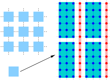
FIG. 1.: Visualization of the cluster perturbation approach for stripes: The infinite lattice is divided into unit cells. The unit cells differ for different stripe configurations. As shown here, the unit cell for a 3+1 configuration consists of two $3\times 6$ ladders on top of each other next to a 12-site chain. The 3-leg ladders on the left half of the unit-cell were diagonalized with a staggered magnetic field which was oriented in the opposite direction of the one on the right half. The hopping terms connecting the exactly–solved clusters ($3\times 6$ and $1\times 12$) as well as the hoppings connecting the unit cells are included via the cluster perturbation technique.

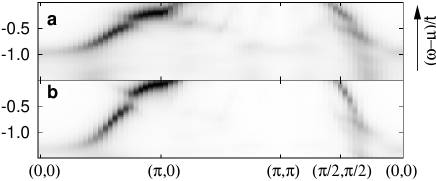
FIG. 2.: Single particle spectral function for a 2+2 bond-centered stripe configuration at 12% doping: Comparison of CPT calculations based on exact diagonalizations of two 2-leg $t$-$J$ ladders with $J=0.4t$ (a) and on exact diagonalizations of two 2-leg Hubbard ladders with $U=8t$ (b). The gray scale represents the weight of spectral function at the specific ($k,\omega$)-point with dark areas corresponding to high spectral weight.

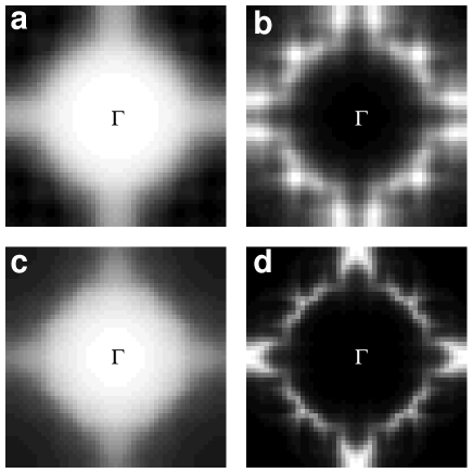
FIG. 3.: Integrated spectral weight of bond-centered stripe configurations at 12% doping; comparison of CPT calculations based on exact diagonalizations of $t$-$J$ ladders (a,b; $J=0.4t$) and Hubbard ladders (c,d; $U=8t$): (a,c) total integrated weight in photoemission ($n({\bf k})$), (b,d) low energy excitations (integrated weight in $E_{F}-0.2t<\omega<E_{F}$). The data are plotted for the whole Brillouin zone with the $\Gamma$-point in the center. The result of the stripe calculations have been symmetrized to account for the differently oriented stripe domains in real materials. Regions of high spectral weight correspond to white areas.

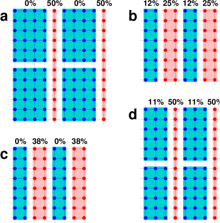
FIG. 4.: Unit cells for different stripe configurations: (a) 4+1 site-centered with 10 % doping; (b) 2+2 bond-centered with 19% doping ($2\times 8$ with 2 holes + $2\times 8$ with 4 holes); (c) 2+2 bond-centered with 19% doping ($2\times 8$ with 0 holes + $2\times 8$ with 6 holes); (d) 3+1 site-centered with 21 % doping.

FIG. 5.: Electron occupation in real space before (thick lines) and after (thin lines) application of CPT: (a,b,c,d) according to Fig.(4).

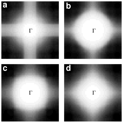
FIG. 6.: Total integrated spectral weight in photoemission $n(\vec{k})$: (a,b,c,d) according to Fig.(4).

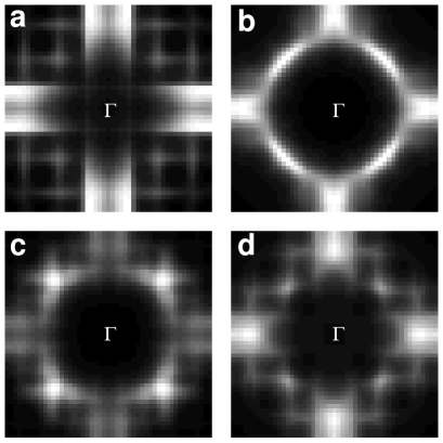
FIG. 7.: Integrated spectral weight around the Fermi surface: (a,b,c,d) according to Fig.(4).

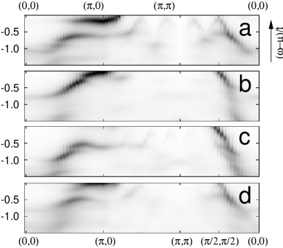
FIG. 8.: Density plot of the single particle spectral function: (a,b,c,d) according to Fig.(4).

REFERENCES

- [1] J.M. Tranquada et al., Nature 375, 561 (1995).
- [2] H.A. Mook et al., Nature 404, 729 (2000); Nature 395, 580 (1998).
- [3] B. Lake et al., Nature 400, 43 (1999).
- [4] Ph. Bourges, B. Keimer, L.P. Regnault, Y. Sidis,Proceedings of the MTSC2000 conference held in Klosters, cond-mat/0006085.
- [5] J. Zaanen and O. Gunnarsson, Phys. Rev. B 40, 7391 (1989).
- [6] M. Ichioka and K. Machida, J. Phys. Soc. Jpn. 68, 4020 (1999).
- [7] S.R. White, D.J. Scalapino,Phys. Rev. Lett. 80, 1272 (1998);Phys. Rev. Lett. 81, 3227 (1998);Phys. Rev. B 55, 6504 (1997).
- [8] M. Fleck, A. I. Lichtenstein, E. Pavarini, and A. M. Oles, Phys. Rev. Lett. 84, 4962 (2000).
- [9] B. Büchner, M. Breuer, A. Freimuth, and A. P. Kampf, Phys. Rev. Lett. 73, 1841 (1994).
- [10] D. Góra, K. Rościszewski, and A. M. Oleś, Phys. Rev. B 60, 7429 (1999).
- [11] S. A. Kivelson and V. J. Emery, Synthetic Metals 80, 151 (1996).
- [12] A.P. Harju, E. Arrigoni, W. Hanke, B. Brendel,S.A. Kivelson, cond-mat/0012293 (2000).
- [13] X.J. Zhou et al.,Science 286, 268 (1999).
- [14] X.J. Zhou et al.,cond-mat/0009002.
- [15] A. Ino et al.,Phys. Rev. B 62, 4137 (2000).
- [16] M. I. Salkola, V. J. Emery, and S. A. Kivelson, Phys. Rev. Lett. 77, 155 (1996).
- [17] M. G. Zacher, R. Eder, E. Arrigoni, and W. Hanke,Phys. Rev. Lett. 85, 2585 (2000).
- [18] V. J. Emery, S. A. Kivelson, and O. Zachar, Phys. Rev. B 56, 6120 (1997).
- [19] A. Ino et al.,J. Phys. Soc. Jpn. 68, 1496 (1999); cond-mat/0005473.
- [20] D. Sénéchal et al.,Phys. Rev. Lett. 84, 522 (2000).
- [21] P. Wróbel and R. Eder, Phys. Rev. B 62, 4048 (2000).
- [22] A. B. Harris and R. V. Lange, Phys. Rev. 157, 295 (1967).
- [23] See R. Eder, O. Rogojanu, and G. A. Sawatzky Phys. Rev. B 58, 7599 (98). For a similar derivation within the Hubbard-I approximation, see A. Dorneich et al, Phys. Rev. B 61, 12816 (2000).
- [24] S. Gopalan, T. M. Rice, and M. Sigrist, Phys. Rev. B 49, 8901 (1994).