*

Abstract

Simulation results of dense granular gases with particles of different size are compared with theoretical predictions concerning the pair-correlation functions, the collison rate, the energy dissipation, and the mixture pressure. The effective particle-particle correlation function, which enters the equation of state in the same way as the correlation function of monodisperse granular gases, depends only on the total volume fraction and on the dimensionless width ${\cal A}$ of the size-distribution function. The global equation of state is proposed, which unifies both the dilute and the dense regime.

The knowledge about a global equation of state is applied to steady-state situations of granular gases in the gravitational field, where averages over many snapshots are possible. The numerical results on the density profile agree perfectly with the predictions based on the global equation of state, for monodisperse situations. In the bi- or polydisperse cases, segregation occurs with the heavy particles at the bottom.

1 Introduction

The hard-sphere (HS) gas is a traditional, simple, tractable model for various phenomena and systems like e.g. disorder-order transitions, the glass transition, or simple gases and liquids [1, 2, 3]. A theory that describes the behavior of rigid particles is the kinetic theory [4, 1], where particles are assumed to be rigid and collisions take place in zero time (they are instantaneous), exactly like in the hard-sphere model. When dissipation is added to the HS model, one has the most simple version of a granular gas, i.e. the inelastic hard sphere (IHS) model. Granular media represent the more general class of dissipative, non-equilibrium, multi-particle systems [5]. Attempts to describe granular media by means of kinetic theory are usually restricted to certain limits like constant or small density [6] or weak dissipation [7, 8]. Also in the case of granular media, one has to apply higher order corrections to successfully describe the system under more general conditions [9, 10]. Already classical numerical studies showed that the equation of state can be expressed as some power series of the density in the low density regime [11, 2, 3], whereas, in the high density case, the free volume theory leads to useful results [12]. In the general situation, the granular system consists of particles with different sizes, a situation which is rarely addressed theoretically [13, 14, 15, 16]. However, the treatment of bi- and polydisperse mixtures is easily performed by means of numerical simulations [17, 18, 19].

In this study, theories and simulations for situations with particles of equal and different sizes are compared. In section 2 the model system is introduced and in 3 we review theoretical results and compare them with numerical results concerning correlations, collision rates, energy dissipation and pressure. Based on the numerical data, a global equation of state is proposed. This global equation of state is valid for arbitrary densities and mixtures with particles of different size, and it is used to explain the density profile in a dense system in the gravitational field in section 4. The results are summarized and discussed in section 5.

2 Model system

For the numerical modeling of the system, periodic, two-dimensional (2D) systems of volume $V=L_{x}L_{y}$ are used, with horizontal and vertical size $L_{x}$ and $L_{y}$, respectively. $N$ particles are located at positions ${\vec{r}}_{i}$ with velocities $\vec{v}_{i}$ and masses $m_{i}$. From any simulation, one can extract the kinetic energy $E=\frac{1}{2}\sum_{i=1}^{N}m_{i}\vec{v}_{i}^{2}$, dependent on time via the particle velocity $\vec{v}_{i}$. In 2D, the “granular temperature” is defined as $T=E/N$.

2.1 Polydispersity

The particles in the system have the radii $a_{i}$ randomly drawn from size distribution functions $w(a)$ as summarized in table 1 where the step-function $\theta[x]=1$ for $x\geq 1$ and $\theta[x]=0$ for $x<1$ is implied.

(i)	monodisperse	$w(a)=\delta(a-a_{0})$
(ii)	bidisperse	$w(a)=n_{1}\delta(a-a_{1})+n_{2}\delta(a-a_{2})$
(iii)	polydisperse	$w(a)=\frac{1}{2w_{0}a_{0}}\theta[a-(1-w_{0})a_{0}]\,\theta[(1+w_{0})a_{0}-a]~{}~{}$

Table 1: Size distribution functions used in this study.

The parameter $a_{0}$ is the mean particle radius $\langle a\rangle$ in cases (i) and (iii). In the bidisperse situation (ii), one has $a_{0}=\langle a\rangle=n_{1}a_{1}+n_{2}a_{2}=(n_{1}+(1-n_{1})/R)a_{1}$, with the fraction $n_{1}=N_{1}/(N_{1}+N_{2})$ of particles with size $a_{1}$ in a system with $N=N_{1}+N_{2}$ particles in total and $N_{2}$ particles with radius $a_{2}$. Thus, besides $n_{1}$, only the size ratio $R=a_{1}/a_{2}$ is needed to classify a bidisperse size distribution. The total volume fraction $\nu=\nu_{1}+\nu_{2}$ is the last relevant system parameter, since the partial volume fractions $\nu_{1,2}=N_{1,2}\pi a_{1,2}^{2}/V=n_{1,2}\nu a_{1,2}^{2}/\langle a^{2}\rangle$ can be expressed in terms of $n_{1}$ and $R$: Using the dimensionless moments

$$A_{k}=n_{1}+(1-n_{1})R^{-k}=\frac{\langle a^{k}\rangle}{a_{1}^{k}}~{},$$ (1)

one has $\nu_{1}=n_{1}\nu/A_{2}$ and $\nu_{2}=(1-n_{1})\nu/(R^{2}A_{2})$. Since needed later on, the expectation values for the moments of $a$ and their combination, the dimensionless width-correction ${\cal A}=\langle a\rangle^{2}/\langle a^{2}\rangle$, are summarized in table 2 in terms of $a_{1}$, $n_{1}$, and $R$ for the bidisperse situations and in terms of $a_{0}$ and $w_{0}$ in the polydisperse cases. Different values of $\nu$ are realized by shrinking or growing either the system or the particles.

		$\langle a\rangle$	$\langle a^{2}\rangle$	$\langle a\rangle^{2}/\langle a^{2}\rangle$
(i)	monodisperse	$a_{0}$	$a_{0}^{2}$	$1$
(ii)	bidisperse	$A_{1}a_{1}$	$A_{2}a_{1}^{2}$	${A_{1}^{2}}/{A_{2}}$
(iii)	polydisperse	$a_{0}$	$\left(1+{w_{0}^{2}}/{3}\right)a_{0}^{2}$	3 / $\left({3+w_{0}^{2}}\right)$

Table 2: Moments $\langle a\rangle$, $\langle a^{2}\rangle$ and ${\cal A}=\langle a\rangle^{2}/\langle a^{2}\rangle$ of the size distribution functions.

2.2 Particle Interactions

The particles are assumed to be perfectly rigid and to follow an undisturbed motion until a collision occurs as described below. Due to the rigidity, collisions occur instantaneously, so that an event driven simulation method [20, 21] can be used. Note that no multi-particle contacts can occur in this model. For a review on possible, more physical extensions of this model see Ref. [21].

A change in velocity – and thus a change in energy – can occur only at a collision. The standard interaction model for instantaneous collisions of particles with radii $a_{i}$, mass $m_{i}=(4/3)\pi\rho a_{i}^{3}$, and material density $\rho$ is used in the following. (Using the mass of a sphere is an arbitrary choice, however, using disks would not influence most of the results discussed below.) This model was introduced and also discussed for the more general case of rough particle surfaces in Refs. [7, 22, 23, 24, 25]. The post-collisional velocities $\vec{v}^{\prime}$ of two collision partners in their center of mass reference frame are given, in terms of the pre-collisional velocities $\vec{v}$, by

$$\vec{v}_{1,2}^{\prime}=\vec{v}_{1,2}\mp\frac{(1+r)~{}m_{12}}{m_{1,2}}\vec{v}_{n}~{},$$ (2)

with $\vec{v}_{n}\equiv\left[(\vec{v}_{1}-\vec{v}_{2})\cdot\hat{\vec{n}}\right]\hat{\vec{n}}$, the normal component of $\vec{v}_{1}-\vec{v}_{2}$ parallel to $\hat{\vec{n}}$, the unit vector pointing along the line connecting the centers of the colliding particles, and the reduced mass $m_{12}=m_{1}m_{2}/(m_{1}+m_{2})$. If two particles collide, their velocities are changed according to Eq. (2) and any $r(v_{n})$, dependent on $v_{n}=|\vec{v}_{n}|$, can be used. For a pair of particles, the change of the translational energy at a collision is $\Delta E=-m_{12}(1-r^{2})v_{n}^{2}/2$.

3 Simulation and theory

In the following, we compare simulations with different polydispersity, i.e. different size distribution functions $w(a)$, as summarized in table 3.

		$w(a)$ parameters	particles	${\cal A}$
A	monodisperse	$w_{0}=0$,	$N=1628$	1
B	monodisperse	$n_{1}=1$, $R=1$	$N=576$	1
C	bidisperse	$n_{1}=0.517$, $R=3/4$	$N=576$	0.9798
D1	bidisperse	$n_{1}=0.781$, $R=1/2$	$N=576$	0.8968
D2	bidisperse	$n_{1}=0.799$, $R=1/2$	$N=6561$	0.8998
E	polydisperse	$w_{0}=0.25$	$N=1425$	0.9796
F1	polydisperse	$w_{0}=0.5$	$N=1425$	0.9231
F2	polydisperse	$w_{0}=0.5$	$N=1521$	0.9231

Table 3: Simulation parameters for the simulations discussed below. Note that sets C and E have different $w(a)$ but almost identical values of ${\cal A}$.

3.1 Particle correlations

In monodisperse systems, the particle-particle pair correlation function at contact,

$$g_{2a}(\nu)=\frac{1-7\nu/16}{(1-\nu)^{2}}~{},$$ (3)

depends on the volume fraction only [1, 7, 3, 21, 8]. The particle-particle correlation function is obtained from the simulations by averaging over $M$ snapshots with $N$ particles, normalized to the value $g(r\gg 2a)=1$ for long distances in large systems, so that

$$g(r)=\frac{1}{M}\sum_{m=1}^{M}\frac{2V}{N(N-1)}\frac{1}{V_{r}}\sum_{i=1}^{N}\sum_{j=1}^{i-1}\theta[r_{ij}-r]\theta[r+\Delta r-r_{ij}]~{},$$ (4)

with $r_{ij}=|{\mathbf{r}}_{i}-{\mathbf{r}}_{j}|$, and where the two $\theta$ functions select all particle pairs $(i,j)$ with distance between $r$ and $r+\Delta r$. The weight $N(N-1)/2$ accounts for all pairs summed over, and the term $V_{r}=\pi(2r+\Delta r)\Delta r$ is the volume (area) of a ring with inner radius $r$ and width $\Delta r$. In Fig. 1, simulation results from set B (see table 3) with different $\nu$ are presented. Typical values used for the averages are e.g. $M=50$, and $\Delta r=a/10$. Besides fluctuations, the values at contact nicely agree with the theoretical predictions from Eq. (3), as indicated by the arrows – as long as the system is disordered (left panel in Fig. 1). In a more ordered system (right panel in Fig. 1), $g_{2a}(\nu)$ is not a good estimate. Instead, one obtains a long range order with peaks at $r/2a=1,\sqrt{3},2$, … , indicating the triangular lattice structure of the assembly.

Figure 1: Particle-particle correlation function $g(r)$ plotted against the normalized center-center distance $r/2a$. (Left) Disordered systems – the arrows indicate the values at contact from Eq. (3). (Right) Ordered systems with different axis scaling.

Figure 2: Particle-particle correlation function $g(r)$ plotted against the center-center distance normalized by the radius $a_{1}$ of the smaller particles, at a volume fraction of $\nu=0.60$. The arrows indicate the values $g_{11}$, $g_{12}$, and $g_{22}$ at contact. (Left) Bidisperse simulation from set C with $R=3/4$, and (Right) bidisperse simulation from set D1 with $R=1/2$.

For bidisperse situations, the pair correlation functions for equal species $g_{\rm 11}$ and $g_{\rm 22}$ are obtained by replacing $N$ in the first particle-sum in Eq. (4) by $N_{\rm 1}$ and $N_{\rm 2}$, respectively. For the correlation function $g_{\rm 12}$, it is necessary to perform the first particle-sum in Eq. (4) from $i=1$ to $N_{\rm 1}$, the second sum from $j=1$ to $N_{\rm 2}$, and to replace the weight $N(N-1)/2$ by $N_{\rm 1}N_{\rm 2}$ (in order to account for all pairs of different kind). In Fig. 2 simulation results from sets C and D1 for $\nu=0.6$ are compared to the analytical expressions Eqs. (90), (91), and (92) from Ref. [13], here expressed in terms of $A_{1,2}$, $R$, and $\nu$:

$$g_{\rm 11} = \frac{1-\nu\left(1-\frac{9}{16}\frac{A_{1}}{A_{2}}\right)}{(1-\nu)^{2}}~{},$$ (5)

$$g_{\rm 22} = \frac{1-\nu\left(1-\frac{9}{16R}\frac{A_{1}}{A_{2}}\right)}{(1-\nu)^{2}}~{},{\rm~{}~{}and}$$ (6)

$$g_{\rm 12} = \frac{1-\nu\left(1-\frac{9}{8(1+R)}\frac{A_{1}}{A_{2}}\right)}{(1-\nu)^{2}}~{}.$$ (7)

Note that all $g_{ij}$ are identical to $g_{2a}(\nu)$ in the monodisperse case with $R=1$ and $A_{1}=A_{2}=1$. The parameters used for averaging were $M=50$ and $\Delta r=a_{1}/118$ (Left) and $\Delta r=a_{1}/64$ (Right). A finer binning leads to stronger fluctuations, a rougher binning does not resolve the values at contact, however, within the statistical error, the agreement between theoretical predictions and numerical results is reasonable.

Figure 3: Particle-particle correlation function $g(r)$ plotted against the normalized center-center distance $r/2a_{0}$. (Left) Low density systems and (Right) high density systems with the same axis scaling.

Finally, in Fig. 3, particle correlation functions from polydisperse simulations (set F1) are presented. Due to the broad and continuous size distribution function, $g(r)$ is a smooth function with much less variety in magnitude than in the mono- and polydisperse situations discussed above. It more resembles the distribution function of a gas or liquid with a smooth interaction potential [3].

3.2 Collision rates and energy dissipation

In order to estimate the rate of change of energy in the system $\dot{T}=t_{E}^{-1}\Delta T$, the collision frequency $t_{E}^{-1}$ is needed. Rather than going into details concerning the calculation of $t_{E}^{-1}$, we will simply use the Enskog collision rate [2, 3, 21] for identical particles,

$$t_{E}^{-1}=\frac{4aN}{V}\sqrt{\pi}g_{2a}(\nu)\sqrt{T/m}~{},$$ (8)

and, equivalently, the inter-species collision rates

$$t_{ij}^{-1}=\frac{v^{\rm rel}_{ij}}{\lambda_{ij}}=\frac{2a_{ij}N_{j}}{V}\sqrt{\pi}g_{ij}\sqrt{T/(2m_{ij})}~{},$$ (9)

where all rates give the number of collisions of a particle per unit time, with $a_{ij}=a_{i}+a_{j}$. The temperature is here assumed to be independent of the particle species for the sake of simplicity. This is approximately true in the systems examined below, provided they stay rather homogeneous, but it is not true in general, since the cooling rates depend on the species.

In Eq. (9), the term $\sqrt{T/(m_{ij})}$ is proportional to the mean relative velocity $v^{\rm rel}_{ij}$ of a pair ($i$, $j$), so that the remainder $t_{ij}^{-1}/v^{\rm rel}_{ij}$ can be seen as a measure for the inverse interspecies mean free path $\lambda_{ij}$. The mean collision rate in the system is

$${\cal T}^{-1}_{\rm mix}=\sum_{i,j}n_{i}t_{ij}^{-1}=\frac{4a_{1}N}{V}\sqrt{\pi}\sqrt{T/m_{1}}\sum_{i,j}n_{i}n_{j}g_{ij}c_{ij}~{},$$ (10)

with $c_{11}=1$, $c_{12}=(1+R)/(2R)\sqrt{(1+R^{3})/2}$, and $c_{22}=\sqrt{R}$. Note that $c_{12}$ and $c_{22}$ depend on mass and density of the different species. The mean collision rate was tested for the monodisperse and bidisperse situations and showed the same quality of agreement as the pressure, which will be discussed in the next subsection. Therefore, we do not present data of the collision rates here, but perform a detailed numerical study of the mixture pressure below. However, we should remark that the interspecies collision rates are of the same order of magnitude, even if the species fluctuation velocities $v_{i}=\sqrt{T/m_{i}}$ strongly differ due to the differences in mass, also when the temperature $T=T_{i}=T_{j}=E/N$ is not species dependent. This means that the mean free distance between collisions compensates the speed; the distance traveled between collisions is proportional to the species velocity.

$\nu=0.30$ $\nu=0.60$
 
 
 
$\nu=0.70$ $\nu=0.85$
 
 

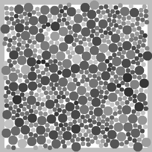
Figure 4: Snapshots from the bisdisperse simulations (set D1) for different volume fractions $\nu$. The grey-scale denotes the collision rate of the corresponding particle, the darkest particles had a collision rate of $1500$ s^-1, the lightest particles had a rate of less than $275$ s^-1. (These numbers have to be multiplied with $2/5$ for $\nu=0.30$ and with $4$ for $\nu=0.85$, in order to allow for a comparison of all pictures.)

In Fig. 4 several snapshots from simulation set D1 are presented. The grey-scale indicates the collision rates, dark particles collide more frequently than light particles, and the collision rate increases with the density, but as discussed above, the collision rates of the two species are comparable.

Knowing both the collision rates and the energy loss per collision

$$\Delta T_{ij}=-m_{ij}\frac{1-r^{2}}{2}(v^{\rm rel}_{ij})^{2}=-\frac{1-r^{2}}{2}T~{},$$ (11)

it is straightforward to compute the decay of energy as a function of time

$$\frac{dT}{dt}=\sum_{i,j}n_{i}t_{ij}^{-1}\Delta E_{ij}=-\frac{1-r^{2}}{2}{\cal T}_{\rm mix}^{-1}(t)T(t)~{},$$ (12)

where both $T(t)$ and ${\cal T}_{\rm mix}^{-1}(t)\propto\sqrt{T(t)}$ depend on time. The differential equation is easily solved and one gets the scaled temperature

$$\frac{T}{T_{0}}=\left(1+\frac{1-r^{2}}{4}{\cal T}_{\rm mix}^{-1}(0)\,t\right)^{-2}~{},$$ (13)

identical to the solution of the homogeneous cooling state of monodisperse disks [25], where $t_{E}^{-1}(0)$ is replaced by ${\cal T}_{\rm mix}^{-1}(0)$ from Eq. (10).

In Fig. 5, simulations from set D2 are presented for different values of $r<1$. The agreement between simulations and Eq. (13) is perfect for short times. With decreasing $r$, i.e. increasing dissipation, the deviations from the theory occur earlier due to the break-down of the homogeneity and the related simplifying assumptions of molecular chaos and Gaussian velocity distributions [26, 9].

Figure 5: Dimensionless temperature $T/T_{0}$ plotted against rescaled time $\tau={\cal T}_{\rm mix}^{-1}(0)t$ for different $r$, with double logarithmic axis. The symbols are simulation results from set D2, the solid lines correspond to Eq. (13). In the inset the quality factor $q_{T}=T_{\rm sim}/T_{\rm theory}$ is plotted against the time $\tau$.

3.3 Stress and the equation of state

The stress tensor, defined for a test-volume $V$, has two contributions, one from the collisions and the other from the translational motion of the particles. Using $a$ and $b$ as indices for the cartesian coordinates one has the components of the stress tensor (where the sign is convention)

$$\sigma^{ab}=\frac{1}{V}\left[\sum_{i}m_{i}v_{i}^{a}v_{i}^{b}-\frac{1}{\Delta t}\sum_{n}\sum_{j=1,2}\Delta p_{j}^{a}\ell_{j}^{b}\right]~{},$$ (14)

with $\ell_{j}^{b}$, the components of the vector from the center of mass of the two colliding particles $j$ to their contact points at collision $n$, where the momentum $\Delta p_{j}^{a}$ is exchanged. The sum in the left term runs over all particles $i$, the first sum in the right term runs over all collisions $n$ occuring in the time-interval $\Delta t$, and the second sum in the right term concerns the collision partners of collision $n$ – in any case the corresponding particles must be within the averaging volume $V$ [27, 28, 26, 21]. Note that the results may depend on the choice of $\Delta t$ and $V$ [29], however, a discussion of different averaging procedures and parameters is far from the scope of this study.

The mean pressure $p=(\sigma_{1}+\sigma_{2})/2~{}$, with the eigenvalues $\sigma_{1}$ and $\sigma_{2}$ of the stress tensor, can be obtained from simulations with rigid, elastic particles ($r=1$) and different volume fractions $\nu$ [21, 8]. The dimensionless reduced pressure from simulations agrees perfectly with the theoretical prediction [7]

$$P_{0}=PV/E-1=2\nu g_{2a}(\nu)~{},$$ (15)

with the total energy $E=(1/2)\Sigma_{i=1}^{N}m_{i}{\vec{v}}_{i}^{2}$. In Fig. 6 the simulation results for the dimensionless pressure $P=pV/E-1$ are compared to the kinetic theory result $P_{0}=2\nu g_{2a}(\nu)$ [21].

Figure 6: Dimensionless pressure $P=pV/E-1$ plotted against the volume fraction $\nu$ for different particle size-distribution functions. The bidisperse situation is identified by the size ratio $R$. The solid line corresponds to $P_{0}$. In the inset the quality factor $P/P_{0}$ is plotted for the same data. The wiggle of the $w_{0}=0$ data is discussed in more detail below.

When plotting $P$ against the volume fraction $\nu$ with a logarithmic vertical axis, the results for the different simulations can not be distinguished for $\nu<0.7$. In the monodisperse system, we obtain crystallization around $\nu=0.7$, and the data clearly deviate from $P_{0}$, i.e. the pressure is strongly reduced due to crystallization and, thus, enhanced free volume. The monodisperse data diverge at the maximum packing fraction $\nu^{\rm mono}_{\rm max}=\pi/(2\sqrt{3})$ in 2D. Note that one has to choose the system size such that a triangular lattice fits perfectly in the system, i.e. $L_{y}/L_{x}=\sqrt{3}h/2w$ with integer $h$ and $w$ – otherwise the maximum volume fraction is smaller. All other simulations are close to $P_{0}$ up to $\nu\approx 0.8$, where they begin to diverge; the bidisperse data with $R=1/2$, for example, diverge at $\nu^{\rm bi}_{\rm max}\approx 0.858$. The maximum packing fraction is smaller for the polydisperse size distributions used here and the crystallization, i.e. the pressure drop, does not occur for polydisperse packings with $w_{0}~{}_{\approx}^{>}~{}0.15$ (the data which lead to this approximate result are not shown). Since the logarithmic axis hides small deviations, we plot also the quality factor $P/P_{0}$ of the data in the inset. In this representation, values of unity mean perfect agreement, while smaller values correspond to an overestimation of the data by a factor of $P_{0}/P$ when $P_{0}$ would be used instead of the simulation results $P$. The deviations increase with increasing width of $w(a)$ and with increasing volume fraction. Note that there exists a deviation already for small $\nu$.

A more elaborate calculation in the style of Jenkins and Mancini, see Eq. (60) in [13], leads to the partial translational pressures $p^{t}_{i}=n_{i}E/V$ for species $i$ and to the collisional pressures $p^{c}_{ij}=\pi N_{i}N_{j}g_{ij}a_{ij}^{2}(1+r_{ij})T/(4V^{2})$ with the particle correlation functions from Eqs. (5)-(7) evaluated at contact, and $a_{ij}=a_{i}+a_{j}$. In the simulations from Fig. 6, the inter-species restitution coefficients are equal and elasticity is assumed, $r=r_{11}=r_{12}=r_{22}=1$. Note that the species temperatures are equal, so that the corresponding correction term can be dropped. Thus, the global pressure in the mixture is

$$p^{\rm m} = p^{t}_{1}+p^{t}_{2}+p^{c}_{11}+2p^{c}_{12}+p^{c}_{22}$$ (16)

$$= \frac{E}{V}\left[1+(1+r)\frac{\nu}{A_{2}a_{11}^{2}}(g_{11}a_{11}^{2}n_{1}^{2}+2g_{12}a_{12}^{2}n_{1}n_{2}+g_{22}a_{22}^{2}n_{2}^{2})\right]~{}$$ (17)

$$= \frac{E}{V}\left[1+{(1+r)\nu}g_{\cal A}(\nu)\right]~{}.$$ (18)

Assuming a monodisperse system as a test case, i.e.  inserting $R=A_{1}=A_{2}=1$, into Eq. (18), leads to the monodisperse solution $p^{\rm m}V/E-1=P_{0}$, as expected. The effective correlation function $g_{\cal A}(\nu)$ can be expressed in terms of the width-correction ${\cal A}$ of the size distribution so that

$$g_{\cal A}(\nu)=\frac{\left(1+{\cal A}\right)-\nu\left(1-{\cal A}/8\right)}{2(1-\nu)^{2}}~{},$$ (19)

with ${\cal A}={\langle a\rangle^{2}}/{\langle a^{2}\rangle}$. Note that ${\cal A}$ is well defined for any size distribution function, so that Eq. (19) can also be applied to polydisperse situations. In the limit of small volume fraction $\nu\rightarrow 0$, one can estimate the normalized pressure by

$$P_{1}=(1+r)\nu g_{2a}(\nu)\frac{1+{\cal A}}{2}~{},$$ (20)

as proposed by Zhang et al. [30], when disregarding the dependence of $g(r)$ on the types of the collision partners. The values of $P/P_{1}$ in the limit $\nu\rightarrow 0$ agree very well with the simulations. Using the effective particle correlations, one can define

$$P_{2}(\nu)=\frac{p^{\rm m}V}{E}-1=(1+r)\nu g_{\cal A}(\nu)~{},$$ (21)

and compare the resulting expected reduced pressure with the simulation results from Fig. 6. An almost perfect agreement between $P$ and $P_{2}(\nu)$ is obtained for $\nu<0.4$ and even for larger $\nu\approx 0.65$, the difference is always less than about two percent, and, the quality factors for all simulations collapse. Note that the quality is perfect (within less than 0.5 percent for all $\nu<0.65$) if $P_{2}(\nu)$ is multiplied by the empirical function $1-\nu^{4}/10$, as fitted to the quality factor $P/P_{2}$. Thus, based on our simulation results, we propose the corrected, nondimensional mixture pressure

$$P_{4}(\nu)=\frac{p^{\rm m}V}{E}-1=(1+r)\nu g_{\cal A}(\nu)\left[1-a_{g}\nu^{4}\right]~{},$$ (22)

with the empirical constant $a_{g}\approx 0.1$, for the pressure for all $\nu<0.65$. For larger $\nu$ the excluded volume effect becomes more and more important, leading to a divergence of $P/P_{4}$. Furthermore, in the high density regime, the behavior is strongly dependent on the width of the size distribution function, see Fig. 7.

       

Figure 7: Quality factor $P/P_{0}$ from the inset of Fig. 6. The lines give $P_{2}(\nu)/P_{0}$ from Eq. (21). In the inset, the simulation data for $P$ are rescaled by $P_{4}(\nu)$ from Eq. (22).

3.4 Accounting for the dense, ordered phase

The equation of state in the dense, ordered phase has been calculated by means of a free volume theory [31, 12, 32], that leads in 2D to the reduced pressure $P_{\rm fv}=1/(\sqrt{\nu_{\rm max}/\nu}-1)$ with the maximum volume fraction $\nu_{\rm max}$. Based on our simulation results we propse the corrected high density pressure

$$P_{\rm dense}=\frac{1}{\sqrt{\nu_{\rm max}/\nu}-1}\left[1+a_{d}(\nu_{\rm max}-\nu)^{a_{p}}\right]~{},$$ (23)

where the term in brackets $[\ldots]$ is a fit function with $a_{d}=0.340$ and $a_{p}=1.09$. The special case $a_{d}=0$ leads to the theoretical result $P_{\rm fv}$. In the left panel of Fig. 8, data from set B (see table 3) are presented, together with the “low” and “high” density predictions $P_{4}$ and $P_{\rm dense}$, respectively (dashed and dotted lines).

Figure 8: Dimensionless pressure $P$ from set B simulations (symbols) plotted against the volume fraction $\nu$. (Left) The dashed lines are $P_{4}$ from Eq. (22) and $P_{\rm dense}$ from Eq. (23). The thick solid line is $Q$, the corrected global equation of state from Eq. (24) with the fit-parameters $a_{g}=0.1$, $a_{d}=0.340$, $a_{p}=1.09$, $\nu_{c}=0.701$, $\nu_{\rm max}=0.9069$, and $m_{0}=0.00928$. The thin solid line is $Q_{0}$ without corrections, i.e.  $a_{g}=0$, $a_{d}=0$, and $m_{0}=0.0015$ and $\nu_{c}=0.7$, so that $Q_{0}=P_{2}+m(\nu)[P_{\rm fv}-P_{2}]$. (Right) Analogous data from set D1, where only $\nu_{\rm max}=0.858$ is different from the left panel.

To our knowledge, no theory exists, which combines the disordered and the ordered regime. Therefore, we propose a global equation of state

$$Q=P_{4}+m(\nu)[P_{\rm dense}-P_{4}]~{},$$ (24)

with an empirical merging function

$$m(\nu)=\frac{1}{1+\exp\left(-(\nu-\nu_{c})/m_{0}\right)}~{}$$ (25)

which selects $P_{4}$ for $\nu\ll\nu_{c}$ and $P_{\rm dense}$ for $\nu\gg\nu_{c}$ with the width of the transition $m_{0}$. In Fig. 8, the fit parameters $\nu_{c}\approx 0.70$ and $m_{0}\approx 0.009$ lead to qualitative and quantitative agreement between $Q$ (thick line) and the simulation results (symbols). However, also a simpler version $Q_{0}$ (thin line) without numerical corrections leads to reasonable agreement when $m_{0}=0.015$ is used, except for the transition region. The pressure drop when $\nu$ is increased above $\nu_{c}$ is qualitatively reproduced but no negative slope occurs. Due to the latter fact, the expression $Q_{0}$ allows for an easy numerical integration of $P$. We selected the parameters for $Q_{0}$ as a compromise between the quality of the fit on the one hand and the treatability of the function on the other hand.

Remarkably, as one can see from Fig. 8 (Right), the dimensionless pressure $Q$ from Eq. (24) describes, at least qualitatively, the behavior of the polydisperse simulations when $\nu_{\rm max}=0.858$ is used. Note that the pressure drop at the transition $\nu_{c}\approx 0.7$ from the low density, disordered regime to the high density, ordered regime, is almost non-existent, since $P_{4}$ and $P_{\rm dense}$ are almost collapsing in this range of density.

4 Pressure gradient due to gravity

In an experiment on earth, usually gravity plays an important role, it introduces a pressure gradient. Therefore, the density and pressure profiles of granular systems in equilibrium in the gravitational field are examined in the following. Here, a horizontal wall at $z=0$ is introduced in a periodic two dimensional system of width $L=l_{x}/(2a)$, infinite height, and the gravitational acceleration $g=1$ ms^-2.

4.1 Density profile in dilute systems

In the special case of low density, one can use the equation of state of an ideal gas and express the pressure as a function of the energy density:

$$p=\frac{E}{V}=nT~{},$$ (26)

with the number density $n=N/V=n(z)=\nu(z)/(\pi a^{2})$ and the “granular temperature” $T=E/N$ in two dimensions.

The gradient of pressure ${dp}/{dz}$ compensates for the weight $nmgLdz$ of the particles in a layer of height $dz$, so that

$$\frac{dp}{dz}=\frac{dp}{d\nu}\frac{d\nu}{dz}=-nmg$$ (27)

Separation of variables and the assumption of a constant temperature leads to the density profile for an ideal gas

$$\nu(z)=\nu_{0}\exp\left(-\frac{mg(z-z_{0})}{T}\right){\rm~{}~{}~{}or~{}~{}~{}}z(\nu)=z_{0}+{z_{T}}\ln\frac{\nu_{0}}{\nu}~{},$$ (28)

with $\nu<\nu_{0}$ and $z_{T}=T/(mg)$. In a system with a constant particle number $N$, one has

$$N\stackrel{{\scriptstyle!}}{{=}}\frac{L}{\pi a^{2}}\int_{z_{0}}^{\infty}\nu(z)dz=\frac{L}{\pi a^{2}}\int_{0}^{\nu_{0}}\left(z(\nu)-z_{0}\right)d\nu~{}.$$ (29)

Eq. (29) allows to determine analytically the volume fraction $\nu_{d}$ at the bottom $z_{0}$, in the dilute limit, by integration of $z(\nu)$

$$\nu_{d}=\frac{N\pi a^{2}mg}{TL}=\frac{N\pi a^{2}}{z_{T}L}~{},$$ (30)

defined here for later use.

This case can be extended to dilute and weakly dissipative systems, since the temperature is almost constant except for the bottom boundary layer [8, 33]. In the following we rather extend it to arbitrary density, but keep $r=1$.

4.2 Density profile for a monodisperse hard sphere gas

In the dense case, Eq. (26) is modified to

$$p=nT\left[1+2\nu g_{2a}(\nu)\right]~{},$$ (31)

using Eq. (15) with $r=1$, and inserting Eq. (31) into Eq. (27) leads to

$$\pi a^{2}\frac{dp}{dz}=\frac{d}{d\nu}\left[\nu T(1+2\nu g_{2a}(\nu))\right]\frac{d\nu}{dz}=-\nu mg~{}.$$ (32)

Assuming again that $T$ is constant, one gets

$$\frac{d}{d\nu}[\ldots]=T\,\left\{1+\frac{\partial}{\partial\nu}\left(2\nu^{2}g_{2a}(\nu)\right)\right\}=T\,\frac{8+8\nu+3\nu^{2}-\nu^{3}}{8(1-\nu)^{3}}~{},$$ (33)

which, inserted in Eq. (32), allows integration from $\nu_{0}$ to $\nu$ and from $z_{0}$ to $z$:

$$\int^{\nu}_{\nu_{0}}\left\{\frac{8}{\nu^{\prime}}+\frac{7}{1-\nu^{\prime}}+\frac{7}{(1-\nu^{\prime})^{2}}+\frac{18}{(1-\nu^{\prime})^{3}}\right\}d\nu^{\prime}=-\frac{8mg}{T}\int_{z_{0}}^{z}dz^{\prime}~{},$$ (34)

and leads to an implicit definition of $\nu(z)$:

$$\left[\ln\nu^{\prime}-\frac{7}{8}\ln(1-\nu^{\prime})+2g_{2a}(\nu^{\prime})\right]_{\nu_{0}}^{\nu(z)}=-\frac{z-z_{0}}{z_{T}}~{}.$$ (35)

We express $z$ as a function of the volume fraction

$$\frac{z(\nu)-z_{0}}{z_{T}}=\ln\frac{\nu_{0}}{\nu}-\frac{7}{8}\ln\frac{1-\nu_{0}}{1-\nu}+2g_{2a}(\nu_{0})-2g_{2a}(\nu)~{},$$ (36)

with the unknown volume fraction $\nu_{0}$ at $z_{0}$, which, however, is determined using Eq. (29):

$$\frac{N_{0}\pi a^{2}}{z_{T}L}=\nu_{d}\stackrel{{\scriptstyle!}}{{=}}\int_{0}^{\nu_{0}}\frac{z(\nu)-z_{0}}{z_{T}}d\nu={\nu_{0}}\,\frac{8+\nu_{0}^{2}}{8(1-\nu_{0})^{2}}~{},$$ (37)

where $N_{0}$ is the number of particles above a given height $z_{0}$. Only if $z_{0}=0$, one has $N_{0}=N$. This leads to a third order polynomial for $\nu_{0}$,

$$\nu_{0}^{3}-8\nu_{d}\nu_{0}^{2}+(16\nu_{d}+8)\nu_{0}-8\nu_{d}=0~{},$$ (38)

which can be solved analytically [34], and always has at least one real solution. Note that the function $g_{2a}(\nu)$ is wrong at high densities $\nu>\nu_{c}$, so that also the pressure is not correct for high densities. This fact is discussed also by D. Hong [35], who performed the three dimensional calculations analogous to our 2D calculus in this section.

4.3 Comparison with simulations

In this subsection, the theoretical density profile in Eq. (36), with the parameter $\nu_{0}$ determined via Eq. (38), is compared to numerical simulations with the parameters as specified in table 4. In Fig. 9, the rescaled height $z/z_{T}$ is plotted against the volume fraction $\nu$, according to Eq. (36). Note that even when the simulation parameters are rather arbitrary, the data follow a master-curve from $\nu=0$ to $\nu=\nu_{0}$ (or equivalently from $z=\infty$ to $z=0$) only shifted vertically such that $z(\nu_{0})=0$. The agreement between simulation and theory is almost perfect, except for simulation IV where densities above $\nu\approx 0.65$ are observed, i.e. above the limit of validity of the equation of state. Therefore, the numerical values of $z/z_{T}$ are systematically smaller than the theoretical line obtained for $\nu_{0}$ from table 4.

	$N$	$L/(2a)$	$T$ (kg m2 s-2)	$z_{T}/(2a)$	$\nu_{d}$	$\nu_{0}$
I	1562	100	$3.07\times 10^{-8}$	29.4	0.418	0.240
II	3000	100	$2.22\times 10^{-8}$	21.2	1.110	0.396
III	1000	100	$2.61\times 10^{-9}$	2.49	3.151	0.567
IV	1000	10	$6.13\times 10^{-9}$	5.85	13.41	0.755

Table 4: Simulation parameters for density profile measurements. In these simulations, the particle radius $a=5\times 10^{-4}$ m and the particle mass $m=1.047\times 10^{-6}$ kg were not changed.

The only way to get the correct theoretical density profile is for points with $\nu<0.65$. The value of $z_{0}=13.5z_{T}$, where $\nu(z_{0}/z_{T})=0.65$, is taken from the simulation data and the normalization accounts only for the $N_{0}$ particles above $z_{0}$. The resulting density profile (dashed line) nicely agrees with the simulations, and its limit of validity is inidcated by the angle at $z/z_{T}=13.5$ and $\nu=0.65$.

Figure 9: Rescaled height $z/z_{T}$ plotted against the volume fraction $\nu$ from four different simulations, see table 4, with logarithmic horizontal axis. Symbols are simulation data and the lines correspond to Eq. (36) with the respective value of $\nu_{0}$.

The reason for the increased density at low $z/z_{T}$ in the case of simulation IV is the pressure drop due to crystallization in the equation of state, see Fig. 7. A higher density is necessary to sustain a given pressure when $\nu>0.65$. The data for the lowest $z/z_{T}\approx 0$ are slightly off due to the wall induced ordering at $z/z_{T}=0$.

If, instead of $2\nu g_{2a}(\nu)$ in Eq. (32), we use the more general form $Q_{0}$, we have to integrate the differential equation $dp/dz=\nu mg/(\pi a^{2})$ numerically with $p=nT(1+Q_{0})$ and the condition that Eq. (29) is fulfilled. Simulation IV and the numerical solution are compared in Fig. 10. The qualitative behavior of the density profile is well reproduced by the numerical solution with $\nu(z_{0}=0)=0.8016$. Note that the averaging result is dependent on the binning – we evidence strong coarse-graining effects in the dense, ordered region with densities $\nu>0.70$.  
 
 

Figure 10: Rescaled height $z/z_{T}$ plotted against the volume fraction $\nu$ from simulation IV, see table 4. The symbols are simulation data of the particle-center with a rough binning $\Delta z=0.01007$ m. The solid line is the density from the same data but with a much finer binning $\Delta z=0.00184$ m. Both binnings start at $z_{0}+\frac{1}{5}a$ with $z_{0}=0$. The dashed line corresponds to the numerical solution of Eq. (32) with $p=nT(1+Q_{0})$. The transition density $\nu_{c}\approx 0.7$ is indicated by an arrow.

Figure 11: Dimensionless height $z/(2a_{1})$ plotted against the volume fraction (in logarithmic scale). The thick, dashed line gives $1-{\cal A}$ (which is zero when only the small species is present at large heights), while the solid line indicates the total volume fraction of the mixture $\nu^{\rm m}=\nu_{1}+\nu_{2}$.

4.4 Bidisperse systems with gravitation

In Fig. 11 the species volume fractions $\nu_{1}$ and $\nu_{2}$ are plotted against the vertical coordinate $z/(2a_{1})$. The data are obtained after long equilibration, in a system with $N=2000$ particles, width $L_{x}=l_{x}/(2a_{1})=100$, and the size distribution of set D1 in the previous section, with $a_{1}=0.0005$ m. The particles are no longer mixed, as in the homogeneous, periodic systems of the previous section. Segregation takes place, the larger and heavier particles (squares) settle close to the bottom, whereas the gas of small and lighter particles (circles) extends to larger heights. Knowing both volume fractions, one could compute ${\cal A}$ as a function of the height, and insert it into Eq. (19) in order to compute the density profile.

5 Summary and Outlook

In summary, we reviewed existing theories for dilute and dense almost elastic, smooth, 2D granular gases. For mono-, bi-, and polydisperse systems, we compared theoretical predictions with numerical simulations of various systems. The collision frequency, the energy dissipation and the equation of state, i.e. the scaled pressure, are nicely predicted by the theoretical expressions up to intermediate densities. Especially, for arbitrary particle size distribution functions, the equation of state can be written in a nice form which only contains the width-correction ${\cal A}$ of the size-distribution function. A small, empirical correction can be added to the theories to raise the quality even further. Finally, a merging function that connects the low and high density theories is proposed to give a global equation of state for all densities and size distribution functions.

The equation of state is used to compute analytically and numerically the density profile of an elastic, monodisperse granular gas in the gravitational field. When a mixture is simulated, segregation is observed, a case to which the theory cannot be applied. For densities below $\nu\approx 0.65$, the analytical solution works well, for higher densities close to the maximum density, one has to use a numerical solver, since the global equation of state cannot be integrated analytically. The strange shape of the density profile, as obtained from simulations, is nicely reproduced.

The simulations and the theories presented here were applied to homogeneous systems. The range of applicability may be reduced by the fact that already weak dissipation can lead to strong inhomogeneities in density, temperature, and pressure. In a freely cooling system, for example, clustering leads to all densities between $\nu\approx 0$ and $\nu\approx\nu_{\rm max}$. The proposed global equation of state is a necessary tool to account for such strong inhomogeneities with very high densities, above which the low-density theory fails. For another approach to handle the high density regions, see Ref. [35].

The proposed global equation of state is based on a limited amount of data. It has to be checked, whether it still makes sense in the extreme cases of narrow $w(a)$, where crystallization effects are rather strong, and for extremely broad, possibly algebraic $w(a)$, where ${\cal A}$ is not defined. What also remains to be done is to find similar expressions not only for pressure and energy dissipation rate but also for viscosity and heat-conductivity and to extend the theory to three dimensions

References

- [1] S. Chapman and T. G. Cowling. The mathematical theory of nonuniform gases. Cambridge University Press, London (1960).
- [2] J. M. Ziman. Models of Disorder. Cambridge University Press, Cambridge (1979).
- [3] J. P. Hansen and I. R. McDonald. Theory of simple liquids. Academic Press Limited, London (1986).
- [4] L. D. Landau and E. M. Lifschitz. Physikalische Kinetik. Akademie Verlag Berlin, Berlin (1986).
- [5] H. J. Herrmann, J.-P. Hovi, and S. Luding, editors. Physics of dry granular media - NATO ASI Series E 350. Kluwer Academic Publishers, Dordrecht 1998.
- [6] P. K. Haff. Grain flow as a fluid-mechanical phenomenon. J. Fluid Mech. 134, 401 (1983).
- [7] J. T. Jenkins and M. W. Richman. Kinetic theory for plane flows of a dense gas of identical, rough, inelastic, circular disks. Phys. of Fluids 28, 3485 (1985).
- [8] P. Sunthar and V. Kumaran. Temperature scaling in a dense vibrofluidized granular material. Phys. Rev. E 60, 1951 (1999).
- [9] T. P. C. van Noije and M. H. Ernst. Velocity distributions in homogeneously cooling and heated granular fluids. Granular Matter 1, 57 (1998).
- [10] N. Sela and I. Goldhirsch. Hydrodynamic equations for rapid flows of smooth inelastic spheres, to burnett order. J. Fluid Mech. 361, 41 (1998).
- [11] B. J. Alder and T. E. Wainwright. Studies in molecular dynamics. I. General method. J. Chem. Phys. 31, 459 (1959).
- [12] R. J. Buehler, Jr. R. H. Wentorf, J. O. Hirschfelder, and C. F. Curtiss. The free volume for rigid sphere molecules. J. of Chem. Phys. 19, 61 (1951).
- [13] J. T. Jenkins and F. Mancini. Balance laws and constitutive relations for plane flows of a dense, binary mixture of smooth, nearly elastic, circular discs. J. Appl. Mech. 54, 27 (1987).
- [14] B. Arnarson and J. T. Willits. Thermal diffusion in binary mixtures of smooth, nearly elastic spheres with and without gravity. Phys. Fluids 10, 1324 (1998).
- [15] B. Arnarson. Simplified kinetic theory of a binary mixture of nearly elastic, smooth disks, preprint (1999).
- [16] J. T. Willits and B. Arnarson. Kinetic theory of a binary mixture of nearly elastic disks, preprint (1999).
- [17] E. Dickinson. Molecular dynamics simulation of hard-disc mixtures. The equation of state. Molecular Physics 33, 1463 (1977).
- [18] S. Luding, O. Strauß, and S. McNamara. Segregation of polydisperse granular media in the presence of a temperature gradient. In T. Rosato, editor, IUTAM Symposium on Segregation in Granular Flows, Kluwer Academic Publishers (2000).
- [19] S. McNamara and S. Luding. A simple method to mix granular materials. In T. Rosato, editor, IUTAM Symposium on Segregation in Granular Flows, Kluwer Academic Publishers (2000).
- [20] B. D. Lubachevsky. How to simulate billards and similar systems. J. of Comp. Phys. 94, 255 (1991).
- [21] S. Luding and S. McNamara. How to handle the inelastic collapse of a dissipative hard-sphere gas with the TC model. Granular Matter 1, 113 (1998). cond-mat/9810009.
- [22] O. R. Walton and R. L Braun. Stress calculations for assemblies of inelastic spheres in uniform shear. Acta Mechanica 63, 73 (1986).
- [23] C. K. K. Lun. Kinetic theory for granular flow of dense, slightly inelastic, slightly rough spheres. J. Fluid Mech. 233, 539 (1991).
- [24] A. Goldshtein and M. Shapiro. Mechanics of collisional motion of granular materials. Part 1. General hydrodynamic equations. J. Fluid Mech. 282, 75 (1995).
- [25] S. Luding, M. Huthmann, S. McNamara, and A. Zippelius. Homogeneous cooling of rough dissipative particles: Theory and simulations. Phys. Rev. E 58, 3416 (1998).
- [26] S. Luding. Clustering instabilities, arching, and anomalous interaction probabilities as examples for cooperative phenomena in dry granular media. T.A.S.K. Quarterly, Scientific Bulletin of Academic Computer Centre of the Technical University of Gdansk 2, 417 (July 1998).
- [27] J. D. Goddard. Microstructural origins of continuum stress fields - a brief history and some unresolved issues. In D. DeKee and P. N. Kaloni, editors, Recent Developments in Structered Continua. Pitman Research Notes in Mathematics No. 143, p. 179, New York, Longman, J. Wiley (1986).
- [28] F. Emeriault and C. S. Chang. Interparticle forces and displacements in granular materials. Computers and Geotechnics 20, 223 (1997).
- [29] I. Goldhirsch. Kinetics and dynamics of rapid granular flows. In H. J. Herrmann, J.-P. Hovi, and S. Luding, editors, Physics of dry granular media - NATO ASI Series, p. 371, Dordrecht, Kluwer Academic Publishers (1998).
- [30] J. Zhang, R. Blaak, E. Trizac, J. A. Cuesta, and D. Frenkel. Optimal packing of polydisperse hard-sphere fluids. preprint (1999).
- [31] J. G. Kirkwood, E. K. Maun, and B. J. Alder. Radial distribution functions and the equation of state of a fluid composed of rigid spherical molecules. J. Chem. Phys. 18, 1040 (1950).
- [32] W. W. Wood. Note on the free volume equation of state for hard spheres. J. Chem. Phys. 20, 1334 (1952). Letters to the Editor.
- [33] J. Eggers. Sand as Maxwell’s demon. Phys. Rev. Lett. 83, 5322 (1999).
- [34] I. N. Bronstein and K. A. Semendjajew. Taschenbuch der Mathematik. Teubner, Leipzig (1979).
- [35] D. C. Hong. Fermi Statistics and Condensation, (in this volume).