Dynamics of a mesoscopic qubit under continuous quantum measurement
Abstract
We present the conditional quantum dynamics of an electron tunneling between two quantum dots subject to a measurement using a low transparency point contact or tunnel junction. The double dot system forms a single qubit and the measurement corresponds to a continuous in time readout of the occupancy of the quantum dot. We illustrate the difference between conditional and unconditional dynamics of the qubit. The conditional dynamics is discussed in two regimes depending on the rate of tunneling through the point contact: quantum jumps, in which individual electron tunneling current events can be distinguished, and a diffusive dynamics in which individual events are ignored, and the time-averaged current is considered as a continuous diffusive variable. We include the effect of inefficient measurement and the influence of the relative phase between the two tunneling amplitudes of the double dot/point contact system.
pacs:
73.63.Kv,83.35.Be,03.65.Ta,03.67.LxI Introduction
In condensed matter physics, measurements are usually made on many identical quantum systems prepared at the same time. For example, in nuclear or electron magnetic resonance experiments, an ensemble of systems of nuclei and electrons are probed to obtain the resonance signals. In this case, the measurement result is an average response of the ensemble. On the other hand, various proposed condensed-matter quantum computer architectures [2, 3, 4, 5] demand the need to readout physical properties of a single electronic qubit, such as charge or spin at a single electron level. This is a non-trivial problem since it involves an individual quantum particle measured by a practical detector in a realistic environment. It is particularly important to take account of the decoherence introduced by the measurements on the qubit as well as to understand how the quantum state of the qubit, conditioned on a particular single realization of measurement, evolves in time for the purpose of quantum computing.
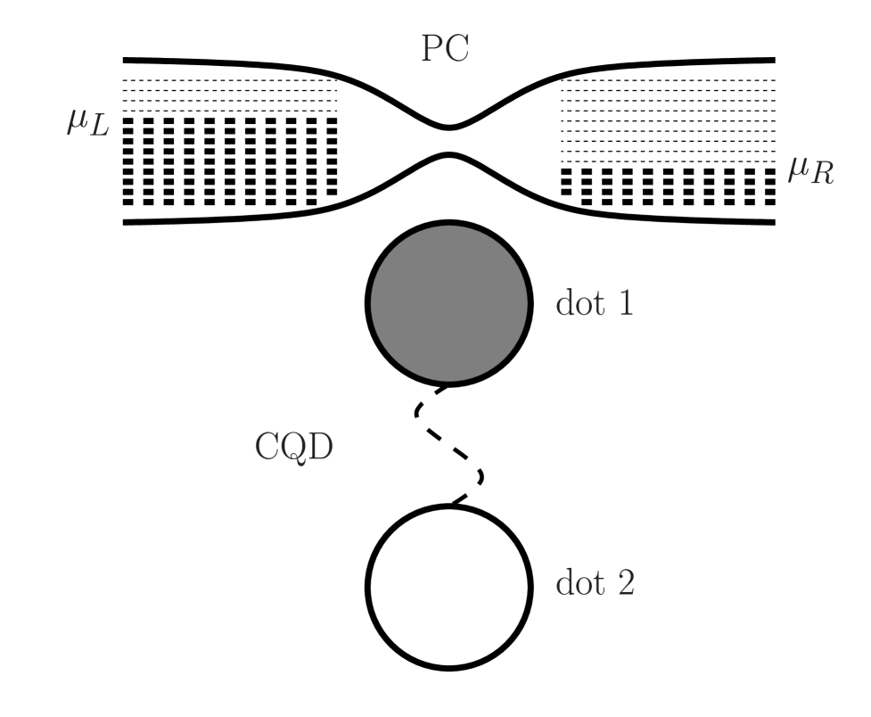
We consider, in this paper, the problem of an electron tunneling between two coupled quantum dots (CQD’s), a two-state quantum system (qubit), using a low-transparency point contact (PC) or tunnel junction as a detector (environment) continuously measuring the position of the electron, schematically illustrated in Fig. 1. This problem has been extensively studied in Refs. [6, 7, 8, 9, 10, 11, 12, 13, 14, 15]. The case of measurements by a general quantum point contact detector with arbitrary transparency has also been investigated in Refs. [16, 17, 18, 19, 20, 21]. In addition, a similar system measured by a single electron transistor rather than a PC has been studied in Refs. [22, 11, 9, 12, 14, 23, 24]. The influence of the detector (environment) on the measured system can be determined by the reduced density matrix obtained by tracing out the environmental degrees of the freedom in the total, system plus environment, density matrix. The master equation (or rate equations for the reduced-density-matrix elements) for the CQD system (qubit) has been derived and analyzed in Refs. [6, 15]. However, this (unconditional) master equation describes only the ensemble average property for the CQD system. Integrating or tracing out the PC environmental degrees of the freedom is equivalent to completely ignoring or averaging over the results of all measurement records (electron current records in this case). In this sense, the PC is treated as a pure environment rather than a measurement device which can provide information about the change of the state of the qubit. On the other hand, if a measurement is made on the system and the results are available, the state or density matrix is a conditional state conditioned on the measurement results. Hence the deterministic, unconditional master equation cannot describe the conditional dynamics of the qubit in a single realization of continuous measurements which reflects the stochastic nature of an electron tunneling through the PC barrier.
Korotkov [8, 10, 14] has obtained the Langevin rate equations for the CQD system measured by a ideal PC detector. These rate equations describe the random evolution of the density matrix that both conditions, and is conditioned by, the PC detector output. Recently, we [15] presented a quantum trajectory [25, 26, 27, 28, 29, 30, 31, 32, 33, 34, 35] measurement analysis of the same system. We found that the conditional dynamics of the CQD system can be described by the stochastic Schrödinger equation for the conditioned state vector, provided that the information carried away from the CQD system by the PC reservoirs can be recovered by the perfect detection of the measurements. We also analyzed the localization rates at which the qubit becomes localized in one of the two states when the coupling frequency between the states is zero. We showed that the localization time discussed there is slightly different from the measurement time defined in Refs. [22, 11, 12]. The mixing rate at which the two possible states of the qubit become mixed when was calculated as well and found in agreement with the result in Ref. [11, 12]. In this paper, we focus on the qubit dynamics conditioned on a particular realization of the actual measured current through the PC device. Especially, we take into account the effect of inefficient measurement on the conditional dynamics and illustrate the conditional quantum evolutions by numerical simulations.
The problem for a “non-ideal” detector was discussed in Refs. [8, 9, 10]. There the non-ideality of the detector is modeled as two ideal detectors “in parallel” with inaccessible output of the second detector. The information loss is due to the interaction with the second detector, treated as a “pure environment”, (which does not affect the detector current). As a consequence, the decoherence rate, , in that case is larger than the decoherence rate for the PC as an environment alone, . Hence an extra decoherence term, , for example, is added in the rate equation . However, this approach does not account for the inefficiency in the measurements, which arises when the detector sometimes misses detection. In that case, there is still only one PC detector (environment) and disregarding all measurement records leads to . Furthermore, the detector current is affected and in fact reduced by the inefficiency in the measurements.
In this paper, we analyze the conditional qubit dynamics analytically and numerically. We take into account the effect of inefficient measurement of the PC detector on the dynamics of the qubit. The different behavior of unconditional and conditional evolution is demonstrated. We present the conditional quantum dynamics over the full range of behavior, from quantum jumps to quantum diffusion. [15] In Refs. [6, 8, 10, 14], the two tunneling amplitudes of the CQD-PC model were assumed to be real. In Ref. [15], the relative phase between them was taken into account. Here, we discuss and illustrate furthermore their influence on the qubit dynamics. In Sec. II, we describe the model Hamiltonian and the unconditional master equation. We then obtain in Sec. III the quantum-jump and quantum-diffusive, conditional master equations for the case of inefficient measurements. Sec. IV is devoted to the analysis for the qubit dynamics. Numerical simulations of the conditional evolution are presented in this section. Finally, a short conclusion is given in Sec. V. In the Appendix, the stationary noise power spectrum of the current fluctuations through the PC barrier is calculated in terms of the quantum-jump formalism.
II Unconditional master equation for the CQD and PC model
The appropriate way to approach quantum measurement problems may be to treat the measured system, the detector (environment), and the coupling between them together microscopically. Following from Refs. [6, 8, 10], We describe the whole system (see Fig. 1) by the following Hamiltonian:
| (1) |
where
| (2) | |||||
| (3) | |||||
| (4) |
represents the effective tunneling Hamiltonian for the measured CQD system (mesoscopic qubit). For simplicity, we assume strong inner and inter dot Coulomb repulsion, so only one electron can occupy this CQD system. We label each dot with an index (see Fig. 1) and let () and represent the electron annihilation (creation) operator and energy for a single electron state in each dot respectively. The coupling between these two dots is given by . The tunneling Hamiltonian for the PC detector is represented by where , and , are respectively the fermion (electron) field annihilation operators and energies for the left and right reservoir states at wave number . One should not be confused by the electron in the CQD with the electrons in the PC reservoirs. The tunneling matrix element between states and in left and right reservoir respectively is given by . Eq. (4), , describes the interaction between the detector and the measured system, depending on which dot is occupied. When the electron in the CQD system is near the PC (i.e., dot is occupied), there is a change in the PC tunneling barrier. This barrier change results in a change of the effective tunneling amplitude from . As a consequence, the current through the PC is also modified. This changed current can be detected, and thus a measurement of the location of the electron in the CQD system is effected.
The (unconditional) master equation of the reduced density matrix for the CQD system (qubit) has been obtained in Refs. [6, 15]. Under similar assumptions and approximations as in Ref. [15], the zero-temperature, [36] Markovian master equation of the qubit can be written as:
| (6) | |||||
| (7) |
where is the occupation number operator for dot 1 and the parameters and are given by
| (9) | |||||
| (10) |
where and are the average electron tunneling rates through the PC barrier without and with the presence of the electron in dot 1 respectively. In Eq. (II), is the external bias applied across the PC (where is the electronic charge, and and stand for the chemical potentials in the left and right reservoirs respectively), and are energy-independent tunneling amplitudes near the average chemical potential, and and are the energy-independent density of states for the left and right reservoirs. In Eq. (6), the superoperator [28, 37, 31] is defined as:
| (11) |
where
| (12) | |||||
| (13) |
Finally, Eq. (7) defines the Liouvillian operator . The form of the master equation (6), defined through the superoperator , preserves the positivity of the density matrix operator . Such a Markovian master equation is called a Lindblad [38] form.
Evaluating the density matrix operator in the same basis as in Ref. [6], we obtain
| (15) | |||||
| (16) |
where is the energy mismatch between the two dots, , and and are the probabilities of finding the electron in dot 1 and dot 2 respectively. The corresponding logical qubit states are then and . The rate equations for the other two density matrix elements can be easily obtained from the relations: and . Compared to an isolated CQD system, the presence of the PC detector (environment) introduces two effects to the CQD system. First, the imaginary part of (the last term in Eq. (16)) causes an effective shift in the energy mismatch between the two dots. Second, it generates a decoherence (dephasing) rate
| (17) |
for the off-diagonal density matrix elements. The relative phase between the two complex tunneling amplitudes may produce additional effects on conditional dynamics of the CQD system as well. This will be shown later when we discuss conditional dynamics. Physically, the presence of the electron in dot 1 (state ) raises the effective tunneling barrier of the PC due to electrostatic repulsion. As a consequence, the effective tunneling amplitude becomes lower, i.e., . This sets a condition on the relative phase between and : .
III Conditional master equation
Equation (II) describes the time evolution of reduced density matrix when all the measurement results are ignored, or averaged over. To make contact with a single realization of the measurement records and study the stochastic evolution of the quantum state, conditioned on a particular measurement realization, we obtain in this section the conditional master equation.
The measurable quantities, such as accumulated number of electrons tunneling through the PC barrier, are stochastic. On average of course the same current flows in both reservoirs. However, the current is actually made up of contributions from random pulses in each reservoir, separated in time by the times at which the electrons tunnel through the PC, assuming the response of the reservoirs is fast. In this section, we first treat the electron tunneling current consisting of a sequence of random function pulses. In other words, the measured current is regarded as a series of point processes (a quantum-jump model) [28, 34]. The case of quantum diffusion will be analyzed later.
For almost-all infinitesimal time intervals, the measurement result is null (no detection of an electron tunneling through the PC barrier). The system in this case changes infinitesimally, but not unitarily. The nonunitary component reflects the changing probabilities for future events conditioned on past null events. At randomly determined times (conditionally Poisson distributed), there is a detection result. When this occurs, the system undergoes a finite evolution, called a quantum jump.
Formally, we can write the current through the PC as
| (18) |
where is a classical point process which represents the number (either zero or one) of tunneling events seen in an infinitesimal time . We can think of as the increment in the accumulated number [6, 22, 12] of electrons in the drain in time . The point process is formally defined [15] by the conditions on the classical random variable :
| (20) | |||||
| (21) |
where , denotes an ensemble average of a classical stochastic process , and
| (22) |
is the unnormalized density matrix [15] given the result of an electron tunneling through the PC barrier at the end of the time interval . We explicitly use the subscript to indicate that the quantity to which it is attached is conditioned on previous measurement results, the occurrences (detection records) of the electrons tunneling through the PC barrier in the past. Note that the density matrix is not the solution of the unconditional reduced master equation, Eq. (6). It is actually conditioned by for . Equation (20) simply states that equals either zero or one, which is why it is called a point process. Equation (21) indicates that the ensemble average of equals the probability (quantum average) of detecting electrons tunneling through the PC barrier in time . The inefficiency in the measurements, which arises when the detector sometimes misses detection, is taken into account here. The factor represents the fraction of detections which are actually registered by the PC detector. The value then corresponds to a perfect detector or efficient measurement. By using Eq. (18), equation (21) with states that the average current is when dot 1 is empty, and is when dot 1 is occupied. In Ref. [14] the case of inefficient measurements is discussed in terms of insufficiently small readout period. In other words, the bandwidth of the measurement device is not large enough to resolve and record every electron tunneling through the PC barrier.
By following the similar derivation as in Ref. [15], the stochastic master equation of the density matrix operator, conditioned on the observed event in the efficient measurement in time can be obtained:
| (24) | |||||
where
| (25) |
Averaging this equation over the observed stochastic process, by setting equal to its expected value Eq. (21), gives the unconditional, deterministic master equation (6).
Similarly, the extension to the case of quantum diffusion can be carried out as in Ref. [15]. In this case, the average electron tunneling rate is very large compared to the extra change of the tunneling rate due to the presence of the electron in the dot closer to the PC. In addition, individual electrons tunneling through the PC are ignored and time averaging of the currents is performed. This allows electron counts, or accumulated electron number, to be considered as a continuous diffusive variable satisfying a Gaussian white noise distribution [15, 37] in time :
| (26) |
where , is the relative phase between and , and is a Gaussian white noise characterized by
| (27) |
Here denotes an ensemble average and is a delta function. In stochastic calculus [39, 40], is known as the infinitesimal Wiener increment with the property . In obtaining Eq. (26), we have assumed that . Hence, for the quantum-diffusive equations obtained later, we should regard, to the order of magnitude, that and . The quantum-diffusive conditional master equation can be found as:
| (29) | |||||
In arriving at Eq. (29), we have used the stochastic Itô calculus [39, 40] for the definition of derivative as . This is in contrast to the definition, , used in another stochastic calculus, the Stratonovich calculus [39, 40]. It is easy to see that the ensemble average evolution of Eq. (29) reproduces the unconditional master equation (6) by simply eliminating the white noise term using Eq. (27).
If and only if detections are perfect (efficient measurement), i.e. , are the stochastic master equations for the conditioned density matrix operators, (24) and (29), equivalent to the stochastic Schrödinger equations (Eqs. (35) and (41) of Ref. [15], respectively) for the conditioned states. That is because in order for the system to be continuously described by a state vector (rather than a general density matrix), it is necessary (and sufficient) to have maximal knowledge of its change of state. This requires perfect detection or efficient measurement, which recovers and contains all the information lost from the system to the reservoirs. If the detection is not perfect and some information about the system is unrecoverable, the evolution of the system can no longer be described by a pure state vector. For the extreme case of zero efficiency detection, the information (measurement results at the detector) carried away from the system to the reservoirs is (are) completely ignored, so that the stochastic master equations (24) and (29) after being averaged over all possible measurement records reduces to the unconditional, deterministic master equation (6), leading to decoherence for the system.
To make the quantum-diffusive, conditional stochastic master equation (29) more transparent, we evaluate Eq. (29) in the same basis as for Eq. (II) and obtain:
| (31) | |||||
| (33) | |||||
where we have set . Again, the ensemble average of Eq. (III) by eliminating the white noise terms reduces to Eq. (II). It is also easy to verify that for zero efficiency , the conditional equations (24), (29), and (III), reduce to the corresponding unconditional ones, (6) and (II) respectively. That is, the effect of averaging over all possible measurement records is equivalent to the effect of completely ignoring the detection records or the effect of no detection results being available.
IV Conditional dynamics under continuous measurements
In this section, we analyze the qubit dynamics in detail and present the numerical simulations for the time evolution. We represent the qubit density matrix elements in terms of Bloch sphere variables since some physical insights into the dynamics of the qubit can sometimes be more easily visualized in this representation. Denoting
| (34) | |||||
| (35) | |||||
| (36) | |||||
| (37) |
we write the density matrix operator for the CQD system (qubit) in terms of the Bloch sphere vector as:
| (39) | |||||
| (42) |
It is easy to see that , is a unit operator, defined above satisfies the properties of Pauli matrices, and the averages of the operators , , are , , respectively. In this representation, the variable represents the population difference between the two dots. Especially, and indicate that the electron is localized in dot 2 and dot 1 respectively. The value corresponds to an equal probability for the electron to be in each dot. Generally the product of the off-diagonal elements of is smaller than the product of the diagonal elements, leading to the relation . When is represented by a pure state, the equal sign holds. In this case, the system state can be characterized by a point on the Bloch unit sphere.
The master equations (6), (29) and (24), can be written as a set of coupled stochastic differential equations in terms of the Bloch sphere variables. By substituting Eq. (39) into Eq. (6), and collecting and equating the coefficients in front of , , respectively, the unconditional master equation under the assumption of real tunneling amplitudes is equivalent to the following equations:
| (44) | |||||
| (45) | |||||
| (46) |
Similarly for the quantum-diffusive, conditional master equation (29), we obtain
| (48) | |||||
| (49) | |||||
| (50) |
Again the -subscript is to emphasize that these variables refer to the conditional state. It is trivial to see that Eq. (IV) averaged over the white noise reduces to Eq. (IV), provided that as well as similar replacements are performed for and . The analogous calculation can be carried out for the quantum-jump, conditional master equation (24). We obtain
| (53) | |||||
| (55) | |||||
| (56) |
As expected, by using Eq. (21), the ensemble average of Eq. (IV) also reduces to the unconditional equation (IV). One can also observe that for , the conditional equations, (IV) and (IV), reduce to the unconditional equation (IV) as well. Next, we analyze the conditional qubit dynamics. Part of the results in Sec. IV A have been reported in Ref. [41].
A From quantum jumps to quantum diffusion
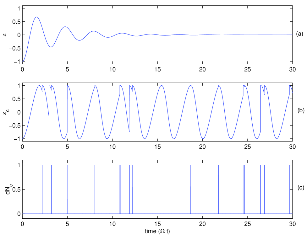
Fig. 2(a) shows the unconditional (ensemble average) time evolution of the population difference with the initial qubit state being in state , i.e., dot 1 is occupied . The unconditional population difference , rises from , undergoing some oscillations, and then tends towards zero, a steady (maximally mixed) state. On the other hand, the conditional time evolution, conditioned on one possible individual realization of the sequence of measurement results, behaves quite differently. We consider first the situation, where , discussed in Ref. [7]. In this case, due to the electrostatic repulsion generated by the electron, the PC is blocked (no electron is transmitted) when dot 1 is occupied. As a consequence, whenever there is a detection of an electron tunneling through the PC barrier, the qubit state is collapsed into state , i.e., dot 2 is occupied. The quantum-jump conditional evolution shown in Fig. 2(b) (using the same parameters and initial condition as in Fig. 2(a)) is rather obviously different from the unconditional one in Fig. 2(a). The conditional time evolution is not smooth, but exhibits jumps, and it does not tend towards a steady state. One can see that initially the system starts to undergo an oscillation. As the population difference changes in time, the probability for an electron tunneling through the PC barrier increases. This oscillation is then interrupted by the detection of an electron tunneling through the PC barrier, which bring to the value , i.e., the qubit state is collapsed into state . Then the whole process starts again. The randomly distributed moments of detections, , corresponding to the quantum jumps in Fig. 2(b) is illustrated in Fig. 2(c). Although little similarity can be observed between the time evolution in Fig. 2(a) and (b), averaging over many individual realizations shown in Fig. 2(b) leads to a closer and closer approximation of the ensemble average in Fig. 2(a).
Next we illustrate how the transition from the quantum-jump picture to the quantum-diffusive picture takes place. In Ref. [15] and Sec. III, we have seen that the quantum-diffusive equations can be obtained from the quantum-jump description under the assumption of . In Fig. 3(a)–(d) we plot conditional, quantum-jump evolution of and the corresponding moments of detections , with different ratios. Each jump (discontinuity) in the curves corresponds to the detection of an electron through the PC barrier. One can clearly observes that with increasing ratio, the number of jumps increases. The amplitudes of the jumps of , however, decreases from with the certainty of the qubit being in state to the case of with a smaller probability of finding the qubit in state . Nevertheless, the population difference always jumps up since . In other words, whenever there is a detection of an electron passing through PC, dot 2 is more likely occupied than dot 1. The case for quantum diffusion using Eq. (IV) is plotted in Fig. 3(e). In this case, very small jumps occur very frequently. We can see that the behavior of for in the quantum-jump case shown in Fig. 3(d) is already very close to that of quantum diffusion shown in Fig. 3(e). To minimize the number of controllable variables, the same randomness is applied to produce the quantum-jump, conditional evolutions in Fig. 3(a)–(d). This, however, does not mean that they would have had the same detection output, . The number of tunneling events in time , , does not depend on the randomness alone. It also depends on , , and , and has to satisfy Eq. (21) in a self-consistent manner. In fact, it both conditions and is conditioned by the conditional qubit density matrix. Note that the unconditional evolution does not depend on the parameter when (see Eq. (IV)). This implies that depending on the actual measured detection events, different measurement schemes (measurement devices with different tunneling barriers or different values of when ) give different conditional quantum evolutions. But they would have the same ensemble average property if other parameters and the initial condition are the same. Hence, averaging over all possible realizations, for each measurement scheme in Fig. 3, will lead to the same ensemble average behavior shown in Fig. 2(a).
B Quantum Zeno effect
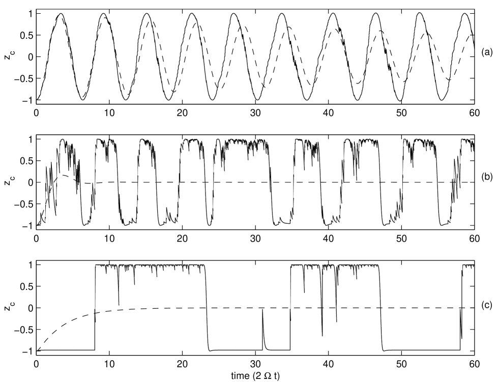
The quantum Zeno effect can be naturally described by the conditional dynamics. The case for quantum diffusion has been discussed in Ref. [8, 10]. Here, for completeness, we discuss the quantum-jump case. The quantum Zeno effect states that repeated observations of the system slow down transitions between quantum states due to the collapse of the wave function into the observed state. Alternatively, the interaction with one measurement apparatus destroys the quantum coherence (oscillations) between and at a rate that is much faster than the tunneling rate . For fixed , and , by increasing the interaction with the PC detector , we increase the number and amplitude of jumps and hence the probability of the wave function being collapsed to the localized state. The time evolutions of the population difference for different ratios of are shown in Fig. 4. Here, the initial qubit state is , and other parameters are: , , , . We can observe that the period of coherent oscillations between the two qubit states increases with increasing , while the time of a transition (switching time) decreases. In the limit of vanishing , a transition from one qubit state to the other state takes a time (switching time) of order of localization time [15], . In the parameter regime of Fig. 4(c) (), this time is still much smaller than the average time between state-changing transitions (period of oscillations) due to , i.e., the mixing time [15], . Hence, we can already see from Fig. 4(c) for that very frequent repeated measurements would tend to localize the system.
The ensemble average behavior of is also shown in dashed line in Fig. 4. If and initially the electron is in dot 1, from the solution of Eq. (II) , the probability can be written as
| (57) |
where . In the Appendix, the stationary noise power spectrum of the current fluctuations through the PC barrier is calculated for the case of and the result can be written as [10]:
| (58) |
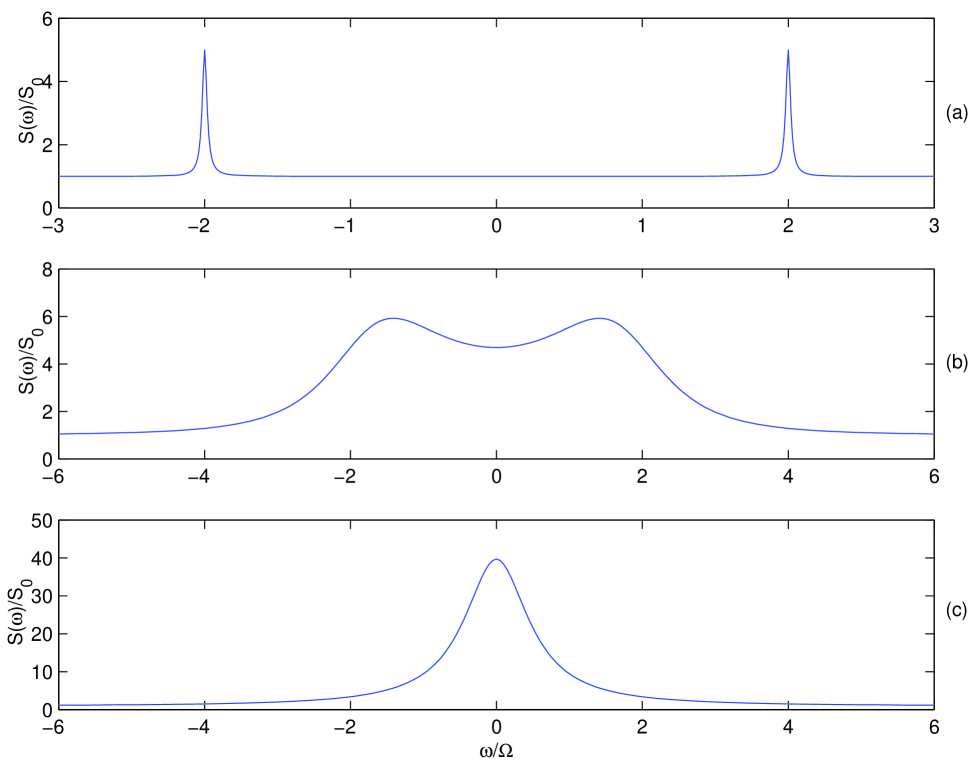
where represents the shot noise, is the steady-state current and represents the difference between the two average currents. For , shows the damped oscillatory behavior in the immediate time regime (see dashed line in Fig. 4(a) and (b)). In this case, the spectrum has a double peak structure, indicating that coherent tunneling is taking place between the two qubit states. This is illustrated in Fig. 5(a) and (b). When , does not oscillate but decays in time purely exponentially, saturating at the probability . (see dashed line in Fig. 4(c)) This corresponds to a classical, incoherent behavior. In this case, only a single peak, centering at , appears in the noise spectrum, as illustrated in Fig. 5(c). The evolution of in Fig. 4(c), is one of the possible conditional evolutions in this parameter regime (). In this parameter regime , the conditional evolution behaves very close to a probabilistic jumping or random telegraph process. After ensemble averaging over all possible realizations of such conditional evolutions, one would then obtain the classical, incoherent behavior.
C Relative phase of the tunneling amplitudes
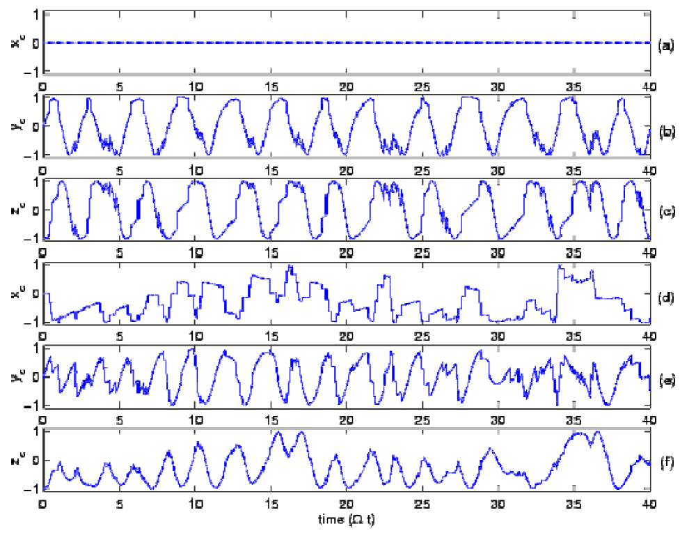
The relative phase between the two complex tunneling amplitudes produces effects on both conditional and unconditional dynamics of the qubit. In the following, we consider the case that and . From Eq. (IV), after each jump the imaginary part of the product seems to cause an additional rotation around the -axis in the Bloch sphere, but does not directly change the population probability of the qubit. However, the actual conditional evolution of the Bloch sphere variables is complicated. It is stochastic and nonlinear, and depends on the relative phase of the tunneling amplitudes in a nontrivial way. Nevertheless, after ensemble average, the imaginary part of generates an effective shift in the energy mismatch of the qubit states (see Eq. (II)).
There are situations in which the effect of the relative phase of the tunneling amplitudes can be easily seen. For and , if the tunneling amplitudes are real, i.e., , and the initial condition , then the time evolution of , from Eq. (IV), does not change and remains at the value at all times. But if or , the conditional evolution of behaves rather differently. It changes after the first detection (quantum jump) takes place. Fig. 6 shows the evolutions of the Bloch variables , , with the same initial condition (the qubit being in ) and parameters but different relative phases: for (a)–(c), and for (d)–(f). We can clearly see quite different behaviors of in these two cases. The asymmetry of the electron population in , due to effectively generated energy mismatch in the second case in Fig. 6(f), can be roughly observed. The effect of the relative phase is small in the case of quantum diffusion. As noted in Sec. III, in order for the quantum-diffusive equations to be valid, we should regard, to the order of magnitude, that and . This implies that in this case . Hence the effect of the relative phase is small and the conditional dynamics does not deviate much from the case that the tunneling amplitudes are assumed to be real[8, 10, 14].
D Inefficient measurement and non-ideality
We have shown [15] that for , the conditional time evolution of the qubit can be described by a ket state vector satisfying the stochastic Schrödinger equation. It is then obvious that perfect detection or efficient measurement preserves state purity for a pure initial state. However, the inefficiency and non-ideality of the detector spoils this picture. The decrease in our knowledge of the qubit state leads to partial decoherence for the qubit state. We next find the partial decoherece rate introduced in this way.
The stochastic differential equations in the form of Itô calculus [39, 40] have the advantage that it is easy to see that the ensemble average of the conditional equations over the random process leads to the unconditional equations. However, it is not a natural physical choice. For example, for , the term in Eq. (33) does not really cause decoherence of the conditional qubit density matrix. It simply compensates the noise term due to the definition of derivative in Itô calculus. Hence, in this case the conditional evolution of does not really decrease in time exponentially. To find the partial decoherence rate generated by inefficiency , we transform Eq. (33) into the form of Stratonovich calculus [39, 40]. We then obtain for :
| (59) |
where . Here we have used the following relations: the conditional current with given by Eq. (26) and the average current , where and in the quantum-diffusive limit. In this form, Eq. (59) elegantly shows how the qubit density matrix is conditioned on the measured current. We find that the last term in Eq. (59) is responsible for decoherence. In other words, the partial decoherence rate for an individual realization of inefficient measurements is . For a perfect detector , this decoherence rate vanishes and the conditional , as expected, does not decay exponentially in time. Similar conclusion could be drawn from Eq. (IV) for the quantum-jump case. For , the off-diagonal variables and seem to decrease in time with the rate .
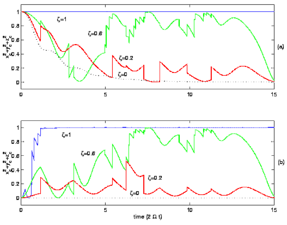
In Bloch sphere variable representation, we can use the quantity as a measure of the purity of the qubit state, or equivalently as a measure of how much information the conditional measurement record gives about the qubit state. If the conditional state of the qubit is a pure state then ; if it is a maximally incoherent mixed state then . We plot in Fig. 7 the quantum-jump, conditional evolution of the purity for different inefficiencies, , , (in solid line), and (in dotted line). Fig. 7(a) is for a initial qubit state being in a pure state , while Fig. 7(b) is for a maximally mixed initial state. We can see from Fig. 7(a) that the purity at all times for , while it hardly or not at all reaches for almost all time for . This means that partial information about the changes of the qubit state is lost irretrievably in inefficient measurements. In addition, roughly speaking, the overall behavior of decreases with decreasing . This indicates that after being averaged over a long period of time, would also decrease with decreasing . For , the evolution of becomes smooth and tends toward the value zero (the maximally mixed steady state). For a non-pure initial state (see Fig. 7(b)), the qubit state is eventually collapsed towards a pure state and then remains in a pure state for . But the complete purification of the qubit state cannot be achieved for . As in Fig. 3(a)–(d), the same randomness has been applied to generate the quantum-jump, conditional evolution in Fig. 7(a) and (b). Note that the only difference between evolution in Fig. 7(a) and the corresponding one in Fig. 7(b) is the different initial states. So when the qubit density matrix in Fig. 7(b) gradually evolves into the same state as in Fig. 7(a), the corresponding in Fig. 7(b) would then follow the same evolution as in Fig. 7(a). This behavior can be observed in Fig. 7. The purity-preserving conditional evolution for a pure initial state, and gradual purification for a non-pure initial state for an ideal detector have been discussed in Refs. [8, 9, 10, 13] in the quantum-diffusive limit.
The non-ideality of the PC detector is modeled in Refs. [8, 9, 10, 13] by another ideal detector “in parallel” to the original one but with inaccessible output. We can add, as in Refs. [8, 9, 10, 13], an extra term, , to Eq. (59) to account for the “non-ideality” of the detector. The ideal factor introduced there [8, 9, 10, 13] can be modified to take account of inefficient measurement discussed here. We find
| (60) |
where and . For , we have . In Ref. [14], inefficient measurement is discussed in terms of insufficiently small readout period. As a result, the information about the tunneling times of the electrons passing through the PC barrier is partially lost.
V Conclusion
We have obtained the quantum-jump and quantum-diffusive, conditional master equations for the case of inefficient measurements. These conditional master equations describe the random evolution of the measured qubit density matrix, which both conditions and is conditioned on, a particular realization of the measured current. We have analyzed the conditional qubit dynamics in detail and illustrated the conditional evolution by numerical simulations. Specifically, the conditional qubit dynamics evolving from quantum jumps to quantum diffusion has been presented. Furthermore, we have described the quantum Zeno effect in terms of the quantum-jump, conditional dynamics. We have also discussed the effect of inefficient measurement and the influence of relative phase between the two tunneling amplitudes on the qubit dynamics.
Acknowledgment
H.S.G. is grateful for useful discussions with A. N. Korotkov, G. Schön, D. Loss, Y. Hirayama, J. S. Tsai and G. P. Berman. H.S.G. would like to thank H. B. Sun and H. M. Wiseman for their assistance and discussions in the early stage of this work.
A Calculation of the noise power spectrum of the current fluctuations
In this Appendix, we calculate the stationary noise power spectrum of the current fluctuations through the PC when there is the possibility of coherent tunneling between the two qubit states. Usually one can calculate this noise power spectrum using the unconditional, determistic master equation approach, which gives only the average characteristics. We, however, calculate it through the stochastic formalism presented here. The fluctuations in the observed current, , are quantified by the two-time correlation function:
| (A1) |
The noise power spectrum of the current is then given by
| (A2) |
The ensemble expectation values of the two-time correlation function for the current in the case of quantum diffusion has been calculated in Ref. [10]. Here we will present the quantum-jump case. The current in this case is given by Eq. (18). We will follow closely the calculation in the Appendix of Ref. [28] to calculate the two-time correlation function, . First we consider the case when , where is the minimum time step considered. Since is a classical point process, it is either zero or one. As a result, is non-vanishing only if there is electron-tunneling event inside each of these two infinitesimal time intervals, and . Hence, we can write
| (A3) |
where the subscript to the vertical line is the condition for which the subscript on exists. From Eqs. (21) and (22), we have and . Using the fact that and Eqs. (7) and (22), we can write
| (A4) | |||||
| (A5) |
Hence, to leading order in , we obtain for :
| (A6) |
For , we have, from Eq. (18), that:
| (A7) |
For short times, this term dominates and we may regard as -correlated noise for a suitably defined function. Thus the current-current two-time correlation function for can be written as:
| (A8) | |||||
| (A9) |
In this form, we have related the ensemble averages of classical random variable to the quantum averages with respect to the qubit density matrix. The case is covered by the fact that the current-current two-time correlation function or is symmetric in , i.e., .
Next we calculate steady-state and . We can simplify Eq. (A9) using the following identities for an arbitrary operator : , , and , where the subscript indicates that the system is at the steady state and the steady-state density matrix is a maximally mixed state. Hence we obtain the steady-state for as:
| (A10) |
where the steady-state average current . The first term in Eq. (A10) represents the shot noise component. It is easy to evaluate Eq. (A10) analytically for case. The case for the asymmetric qubit, , can be calculated numerically. Evaluating Eq. (A10) for , we find
| (A11) |
where , and we have represented as the difference between the two average currents. After Fourier transform following from Eq. (A2), the power spectrum of the noise is then obtained as the expression of Eq. (58). Note that from Eq. (58), the noise spectrum at for , i.e., real tunneling amplitudes, can be written as:
| (A12) |
where represents the shot noise. In obtaining Eq. (A12), we have used the relation for the case of real tunneling amplitudes. In the quantum-diffusive limit or , this ratio , independent [10] of the values of and . These results for and in the limit of quantum diffusion are consistent with those derived in Ref. [10] using both the unconditional master equation approach and conditional stochastic formalism with white noise current fluctuations for an ideal detector.
REFERENCES
- [1] E-mail: goan@physics.uq.edu.au.
- [2] B. E. Kane, Nature, 393, 133 (1998). V. Privman, I. D. Vagner, and G. Kventsel, Phys. Lett. A 239, 141 (1998).
- [3] D. Loss and D. P. DiVincenzo, Phys. Rev. A 57, 120 (1998). A. Imamoglu, D. D. Awschalom, G. Burkard, D. P. DiVincenzo, B. D. Loss, M. Sherwin, and A. Small, Phys. Rev. Lett. 83, 4204 (1999).
- [4] A. Shnirman, G. Schön, and Z. Hermon, Phys. Rev. Lett. 79, 2371 (1997); D. V. Averin, Solid State Commun. 105, 659 (1998).
- [5] N. H. Bonadeo, J. Erland, D. Gammon, D. Park, D. S. Katzer, and D. G. Steel, Science 282, 1473 (1998).
- [6] S. A. Gurvitz, Phys. Rev. B 56, 15215 (1997).
- [7] S. A. Gurvitz, quant-ph/9808058.
- [8] A. N. Korotkov, Phys. Rev. B 60, 5737 (1999).
- [9] A. N. Korotkov, Physica B 280, 412 (2000).
- [10] A. N. Korotkov, cond-mat/0003225.
- [11] Y. Makhlin, G. Schön, and A. Shnirman, cond-mat/9811029; cond-mat/0011269.
- [12] Y. Makhlin, G. Schön, and A. Shnirman, Phys. Rev. Lett. 85, 4578 (2000).
- [13] A. N. Korotkov, cond-mat/0008003.
- [14] A. N. Korotkov, cond-mat/0008461.
- [15] H.-S. Goan, G. J. Milburn, H. M. Wiseman, H. B. Sun, to appear in Phys. Rev. B, cond-mat/0006333.
- [16] I. L. Aleiner, N. S. Wingreen, and Y. Meir, Phys. Rev. Lett. 79, 3740 (1997).
- [17] Y. Levinson, Europhys. Lett. 39, 299 (1997).
- [18] L. Stodolsky, Phys. Lett. B 459, 193 (1999).
- [19] M. Büttiker and A. M. Martin, Phys. Rev. B 61, 2737 (2000).
- [20] G. Hackenbroich, B. Rosenow, and H. A. Weidenmüller, Phys. Rev. Lett. 81, 5896 (1998).
- [21] D. V. Averin, cond-mat/0004364; A. N. Korotkov and D. V. Averin, cond-mat/0002203.
- [22] A. Shnirman and G. Schön, Phys. Rev. B 57, 15400 (1998).
- [23] D. V. Averin, cond-mat/0008114; cond-mat/0010052.
- [24] A. Maassen van den Brink, cond-mat/0009163.
- [25] H. J. Carmichael, An Open System Approach to Quantum Optics, Lecture notes in physics (Springer, Berlin, 1993).
- [26] J. Dalibard, Y. Castin, and K. Molmer, Phys. Rev. Lett. 68, 580 (1992).
- [27] N. Gisin and I. C. Percival, J. Phys. A 25 5677 (1992); 26 2233 (1993); 26 2245 (1993).
- [28] H. M. Wiseman and G.J. Milburn, Phys. Rev. A 47, 1652 (1993).
- [29] M. J. Gagen, H. M. Wiseman, and G. J. Milburn, Phys. Rev. A 48, 132 (1993).
- [30] G. C. Hegerfeldt, Phys. Rev. A 47, 449 (1993).
- [31] H. M. Wiseman, Quantum Semiclass. Opt. 8, 205 (1996).
- [32] C. Presilla, R. Onofrio, and U. Tambini, Ann. Phys. 248, 95 (1996).
- [33] M. B. Mensky, Phys. Usp. 41, 923 (1998).
- [34] M. B. Plenio and P. L. Knight, Rev. Mod. Phys. 70, 101 (1998).
- [35] C. W. Gardiner and P. Zoller, Quantum Noise, 2nd ed. (Springer, Berlin, 2000).
- [36] The finite-temperature unconditional master equation for the CQD system, taking into account the effect of thermal PC reservoirs under the weak system-environment coupling and Markovian approximations, is obtained in Ref. [15].
- [37] H. M. Wiseman and G. J. Milburn, Phys. Rev. A 47, 642 (1993).
- [38] G. Lindblad, Comm. Math. Phys. 48, 119 (1973).
- [39] G. W. Gardiner, Handbook of Stochastic Method (Springer, Berlin, 1985).
- [40] B. Øksendal, Stochastic Differential Equations (Springer, Berlin, 1992).
- [41] H.-S. Goan and G. J. Milburn, submitted to the Proceedings of International Conference on Experimental Implementations of Quantum Computing, Sydney, Australia (Rinton Press, 2001), cond-mat/0102058.