[

Devil’s Staircase in Magnetoresistance of a Periodic Array of Scatterers

Abstract

The nonlinear response to an external electric field is studied for classical non-interacting charged particles under the influence of a uniform magnetic field, a periodic potential, and an effective friction force. We find numerical and analytical evidence that the ratio of transversal to longitudinal resistance forms a Devil’s staircase. The staircase is attributed to the dynamical phenomenon of mode-locking.

]

The electron transport in two-dimensional periodic arrays of scatterers has been actively studied for the last decade. One of the most interesting feature is the plateau-like behaviour in Hall resistance as well as peaks in magnetoresistance[1, 2] at low magnetic fields below the quantum Hall regime. The peak structure in magnetoresistance has been attributed to the electron cyclotron orbits which enclose an integer number of scatterers [2, 3]. The cyclotron motion is important when the electron mean free path $l$ ($l$ is measured in the absence of periodic scatterers) is greater than the period $a$ of the regular scatterers.

In this Letter, we present a theory for electron transport in the deeply diffusive regime $l\ll a$ where cyclotron motion is not relevant. We predict a new and interesting effect where the structure in the magnetoresistance is associated with fractional numbers. We will show that the relative ratio between the transversal and longitudinal magnetoresistance forms a Devil’s staircase. These fractal staircases originate from a dynamical phenomenon known as mode-locking which appears naturally in the context of circle maps [4]. Our prediction is based on the finding that the dynamics in a two-dimensional periodic array of scatterers with intrinsic momentum relaxation effectively reduces to a circle map.

Let us consider first a particle of mass $m$, charge $q$ in crossed electric (${\mbox{\boldmath$E$\unboldmath}}=E\hat{\mbox{\boldmath$x$\unboldmath}}$) and magnetic fields (${\mbox{\boldmath$B$\unboldmath}}=-B\hat{\mbox{\boldmath$z$\unboldmath}}$) with intrinsic momentum relaxation. The resulting drift motion ${\mbox{\boldmath$x$\unboldmath}(t)}=(x(t),y(t))$ can be described by adding a frictional force, proportional to the drift velocity $v$, to the equations of motion yielding

$$\dot{x}=v_{x} \quad m\dot{v}_{x}=-qBv_{y}+qE-mv_{x}/\tau$$ , (1)

$$\dot{y}=v_{y} \quad m\dot{v}_{y}=qBv_{x}-mv_{y}/\tau$$ , (2)

with $\tau$ being the momentum relaxation time. Cyclotron motion only exists for a transient time; each trajectory finally converges to a straight line ${\mbox{\boldmath$x$\unboldmath}}(t\to\infty)={\mbox{\boldmath$x$\unboldmath}}(0)+\langle{\mbox{\boldmath$v$\unboldmath}}\rangle t$, with the time-averaged velocity $\langle{\mbox{\boldmath$v$\unboldmath}}\rangle=(m/\tau,qB)qE/(q^{2}B^{2}+m^{2}/\tau^{2})$. With the charge density $n$ and the current density ${\mbox{\boldmath$J$\unboldmath}}=qn\langle{\mbox{\boldmath$v$\unboldmath}}\rangle$, it is easy to calculate the resistivities defined by ${\mbox{\boldmath$E$\unboldmath}}=\hat{\rho}{\mbox{\boldmath$J$\unboldmath}}$ and Onsager’s relations $\rho_{xx}=\rho_{yy}$ and $\rho_{yx}=-\rho_{xy}$: the diagonal resistivity $\rho_{xx}=m/q^{2}n\tau$ is constant, whereas the off-diagonal resistivity $\rho_{xy}=B/qn$ depends linearly on the magnetic field – no plateaus are present.

We now add a periodic potential $V=V_{0}F({\mbox{\boldmath$x$\unboldmath}})$ with $|F|$ of order one to the equations of motion (1), assuming that the periodicity of the potential, $a$, is much larger than the length scale related to the intrinsic momentum relaxation. When we scale the coordinates $x$ with $a$ and the time $t$ with $\tau$, we get the same equations of motion for a given set of three dimensionless parameters: $\tilde{B}=q\tau B/m$, $\tilde{E}=q\tau^{2}E/(ma)$, and $\tilde{V}_{0}=V_{0}/(qEa)$. We use the rescaled magnetic field $\tilde{B}$ as a variable parameter and fix the rescaled electric field and potential strength to $\tilde{E}=15.3$ and $\tilde{V}_{0}=0.12$ if not otherwise stated. Though we could choose various sets of parameters ($\tau,a,E$, etc.) for the chosen values of $\tilde{E}$ and $\tilde{V}_{0}$, for definiteness we will take $\tau=7.6~{}10^{-14}s$, $E=-2.3~{}10^{4}V/cm$, and $a=0.5\mu m$, and fix these for the rest of the paper. The particle is an electron in GaAs sample with $q=-e$ and $m=0.067m_{e}$. By taking a typical value of Fermi velocity $v_{f}\approx 3\times 10^{7}cm/s$, the mean free path of our system is $l=v_{f}\tau\approx 0.02\mu m\ll a$.

First, we show how the particle’s motion is related to a one-dimensional circle map through analytical considerations for sufficiently small potential strength. Note that our numerics do not rely on this requirement. Due to the periodicity of the potential it is sufficient to consider the unit cell of the potential with periodic boundary conditions, i.e. we can compactify the $(x,y)$-plane to a two-dimensional torus. A typical asymptotic solution for zero potential strength as discussed above appears here as a quasiperiodic trajectory filling densely a two-dimensional invariant torus ${\mbox{\boldmath$v$\unboldmath}}=\mbox{constant}$ in four-dimensional phase space. Trajectories starting away from the torus are attracted towards it and asymptotically converge onto it. For finite potential strength the torus is smoothly deformed or collapsed into lower-dimensional objects or broadened to a higher-dimensional object (loosely speaking, a torus with finite but very small thickness). The latter possibility can be ignored to a very good approximation as we will see later. A point on the torus (and on the lower-dimensional objects) is uniquely labelled by unit-cell coordinates $(x_{1}\,{\rm mod}\,1,x_{2}\,{\rm mod}\,1)$ defined by ${\mbox{\boldmath$x$\unboldmath}}=x_{1}{\mbox{\boldmath$a$\unboldmath}}_{1}+x_{2}{\mbox{\boldmath$a$\unboldmath}}_{2}$, with ${\mbox{\boldmath$a$\unboldmath}}_{1}=(a_{11},a_{12})$, ${\mbox{\boldmath$a$\unboldmath}}_{2}=(a_{21},a_{22})$ being the lattice vectors of the unit cell. The long-time behavior is therefore completely described by two-dimensional dynamics $[x_{1}(t),x_{2}(t)]$. As usual, such dynamics can be conveniently investigated by introducing Poincaré surfaces of section defined by $x_{1}(t_{n})\,{\rm mod}\,1=0$, where $n$ is an integer and modulo 1 restricts the variable to the interval $[0,1)$.

The discrete evolution of $x_{2,n}\equiv x_{2}(t_{n})$ is then governed by a one-dimensional map $x_{2,n+1}=f(x_{2,n})$ where $f$ is a smooth and monotonic function. Due to the periodicity of the potential the condition $f(x_{2})\,{\rm mod}\,1=f(x_{2}\,{\rm mod}\,1)$ holds. Such a map is called an invertible circle map. Its rotation number,

$$\rho\equiv\lim_{n\to\infty}\frac{x_{2,n}-x_{2,0}}{n}\ ,$$ (3)

is well-defined and independent of the initial condition $x_{2,0}$ [4]. A rational value of $\rho=p/q$ ($p$ and $q$ are integers without common divisor) indicates periodic motion, whereas an irrational value indicates quasiperiodic motion; chaotic motion is not possible.

We now derive a simplified circle map valid in the limit $\tilde{V}_{0}\ll 1$. If $\tilde{V}_{0}=0$ then the asymptotic dynamics obeys $\dot{v}_{x}=\dot{v}_{y}=0$, leading to $f(x_{2})=x_{2}+\rho_{0}$ with the constant $\rho_{0}(\tilde{B})$; here we have simply $\rho=\rho_{0}$, so $\rho_{0}$ can be regarded as the unperturbed rotation number. The asymptotic dynamics for nonzero but sufficiently small $\tilde{V}_{0}$ is overdamped, i.e. $|\dot{v}_{x}|\ll|v_{x}|/\tau$ and $|\dot{v}_{y}|\ll|v_{y}|/\tau$. As in the potential-free case the number of differential equations reduces to two, enabling us to determine $f$ up to first order in $\tilde{V}_{0}$

$$f(x_{2,n};\rho_{0},\tilde{E},\tilde{V}_{0})\approx x_{2,n}+\rho_{0}+\tilde{V}_{0}\;g(x_{2,n};\rho_{0})$$ (4)

with

$$g = \frac{\rho_{0}^{2}(a_{22}^{2}+a_{21}^{2})+2\rho_{0}(a_{11}a_{21}+a_{12}a_{22})+a_{12}^{2}+a_{11}^{2}}{(a_{11}a_{22}-a_{21}a_{12})^{2}}\times$$ (6)

$$\int_{0}^{1}\left(a_{21}\frac{\partial F}{\partial x_{1}}-a_{11}\frac{\partial F}{\partial x_{2}}\right)\Big{|}_{x_{2}=\rho_{0}x_{1}+x_{2,n}}dx_{1}\ .$$

$g$ is a nontrivial periodic function of $x_{2,n}$. Note that $f$ is independent of the parameter $\tilde{E}$ in the present approximation. Using Stoke’s theorem it can be shown that $\int_{0}^{1}gdx_{2}=0$. For circle maps of the form given in Eq. (4) with the above-mentioned properties of $g$ it is proven that for each $\tilde{V}_{0}$ there exists a Devil’s staircase, a monotonically increasing function $\rho=\rho(\rho_{0})$ with plateaus around each rational value of $\rho_{0}$. The width of the plateaus, $\Delta\rho_{0}$, is proportional to $\tilde{V}_{0}$ [5]. Similarly, the widths of the plateaus, $\Delta\tilde{B}$, of the function $\rho=\rho(\tilde{B})$, are proportional to $\tilde{V}_{0}$ since $\Delta\tilde{B}\approx(d\tilde{B}/d\rho_{0})\Delta\rho_{0}$.

The rotation number $\rho$ is directly related to the continuous-time dynamics. This can be seen by rewriting Eq. (3) with ${\mbox{\boldmath$v$\unboldmath}}=v_{1}{\mbox{\boldmath$a$\unboldmath}}_{1}+v_{2}{\mbox{\boldmath$a$\unboldmath}}_{2}$ as

$$\rho=\frac{\langle v_{2}\rangle}{\langle v_{1}\rangle}=\frac{-a_{12}+a_{11}\langle v_{y}\rangle/\langle v_{x}\rangle}{a_{22}-a_{21}\langle v_{y}\rangle/\langle v_{x}\rangle}=\frac{-a_{12}+a_{11}\sigma_{xy}/\sigma_{xx}}{a_{22}-a_{21}\sigma_{xy}/\sigma_{xx}}\ .$$ (7)

Hence, $\rho$ is given by the ratio of the conductivities. In the case that the periodic potential is invariant under $\pi/m$-rotations, $m=2,3,\ldots$, Onsager’s relations show that $\rho$ can also be expressed by the ratio $\rho_{xy}/\rho_{xx}$.

We now present numerical evidence showing that for finite $\tilde{V}_{0}\leq 0.4$ the continuous-time dynamics is indeed given by a one-dimensional circle map and that the magnetoresistance shows a fractal structure. As an example of the periodic scatterers, we take a potential with hexagonal symmetry shown in Fig. 1a,

$$V(x,y) = V_{0}\left\{\left[\cos\left(\frac{\pi}{3}(\sqrt{3}x-y)\right)\cos\left(\frac{2\pi}{3}y\right)\right]^{\beta}\right.$$ (8)

$$+ \left[\cos\left(\frac{\pi}{3}(\sqrt{3}x+y)\right)\cos\left(\frac{\pi}{3}(\sqrt{3}x-y)\right)\right]^{\beta}$$ (9)

$$+ \left.\left[\cos\left(\frac{2\pi}{3}y\right)\cos\left(\frac{\pi}{3}(\sqrt{3}x+y)\right)\right]^{\beta}\right\}\ ,$$ (10)

with $\beta=8$. The lattice vectors are ${\mbox{\boldmath$a$\unboldmath}}_{1}=(\sqrt{3},0)$ and ${\mbox{\boldmath$a$\unboldmath}}_{2}=(-\sqrt{3}/2,-3/2)$. We have used the Runge-Kutta method [6] with $10^{6}$ time steps of variable size to integrate the equations of motion. We found that all initial conditions, for fixed parameters, lead to the same mean velocity $\langle{\mbox{\boldmath$v$\unboldmath}}\rangle$. So only one single orbit is needed to calculate the current density and the resistivities without employing the Kubo formula [7]. This already indicates the collapse to an invertible circle map. To show the reduction to the map explicitly, we calculate a sequence of points $(x_{2,n}\,{\rm mod}\,1,x_{2,n+1}\,{\rm mod}\,1)$ by solving the complete set of differential equations for different initial velocities from one Poincaré section to the next. Figures 2a and b show that these points indeed lie very close to a line, so $x_{2,n+1}$ is to excellent approximation a function of $x_{2,n}$ independent of the initial velocity. We have computed $(x_{2,n+1}-x_{2,n}-\rho_{0})/\tilde{V}_{0}$ for different parameters $\tilde{V}_{0}$ and $\tilde{E}$. It can be seen from Fig. 2c that this quantity is roughly independent of $\tilde{V}_{0}$, even though small deviations indicate weak nonlinear behavior in $\tilde{V}_{0}$. Figure 2d shows that $(x_{2,n+1}-x_{2,n}-\rho_{0})/\tilde{V}_{0}$ does not change when $\tilde{E}$ is varied over two orders of magnitude. Figures 2a-d therefore confirm the reduction to the circle map and its parameter dependence as predicted in Eq. (4).

FIG. 1.: a) Contourplot of the potential in Eq. (8) with $\beta=8$. b) Orbit with $B=8.7T$ and $\rho=1$ in the unit cell. c) $B=9.77T$ and $\rho=1$. d) $9.8T$ and $\rho=1.01407...$. e) $2.9T$ and $\rho=1/2$. f) $4.4T$ and $\rho=2/3$.

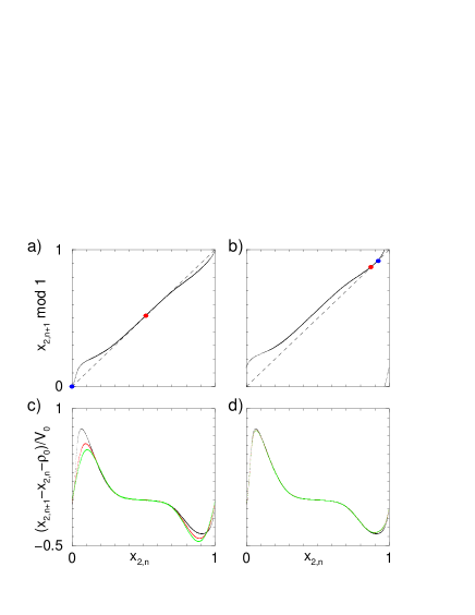
FIG. 2.: a) $x_{2,n+1}\,{\rm mod}\,1$ vs. $x_{2,n}$ for $B=8.7T$. b) $9.77T$. c) $(x_{2,n+1}-x_{2,n}-\rho_{0})/\tilde{V}_{0}$ vs. $x_{2,n}$ for $B=8.7T$, $\tilde{V}_{0}=0.12$ and $\tilde{E}=15.3$ (black); $\tilde{V}_{0}=0.06$ (red); $\tilde{V}_{0}=0.03$ (green). d) $\tilde{V}_{0}=0.12$ and $\tilde{E}=15.3$ (black); $\tilde{E}=1.53$ (red); $\tilde{E}=0.153$ (green).

Figure 3 is our main result. It shows the Devil’s staircase $\rho$ vs. $\rho_{0}$. Both quantities are computed from the resistivities via the relations $\rho=2/(1+\sqrt{3}\rho_{xx}/\rho_{xy})$ and $\rho_{0}=2/(1-\sqrt{3}/\tilde{B})$ from Eq. (7) with the lattice vectors of the rotational symmetric potential (8). Note the exactness of the plateaus. Let us discuss some features of the Devil’s staircase in relation to the continuous and discrete-time dynamics. Figures 1b and c show two orbits moving in slightly different magnetic fields. Both have synchronized velocities $\langle v_{1}\rangle=\langle v_{2}\rangle$, i.e. $\rho=1$. Each orbit with $\rho=1$ is a stable fixed point $x_{2}^{*}=f(x_{2}^{*})$ in the corresponding map (red circles in Figs. 2a and b; blue circles mark unstable fixed points). This synchronization phenomenon, usually called mode-locking in nonlinear dynamics, is therefore due to the robustness of fixed points under variation of a parameter, here $\rho_{0}(B)$. Orbits with $\rho\neq 1$ are in a different mode; in particular, orbits with irrational rotation number are not periodic. In Fig. 1d we see an orbit with irrational $\rho$ close to one. It stays for a long time near a periodic orbit with $\rho=1$ but from time to time it escapes, thereby filling the entire unit cell densely. This phenomenon is called intermittency [8]. In terms of the circle map, the transition from $\rho=1$ to irrational $\rho$ is a saddlenode bifurcation: as $B$ is varied, stable and unstable fixed points come closer and closer as illustrated in Figs. 2a and b, and finally destroy each other, yielding quasiperiodic motion. Varying $B$ further can lead again to periodic motion. Figures 1e and f give two examples with $\rho=1/2$ and $\rho=2/3$. The corresponding map has a stable fixed point of higher period, e.g. for $\rho=1/2$ the fixed point condition is $x_{2}^{*}=f[f(x_{2}^{*})]$.

FIG. 3.: Rotation number $\rho$ vs. $\rho_{0}$. Arrows assign the rational value of the rotation number $\rho=p/q$ to each plateau. The inset highlights the fractal structure of the Devil’s staircase.

We also observe a Devil’s staircase-like function $\rho_{xy}(B)$ in Fig. 4, which reminds one of the quantum Hall effects [9, 10], but here the ‘plateaus’ are not perfectly flat. One may note also that the way $\rho_{xx}$ varies for a number of $\rho_{xy}$-‘plateaus’ has similarities to the quantum Hall effects: going from the centre of a $\rho_{xy}$-‘plateau’ towards its border, $\rho_{xx}$ increases and reaches its maximum exactly when the ‘plateau’ ends. This can be explained qualitatively. First, note that an orbit from the centre of the $\rho=1$-plateau (Fig. 1b) avoids the potential’s steep maxima at the corners of the unit cell. Hence, the diagonal resistivity roughly equals the potential-free value $\rho_{xx}=m/q^{2}n\tau\approx 3.12k\Omega$. We infer from Figs. 1b and c that the closer $B$ is to the border of the plateau the closer is the orbit to the potential’s maxima. This effectively slows down the orbit, which explains the increase of $\rho_{xx}$ (and $\rho_{xy}$). Leaving the plateau finally reduces the resistivities because the intermittency effect becomes less pronounced with increasing $|\rho-1|$; see Fig. 1d.

FIG. 4.: Off-diagonal resistivity $\rho_{xy}$ and diagonal resistivity $\rho_{xx}$ vs. magnetic field $B$. Arrows assign the rational value of the rotation number $\rho=p/q$ to each plateau.

The example in Fig. 5 confirms that the widths of the plateaus, $\Delta B$, is roughly proportional to $\tilde{V}_{0}$ as predicted from the analysis of the simplified circle map in Eq. (4). By noting that $\tilde{V_{0}}$ denotes the dimensionless potential strength we see an interesting analogy with the quantum Hall effect where the size of plateaus is sensitive to the disorder strength of the systems [11]. Here we have the advantage of the use of the simplified circle map to analyse the plateau size, although the overall structure of the hierarchy of the plateaus is also too complicated to be dealt with in an analytic fashion.

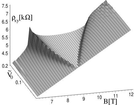
FIG. 5.: Dependence of the $\rho=1$-plateau on $\tilde{V}_{0}$; cf. Fig. 4.

Since the particle can be trapped in the very flat local minima of the potential (8), a finite dc electric field is necessary to overcome the potential trap as in the experiment in Ref.[12]. The threshold[13] value $E_{T}$ of the electric field for the finite electrical current might be crudely estimated by $E_{T}\sim V_{0}/(qa)$, which is in agreement with our calculations (not shown). However, in reality the threshold electric field will be much smaller in the presence of the degenerate electron gas because the weak local trap potential will be screened[14]. While we have chosen in our numerical calculation a large electric field ($2.3~{}10^{4}$V/cm) and a low mobility of the sample ($\mu=e\tau/m\approx 20000cm^{2}/Vs$), the Devil’s staircase may be observed in a broad range of parameters. We also note that the specific form of the potential (8) is not relevant. However, the steepness of the potential influences the shape of the plateaus. Large steepness (large $\beta$) results in wide and curved plateaus. It should be mentioned also that the Devil’s staircase will not be seen in the conventional Hall bar where the electrical current is fixed along the bar and the induced Hall voltage is measured. To measure the electrical current in two-dimensional samples for fixed applied voltages, one needs to use metallic leads which span the entire length of two opposite edges of the sample [14].

In summary, we have calculated the magnetoresistance of a lateral surface superlattice with strong momentum relaxation where the cyclotron motion is not involved. Our calculations show a fractal plateau structure in the magnetoresistance which stems from purely classical nonlinear dynamics. We have explained our calculational results in terms of the theory of circle maps where the Devil’s staircase is already well understood.

We acknowledge helpful discussions with P. Fulde, K. v. Klitzing, R. Gerhardts, K. Richter and R. Klages.

REFERENCES

- [1] K. Ensslin and P. M. Petroff, Phys. Rev. B 41, 12307 (1990).
- [2] D. Weiss, M. L. Roukes, A. Menschig, P. Grambow, K. von Klitzing, and G. Weimann, Phys. Rev. Lett. 66, 2790 (1991).
- [3] R. Fleischmann, T. Geisel, and R. Ketzmerik, Phys. Rev, Lett. 68, 1367 (1992).
- [4] see, e.g., D. Arrowsmith and C. Place, An introduction to dynamical systems (Cambridge University Press, Cambridge, 1990).
- [5] G. R. Hall, SIAM J. Math. Anal. 15, 1075 (1984).
- [6] W. H. Press, B. P. Flannery, S. A. Teukolsky, and W. T. Vetterling, Numerical Recipes in C (Cambridge University Press, Cambridge, 1988).
- [7] R. Kubo, J. Phys. Soc. Jpn 12, 570 (1957).
- [8] see, e.g., E. Ott, Chaos in dynamical systems (Cambridge University Press, Cambridge, 1993).
- [9] K. von Klitzing, G. Dorda, and M. Pepper, Phys. Rev. Lett. 45, 494 (1980).
- [10] D. C. Tsui, H. L. Stormer, and A. C. Gossard, Phys. Rev. Lett. 48, 1559 (1982).
- [11] See e.g., M. Janssen, O. Viehweger, U. Fastenrath, and J. Hajdu, Introduction to the Theory of the Integer Quantum Hall Effect, (VCH Verlagsgesellschaft mbH, Weinheim, 1994).
- [12] G. M. Gusev, Z. D. Kvon, A. G. Pogosov, and M. M. Voronin, JETP Lett. 65, 248 (1997).
- [13] The threshold behavior is also seen in the charge-density-wave transport; see for a review, G. Grüner, Density Waves in Solids (Addison-Wesley, Reading, MA, 1994). Devil’s staircases appear in these systems if both ac and dc electric fields are applied; see P. Bak, T. Bohr, and M. H. Jensen, Physica Scripta T9, 50 (1985).
- [14] K. v. Klitzing, private communications.