In-plane upper critical field anisotropy in Sr₂RuO₄ and CeIrIn₅

Abstract

Experiments on tetragonal Sr₂RuO₄ and CeIrIn₅ indicate the presence of superconductivity with a multi-component superconducting order parameter. Such an order parameter should exhibit an in-plane anisotropy in the upper critical field near the superconducting transition temperature that does not occur for single-component superconductors. Here, this anisotropy is determined from microscopic calculations for arbitrary gap functions. It is shown that this anisotropy is generally not small and, in some cases, independent of impurity scattering. Furthermore, this anisotropy is calculated for many detailed microscopic models of Sr₂RuO₄. For these models this anisotropy is found to be large, which is in sharp contrast to the small anisotropy observed experimentally. However, an accidental cancellation of the anisotropy for gaps on different Fermi surface sheets can lead to a result that is consistent with experiment.

One of the central issues in the field of unconventional superconductivity is the identification of the order parameter symmetry. This issue can usually only be addressed by determinations of the phase of the order parameter (such as through Josephson junction experiments [1]). However, in the case that the Cooper pair wave functions have more than one complex degree of freedom, other experimental signatures can reveal the pairing symmetry. In this paper one of these signatures, the upper critical field anisotropy for fields in the basal plane, is explored for tetragonal superconductors. This anisotropy was established by Gor’kov on phenomenological grounds [2]. Such an anisotropy, for which $dH_{c2}/dT|_{T=T_{c}}$ is not equal for the magnetic field applied along the $(1,0,0)$ (along the crystallographic ${\bf a}$ axis) and the $(1,1,0)$ directions, cannot occur for superconducing order parameters that have only one complex degree of freedom (for example conventional $s$-wave superconductors or $d_{x^{2}-y^{2}}$-wave superconductors). Consequently, this provides a clear test of the pairing symmetry. For tetragonal materials, there exist two possible pairing states that exhibit this property. One is the spin triplet $E_{u}$ representation which can be described a gap function of the form (note that this is not the most general form) ${\bf d}({\bf k})=\hat{z}[\eta_{1}f_{x}({\bf k})+\eta_{2}f_{y}({\bf k})]$, where in the simplest case (for a cylindrical Fermi surface) $f_{x}({\bf k})=k_{x}$ and $f_{y}({\bf k})=k_{y}$. Such a gap function is believed to describe the pairing state in Sr₂RuO₄ (see below)[3, 4]. The other pairing state is the spin-singlet $E_{g}$ representation which can be described by a gap function of the form $\Psi({\bf k})=\eta_{1}f_{xz}({\bf k})+\eta_{2}f_{yz}({\bf k})$, where $f_{xz}({\bf k})=k_{x}k_{z}$ and $f_{yz}({\bf k})=k_{y}k_{z}$ in the simplest case. In this article, the anisotropy is determined within microscopic theories with arbitrary gap functions. It is shown that the anisotropy is generally not small and consequently easily observable. Furthermore, it is shown that for the $E_{g}$ representation and for some theories for the $E_{u}$ representation, this anisotropy is impurity independent. Application of these results to Sr₂RuO₄ and CeIrIn₅ are discussed and detailed calculations for Sr₂RuO₄ are also presented. Prior to discussing the anisotropy, an overview of the superconductivity in Sr₂RuO₄ and CeIrIn₅ is given.

The oxide Sr₂RuO₄ has a structure similar to high $T_{c}$ materials and was observed to be superconducting by Maeno et al. in 1994 [5]. It has been established that this superconductor is not a conventional $s$-wave superconductor: NQR measurements show no indication of a Hebel-Slichter peak [6] in $1/T_{1}T$, and $T_{c}$ is strongly suppressed below the maximum value of 1.5 K by non-magnetic impurities [7]. More recent experiments indicate an $E_{u}$ odd parity gap function of the form ${\bf d}({\bf k})=\hat{z}[\eta_{1}f_{x}({\bf k})+\eta_{2}f_{y}({\bf k})]$. The Knight shift measurements of Ishida et al. [8] reveal that the spin susceptibility is unchanged upon entering the superconducting state; this is consistent with $p$-wave superconductivity (as predicted by Rice and Sigrist [9] and Baskaran [10]). Furthermore, these measurements were conducted with the applied field in the basal plane. Since the orientation of the gap function (that is ${\bf d}$) is orthogonal to the spin projection of the Cooper pair [11], these measurements are consistent with the gap function aligned along the $\hat{z}$ direction. The $\mu$SR experiments of Luke et. al. have revealed spontaneous fields in the Meissner state [12]. This indicates that the superconducting order parameter must have more than one component [11, 12]. This leads naturally to the conclusion that the superconducting gap function has the form ${\bf d}({\bf k})=\hat{z}(f_{x}\pm if_{y})$. This conclusion is consistent with measurements of the field distribution of the vortex lattice [13], Josephson tunnelling experiments [14], and point-contact measurements [15]. One immediate consequence of such a gap function is that the resulting low energy excitation spectrum is gapless in the clean limit. However, recent experiments indicate this is not the case. Specific heat measurements [16], NQR measurements [17], and cavity penetration depth measurements [18] all indicate the presence of nodes in the superconducting gap function. This has prompted a recent series of proposals that the gap function has the form ${\bf d}({\bf k})=\hat{z}[\eta_{1}f_{x}({\bf k})+\eta_{2}f_{y}({\bf k})]$ where $f_{x}({\bf k}_{0})=f_{y}({\bf k}_{0})=0$ for a set of points ${\bf k}_{0}$ that form a line on the Fermi surface [19, 20, 21] or are very anisotropic [22, 23, 24, 25]. These gap functions are all formally of the same $E_{u}$ symmetry. The fact that these theories all have the same symmetry implies that there exist experimental signatures that will be common to all of them. In particular, the upper critical field anisotropy discussed above should exist. Recently, such an anisotropy has been observed by Mao et al.[26]. It was determined that $1-H_{c2}^{(100)}/H_{c2}^{(110)}=0.03$ at a temperature of $0.35K$ ($\approx T_{c}/5$), $1-H_{c2}^{(100)}/H_{c2}^{(110)}$ was observed to change sign as $T\rightarrow T_{c}$, and appears to remain small for $T$ near $T_{c}$. In this paper, the anisotropy near $T_{c}$ will be calculated for a variety of models.

Very recently, it has been reported that $\mu$SR experiments of Heffner et. al. have revealed spontaneous fields in the Meissner state of tetragonal CeIrIn₅ [27, 28]. Just as in the case for Sr₂RuO₄ above, this indicates that the superconducting order parameter must have more than one component [11, 12]. This leads naturally to the conclusion that the superconducting gap function is either of $E_{u}$ symmetry of of $E_{g}$ symmetry. Consequently, both pairing symmetries are considered in this article.

The free energy for the $E_{u}$ and $E_{g}$ representations of $D_{4h}$ is given by [11]

$$f= -\alpha|\vec{\eta}|^{2}+\beta_{1}|\vec{\eta}|^{4}/2+\beta_{2}(\eta_{1}\eta_{2}^{*}-\eta_{2}\eta_{1}^{*})^{2}/2$$ (1)

$$+\beta_{3}|\eta_{1}|^{2}|\eta_{2}|^{2}+\kappa_{1}|D_{x}\eta_{1}|^{2}+|D_{y}\eta_{2}|^{2}$$ (2)

$$+\kappa_{2}(|D_{y}\eta_{1}|^{2}+|D_{x}\eta_{2}|^{2})$$ (3)

$$+\kappa_{5}(|D_{z}\eta_{1}|^{2}+|D_{z}\eta_{2}|^{2})$$ (4)

$$+\kappa_{3}[(D_{x}\eta_{1})(D_{y}\eta_{2})^{*}+h.c.]$$ (5)

$$+\kappa_{4}[(D_{y}\eta_{1})(D_{x}\eta_{2})^{*}+h.c.]+h^{2}/(8\pi).$$ (6)

where $D_{j}=\nabla_{j}-\frac{2ie}{\hbar c}A_{j}$, ${\bf h}=\nabla\times{\bf A}$, and ${\bf A}$ is the vector potential. The stable homogeneous solutions are easily determined [11]. There are three phases: (a) $\vec{\eta}=(1,i)/\sqrt{2}$ ($\beta_{2}>0$ and $\beta_{2}>\beta_{3}/2$), (b) $\vec{\eta}=(1,0)$ ($\beta_{3}>0$ and $\beta_{2}<\beta_{3}/2$), and (c) $\vec{\eta}=(1,1)/\sqrt{2}$ ($\beta_{3}<0$ and $\beta_{2}<0$). The weak-coupling approximation predicts that phase (a) is stable since this phase minimizes the number of nodes in the order parameter [note that in exceptional circumstances phase (a) may be degenerate with phase (b) and (c) in the weak-coupling limit, for example in the theory of Ref. [29] for $|\nu|=1$].

For an external magnetic field applied in the basal plane, the upper critical field can be determined and is found to be [2, 11]

$$H_{c2}(\theta)=\frac{\alpha hc}{e\sqrt{2\kappa_{5}}\sqrt{\kappa_{2}+\kappa_{1}-\sqrt{(\kappa_{1}-\kappa_{2})^{2}\cos^{2}(2\theta)+(\kappa_{3}+\kappa_{4})^{2}\sin^{2}(2\theta)}}}$$ (7)

where $\theta$ is the angle between the magnetic field and the crystallographic ${\bf a}$ axis. From the above expression, the ratio of $H_{c2}$ for the field along the $(1,0,0)$ direction to that for the field along the $(1,1,0)$ direction is given by $H_{c2}^{(1,1,0)}/H_{c2}^{(1,0,0)}=\sqrt{(\kappa_{1}+\kappa_{2}-|\kappa_{3}+\kappa_{4}|)/2min(\kappa_{2},\kappa_{1})}$ where $min(\kappa_{2},\kappa_{1})$ means the minimum of $\kappa_{1}$ and $\kappa_{2}$. Note that Sigrist has also determined an additional anisotropy that occurs due to spin-orbit coupling [30]. This additional anisotropy introduces a correction to Eq. 7 that vanishes as $T\rightarrow T_{c}$, so it is not considered here.

Here, this anisotropy is determined in the weak-coupling approximation. This approximation is reasonable for Sr₂RuO₄ since $T_{c}/T_{F}\approx 10^{-4}$, however it is not clear whether or not this approximation is valid for CeIrIn₅. Using a gap function of the form ${\bf d}({\bf k})=\hat{z}[\eta_{1}f_{x}({\bf k})+\eta_{2}f_{y}({\bf k})]$ for the $E_{u}$ representation and introducing isotropic impurity scattering within a $T$-matrix approximation yields (the details will be given in a later publication)

$$\kappa_{1}= \frac{\pi N(0)}{2}\sum_{n\geq 0}\frac{1}{(\omega_{n}+\Gamma)^{3}}[\langle f_{x}^{2}v_{x}^{2}\rangle+\frac{\Gamma}{\omega_{n}}\langle f_{x}v_{x}\rangle^{2}]$$ (8)

$$\kappa_{2}= \frac{\pi N(0)}{2}\sum_{n\geq 0}\frac{1}{(\omega_{n}+\Gamma)^{3}}\langle f_{x}^{2}v_{y}^{2}\rangle$$ (9)

$$\kappa_{3}= \frac{\pi N(0)}{2}\sum_{n\geq 0}\frac{1}{(\omega_{n}+\Gamma)^{3}}\times$$ (10)

$$[\langle f_{x}f_{y}v_{x}v_{y}\rangle+\frac{\Gamma}{\omega_{n}}\langle f_{x}v_{x}\rangle^{2}]$$ (11)

$$\kappa_{4}= \frac{\pi N(0)}{2}\sum_{n\geq 0}\frac{1}{(\omega_{n}+\Gamma)^{3}}\langle f_{x}f_{y}v_{x}v_{y}\rangle$$ (12)

$$\kappa_{5}= \frac{\pi N(0)}{2}\sum_{n\geq 0}\frac{1}{(\omega_{n}+\Gamma)^{3}}\langle f_{x}^{2}v_{z}^{2}\rangle$$ (13)

where $\omega_{n}=(2n+1)\pi T$, $N(0)$ is the density of states at the Fermi surface, $\Gamma=1/\tau_{N}$ is half of the scattering rate, $v_{i}$ are the components of the Fermi velocity, and the brackets $\langle\rangle$ denote an average over the Fermi surface. It has also been assumed that $\langle f_{x}^{2}+f_{y}^{2}\rangle=1$. The terms proportional to $\Gamma$ in $\kappa_{1}$ and $\kappa_{3}$ are vertex corrections (which have the same form as those that arise in the calculation of current-current correlation functions). In the clean limit, this gives

$$\frac{H_{c2}^{(1,1,0)}}{H_{c2}^{(1,0,0)}}=\sqrt{\frac{\langle f_{x}^{2}v_{x}^{2}\rangle+\langle f_{y}^{2}v_{x}^{2}\rangle-2|\langle f_{x}f_{y}v_{x}v_{y}\rangle|}{2min(\langle f_{x}^{2}v_{y}^{2}\rangle,\langle f_{x}^{2}v_{x}^{2}\rangle)}}.$$ (14)

For $\kappa_{2}<\kappa_{1}$ and $\kappa_{3}+\kappa_{4}>0$, this ratio is independent of the impurity concentration. The requirement that $\kappa_{2}<\kappa_{1}$ implies for the field along $(1,0,0)$ that $(\eta_{1},\eta_{2})=\eta({\bf r})(1,0)$ [for $\kappa_{2}>\kappa_{1}$ $(\eta_{1},\eta_{2})=\eta({\bf r})(0,1)$] while the requirement that $\kappa_{3}+\kappa_{4}>0$ implies that for the field along the $(1,1,0)$ direction that $(\eta_{1},\eta_{2})=\eta({\bf r})(1,1)$ [if $\kappa_{3}+\kappa_{4}<0$ then $(\eta_{1},\eta_{2})=\eta({\bf r})(1,-1)$]. Note that as the magnetic field is decreased, there will exist a second order phase transition due to a change in the order parameter structure [31]. For example, for the field along $(1,0,0)$ and for $\kappa_{2}<\kappa_{1}$ there will be a second order transition with decreasing field where the component $(\eta_{1},\eta_{2})\propto(0,1)\neq 0$. Such a transition reduces the number of nodes in the gap structure which is why it occurs.

For the $E_{g}$ representation using $\Psi({\bf k})=(\eta_{1}f_{xz}+\eta_{2}f_{yz})$ gives

$$\kappa_{1}= \frac{\pi N(0)}{2}\sum_{n\geq 0}\frac{1}{(\omega_{n}+\Gamma)^{3}}\langle f_{xz}^{2}v_{x}^{2}\rangle$$ (15)

$$\kappa_{2}= \frac{\pi N(0)}{2}\sum_{n\geq 0}\frac{1}{(\omega_{n}+\Gamma)^{3}}\langle f_{xz}^{2}v_{y}^{2}\rangle$$ (16)

$$\kappa_{3}= \frac{\pi N(0)}{2}\sum_{n\geq 0}\frac{1}{(\omega_{n}+\Gamma)^{3}}\times$$ (17)

$$[\langle f_{xz}f_{yz}v_{x}v_{y}\rangle$$ (18)

$$\kappa_{4}= \frac{\pi N(0)}{2}\sum_{n\geq 0}\frac{1}{(\omega_{n}+\Gamma)^{3}}\langle f_{xz}f_{yz}v_{x}v_{y}\rangle$$ (19)

$$\kappa_{5}= \frac{\pi N(0)}{2}\sum_{n\geq 0}\frac{1}{(\omega_{n}+\Gamma)^{3}}\langle f_{xz}^{2}v_{z}^{2}\rangle$$ (20)

The main difference with the $E_{u}$ representation is that no vertex corrections appear. For an arbitrary impurity concentration this gives

$$\frac{H_{c2}^{(1,1,0)}}{H_{c2}^{(1,0,0)}}=\sqrt{\frac{\langle f_{xz}^{2}v_{x}^{2}\rangle+\langle f_{yz}^{2}v_{x}^{2}\rangle-2|\langle f_{xz}f_{yz}v_{x}v_{y}\rangle|}{2min(\langle f_{xz}^{2}v_{y}^{2}\rangle,\langle f_{xz}^{2}v_{x}^{2}\rangle)}}.$$ (21)

This ration is independent of the impurity concentration. These results (and the more detailed calculations below) indicate that the anisotropy is not generally small and should therefore be easily detected. It would be of interest to look for this anisotropy in CeIrIn₅.

It is informative to determine the anisotropy for existing microscopic theories in the clean limit. Since no such theories for CeIrIn₅ exist to date, the remainder of the analysis concentrates on Sr₂RuO₄. To do this the electronic dispersion must be given as must the form of the gap function. Initially, consider theories that for simplicity use a cylindrical Fermi surface [19, 20, 21, 23]. For a gap function with nodes in the basal plane $(f_{x},f_{y})=[(k_{x}^{2}-k_{y}^{2})k_{x},-(k_{x}^{2}-k_{y}^{2})k_{y}]$ [19, 20], $H_{c2}^{(1,1,0)}/H_{c2}^{(1,0,0)}=0.58$. For an anisotropic but fully gapped gap function: $(f_{x},f_{y})=[\sin(k_{x}),\sin(k_{y})]$ with $k_{F}=0.9\pi$ [23], $H_{c2}^{(1,1,0)}/H_{c2}^{(1,0,0)}=0.53$. These estimates indicate that the anisotropy should be easily observable if the gap contains nodes in the basal plane or is very anisotropic (these possibilities might be expected due to the recent experiments that indicate nodes in the gap [16, 17, 18]). This in contrast to the experimental results of Mao et al. [26]. A more careful investigation below indicates that the anisotropy can accidentally be hidden, even for theories with nodes in the plane.

To consider more realistic models, a tight binding approach is used to describe the electronic dispersion near the Fermi surface. Local-density approximation band-structure calculations reveal that the density of states near the Fermi surface is due mainly to the four Ru $4d$ electrons in the $t_{2g}$ orbitals [32, 33]. There is a strong hybridization of these orbitals with the O $2p$ orbitals giving rise to antibonding $\pi^{*}$ bands. The resulting bands have three quasi-2D Fermi surface sheets labelled $\alpha$, $\beta$ and $\gamma$ (see Fig. 1). To model these Fermi surface sheets, the following tight-binding dispersions are used:

$$\epsilon_{\gamma}= \epsilon_{\gamma}^{0}-2t_{\gamma}(\cos k_{x}+\cos k_{y})-4\tilde{t}_{\gamma}\cos k_{x}\cos k_{y}$$ (22)

$$\epsilon_{\alpha,\beta}= \epsilon_{\alpha,\beta}^{0}-t_{\alpha,\beta}(\cos k_{x}+\cos k_{y})\pm\sqrt{t_{\alpha,\beta}^{2}(\cos k_{x}-\cos k_{y})^{2}+16\tilde{t}^{2}_{\alpha,\beta}\sin^{2}k_{x}\sin^{2}k_{y}}$$ (23)

In following tight binding values are used: $(\epsilon_{\gamma}^{0},t_{\gamma},\tilde{t}_{\gamma})=(-0.4,0.4,0.12)$ for the $\gamma$ sheet and the values $(\epsilon_{\alpha,\beta}^{0},t_{\alpha,\beta},\tilde{t}_{\alpha,\beta})=(-0.3,0.25,0.0375)$ for the $\{\alpha,\beta\}$ sheets [34]. Table 1 shows the anisotropy ratio for gap functions found in various theories for Sr₂RuO₄.

Note that for the $\alpha$ and $\beta$ bands the gap functions with $v_{x}$ replaced by $\sin k_{x}$ were not included (as they were for the $\gamma$ band) . This is due to quasi one-dimensional nature of the $\alpha$ and $\beta$ sheets. In particular, $v_{x,\alpha}\propto\sin k_{x}[1+sgn(\cos k_{x}-\cos k_{y})]/2\neq\sin k_{x}$ in the one-dimensional limit. It is $v_{x}$, not $\sin k_{x}$, which would be the gap function for a one-dimensional nearest neighbor pairing interaction. This is supported by the calculations of Kuroki et al. [24] where the $(f_{x},f_{y})=(v_{x},v_{y})$ basis functions on the $\alpha$ sheet of Ref. [24] gives a good approximation to the crib-shaped gap function found in this reference [the $(f_{x},f_{y})=(\sin k_{x},\sin k_{y})$ basis functions gives a qualitatively different gap function, with gap maxima along the $(1,1,0)$ momentum direction]. A point of interest is that $H_{c2}^{100}/H_{c2}^{110}<1$ for the all the $\gamma$ sheet gap functions and $H_{c2}^{100}/H_{c2}^{110}>1$ for all the $\alpha$ and $\beta$ sheet gap functions. Consequently, the upper critical anisotropy can cancel between these sheets of the Fermi surface. For example, using the gap function $f_{x}=v_{x}$ and taking the magnitude of this gap function on the $\alpha$ and $\beta$ surfaces to be the same ($c_{\alpha}=c_{\beta}$) the gap magnitude ratio $c_{\gamma}/c_{\alpha}=6.7$ will lead to zero upper critical field anisotropy (where the experimentally measured ratios $N_{\gamma}(0):N_{\beta}(0):N_{\alpha}(0)=1.334:0.914:0.216$ and $v_{F,\gamma}^{2}:v_{F,\beta}^{2}:v_{F,\alpha}^{2}=2.6:6.8:7.8$ were used [35]). The same can be done for gap functions with line nodes: for $f_{x}=v_{y}\sin k_{x}\sin k_{y}$, $c_{\gamma}/c_{\alpha}=1.7$ and for $f_{x}=(\cos k_{x}-\cos k_{y})v_{x}$, $c_{\gamma}/c_{\alpha}=55$. These estimates imply that for such an accidental cancellation to occur the maximum gap on the $\gamma$ Fermi surface sheet must be larger than that on the $\{\alpha,\beta\}$ sheets. Note that in principle all the gap functions listed in Table 1 can appear simultaneously in the pairing state of Sr₂RuO₄ since they are all of the same symmetry.

The in-plane anisotropy in the upper critical field near $T_{c}$ has been calculated for microscopic models of the $E_{g}$ and $E_{u}$ pairing symmetries of the tetragonal point group. It has been shown that this anisotropy should be easily observable and may be present in CeIrIn₅. Also it is shown that for $E_{g}$ gap functions and for some $E_{u}$ gap functions, this anisotropy is independent of impurity scattering. For Sr₂RuO₄, it is shown that an accidental cancellation of this anisotropy can occur if the $\gamma$ sheet of the Fermi surface is largely responsible for the superconductivity.

I wish to thank V. Barzykin, L.P. Gor’kov, R.B. Joynt, Y. Maeno, M. Sigrist, and L. Taillefer for informative discussions.

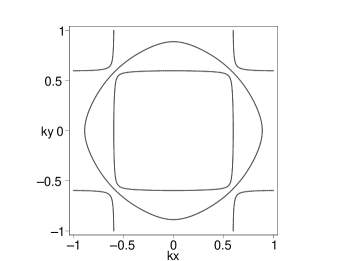
FIG. 1.: Fermi surface of Sr₂RuO₄ using the tight binding parameters in this paper ($k_{x}$ and $k_{y}$ are in units $\pi/a$ where $a$ is the lattice spacing). Moving out from the ${\bf k}=(0,0)$ point, first the $\beta$ sheet, then the $\gamma$ sheet, and finally the $\alpha$ sheet are crossed.

$f_{x}({\bf k})$	$f_{y}({\bf k})$	Fermi Surface	$\frac{H_{c2}^{100}}{H_{c2}^{110}}$	Impurity Dependent
$v_{x}$	$v_{y}$	$\gamma$	0.50	no
$(\cos k_{x}-\cos k_{y})v_{x}$	$-(\cos k_{x}-\cos k_{y})v_{y}$	$\gamma$	0.86	yes
$\sin k_{x}\sin k_{y}v_{y}$	$\sin k_{x}\sin k_{y}v_{x}$	$\gamma$	0.31	yes
$\sin k_{x}$	$\sin k_{y}$	$\gamma$	0.36	yes
$(\cos k_{x}-\cos k_{y})\sin k_{x}$	$(\cos k_{x}-\cos k_{y})\sin k_{y}$	$\gamma$	0.51	yes
$\sin^{2}k_{y}\sin k_{x}$	$\sin^{2}k_{x}\sin k_{y}$	$\gamma$	0.24	no
$v_{x}$	$v_{y}$	$\alpha$	2.0	no
$(\cos k_{x}-\cos k_{y})v_{x}$	$-(\cos k_{x}-\cos k_{y})v_{y}$	$\alpha$	3.9	yes
$\sin k_{x}\sin k_{y}v_{y}$	$\sin k_{x}\sin k_{y}v_{x}$	$\alpha$	1.2	yes
$v_{x}$	$v_{y}$	$\beta$	2.5	no
$(\cos k_{x}-\cos k_{y})v_{x}$	$-(\cos k_{x}-\cos k_{y})v_{y}$	$\beta$	5.23	yes
$\sin k_{x}\sin k_{y}v_{y}$	$\sin k_{x}\sin k_{y}v_{x}$	$\beta$	1.52	yes

TABLE I.: Upper critical field anisotropy for various gap functions for Sr₂RuO₄. Note that the normalization of the gap functions has not been included here. The column called Impurity Dependent states whether or not $H_{c2}^{100}/H_{c2}^{110}$ depends upon impurity scattering.

REFERENCES

• [1] D. J. van Harlingen, Rev. Mod. Phys. 67, 515 (1995).
• [2] L.P. Gor’kov, Sov. Sci. Rev., Sect. A 9, 1 (1987).
• [3] Y. Maeno, T.M. Rice, and M. Sigrist, Phys. Today 54, 42 (2001).
• [4] M. Rice, Nature , Nature 396, 627 (1998).
• [5] Y. Maeno et al., Nature 372, 532 (1994).
• [6] K. Ishida et al., Phys. Rev. B 56, 505 (1997).
• [7] A.P. Mackenzie et al., Phys. Rev. Lett. 80, 161 (1998).
• [8] K. Ishida et al., Nature (London) 96, 658 (1998).
• [9] T.M. Rice and M. Sigrist, J. Phys.: Condens. Matter 7, L643 (1995).
• [10] G. Baskaran, Physica B 223-224, 490 (1996).
• [11] M. Sigrist and K. Ueda, Rev. Mod. Phys. 63, 239 (1991).
• [12] G.M. Luke et al., Nature 394, 558 (1998).
• [13] P.G. Kealey et al., Phys. Rev. Lett. 84, 6094 (2000).
• [14] R. Jin, Y. Liu , Z.Q. Mao, and Y. Maeno, Europhys. Lett. 51, 341 (2000).
• [15] F. Laube et al., Phys. Rev. Lett. 84, 1595 (2000).
• [16] S. Nishizaki, Y. Maeno, and Z.Q. Mao, J. Low Temp. Phys. 117, 1581 (1999).
• [17] K. Ishida et al., Phys. Rev. Lett. 84, 5387 (2000).
• [18] I. Bonalde et al., Phys. Rev. Lett. 85, 4775 (2000).
• [19] Y. Hasegawa, K. Machida, and M. Ozaki, J. Phys. Soc. Jpn. 69, 336 (2000).
• [20] M.J. Graf and A.V. Balatsky, Phys. Rev. B 62, 9697 (2000).
• [21] H. Won and K. Maki, Europhys. Lett. 52, 427 (2000).
• [22] D.F. Agterberg, T.M. Rice, M. Sigrist, Phys. Rev. Lett. 78, 3374 (1997).
• [23] K. Miyake and O. Narikiyo, Phys. Rev. Lett. 83, 1423 (1999).
• [24] K. Kuroki et al., Phys. Rev. B 63, 060506(R) (2001).
• [25] M.E. Zhitomirsky and T.M. Rice, cond-mat/0102390.
• [26] Z.Q. Mao et al., Phys. Rev. Lett. 84, 991 (2000).
• [27] C. Petrovic et al., cond-mat/0011365.
• [28] R.H. Heffner et al., cond-mat/0102137.
• [29] D.F. Agterberg, Phys. Rev. B 58, 14 484 (1998).
• [30] M. Sigrist, J. Phys. Soc. Jpn. 69, 1290 (2000).
• [31] D.F. Agterberg, Phys. Rev. Lett. 80, 5184 (1998).
• [32] T. Oguchi Phys. Rev. B 51, 1385 (1995).
• [33] D.J. Singh, Phys. Rev. B 52, 1358 (1995).
• [34] I.I. Mazin and D.J. Singh, Phys. Rev. Lett. 79, 733 (1997).
• [35] T.M. Riseman et al., Nature 396, 242 (1998); and Nature 404, 629 (2000).
Refer to caption