Stripe Orientation in an Anisotropic $t$-$J$ Model

Early Hartree-Fock calculations [1] found evidence for domain-wall formation in doped 2D Hubbard and $t$-$J$ models. In these calculations the domain walls contained one hole per unit cell and separated $\pi$-phase shifted antiferromagnetic (AF) regions. Subsequent density-matrix-renormalization-group (DMRG) calculations [2] also found hole-domain walls separating $\pi$-phase shifted AF regions, but in these calculations the linear filling of the horizontal (or vertical) domain walls corresponded to one hole per two unit cells of the wall. In these calculations, domain-wall formation originates as a compromise in the inherent competition between the kinetic and exchange energies which arises when holes are added to a Mott antiferromagnetic insulator. In the parameter regime where horizontal or vertical stripes formed, these four-fold rotationally invarient models did not distinguish between the two orientations. Here we wish to discuss a possible electronic mechanism for stripe orientation.

We are motivated by the structural phase transition [3] of $La_{1.6-x}Nd_{0.4}Sr_{x}CuO_{4}$, in which the system goes from a low temperature orthorhombic (LTO) to a low temperature tetragonal (LTT) phase below $\sim 70K$. Here, as illustrated in Fig. 1a, in the LTT phase the $CuO_{6}$ octahedra tilt around an axis oriented along the planar $Cu$-$O$ bonds, say along the $y$-direction. As a consequence, oxygen atoms on the tilt axis remain in the plane, but in the perpendicular $x$-direction a staggered tilting pattern results with oxygen atoms $O_{a}$ and $O_{b}$ in Fig. 1a displaced above or below the $CuO_{2}$ plane, respectively. The $x$- and $y$-directions are therefore no longer equivalent in contrast to the LTO phase, where the tilt axis is rotated by 45 degrees, as shown in Fig. 1b.

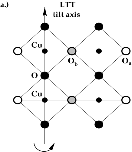
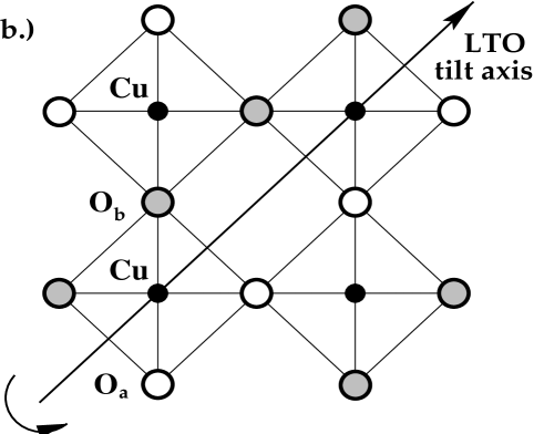
FIG. 1.: Planar view of the tilt pattern of the $CuO_{6}$ octahedra in the (a) LTT and (b) LTO phase. In (a) oxygen atoms along the vertical bonds remain in the $CuO_{2}$ plane while in the perpendicular direction they move below $(O_{b})$ or above $(O_{a})$ the plane in a staggered pattern, leading to a reduction of $t_{x}$ and $J_{x}$ relative to $t_{y}$ and $J_{y}$.

The electronic hopping integrals, and thus the antiferromagnetic superexchange, in the $CuO_{2}$ planes depends sensitively on the $Cu$-$O$-$Cu$ bond angle $\theta$. In the specific buckling pattern of the LTT phase, this bond angle is $\theta_{y}=\pi$ along the tilt axis direction, but is reduced by twice the octahedral tilt angle $\alpha$ in the perpendicular direction, i.e. $\theta_{x}=\pi-2\alpha$. This $x$-$y$ anisotropy for the electronic hopping and superexchange parameters may be conveniently translated into an anisotropic $t$-$J$ model Hamiltonian

$$H= - t_{x}\sum_{\langle i,i+x\rangle\sigma}\left(c^{\dagger}_{i+x\sigma}c_{i\sigma}+h.c.\right)$$ (1)

$$+ J_{x}\sum_{\langle i,i+x\rangle}\left({\bf S}_{i+x}\cdot{\bf S}_{i}-\frac{n_{i+x}n_{i}}{4}\right)$$ (2)

$$- t_{y}\sum_{\langle i,i+y\rangle\sigma}\left(c^{\dagger}_{i+y\sigma}c_{i\sigma}+h.c.\right)$$ (3)

$$+ J_{y}\sum_{\langle i,i+y\rangle}\left({\bf S}_{i+y}\cdot{\bf S}_{i}-\frac{n_{i+y}n_{i}}{4}\right)\ .$$ (4)

Here, $\langle i,i+x\rangle$ and $\langle i,i+y\rangle$ denote nearest-neighbor sites along the $x$- and $y$-directions on a square lattice, respectively, and doubly-occupied sites are explicitly excluded from the Hilbert space.

The magnitude of the anisotropies is easily estimated for typical tilt angles of $4^{\circ}$–$5^{\circ}$ in $La_{1.6-x}Nd_{0.4}Sr_{x}CuO_{4}$ with $x$ near 1/8 [3]. When the tilt axis of the LTT phase is vertical, as shown in Fig. 1a, we have

$$\frac{t_{x}}{t_{y}}\cong|\cos(\pi-2\alpha)|\qquad{\rm and}\qquad\frac{J_{x}}{J_{y}}\cong\cos^{2}(\pi-2\alpha)$$ (5)

It follows that for a tilt angle of order $4^{\circ}$–$5^{\circ}$, $\Delta t/t\sim 1.$–1.5% and $\Delta J/J\sim 2.$–3.%. We note that the direction with the larger exchange coupling is naturally also the direction with the larger hopping amplitude. Choosing $t=500$meV and with the exchange coupling constant $J=1500K$ of undoped $La_{2}CuO_{4}$ these estimates give $\Delta t=|t_{x}-t_{y}|\sim 60K$ and $\Delta J=|J_{x}-J_{y}|\sim 40K$. This rough estimate for the exchange anisotropy agrees with results from quantum chemistry calculations [4].

Given this model Hamiltonian, with $J_{y}>J_{x}$ and $t_{y}>t_{x}$, one may ask in which direction stripes are expected to form. Since $J_{y}>J_{x}$, the exchange energy is optimized by orienting the domain walls along the $y$-axis so as to minimize the number of broken exchange bonds in the direction with the stronger superexchange. Now, one might be tempted to argue that since $t_{y}>t_{x}$, this also lowers the kinetic energy of the system. However, transverse motion of the domain walls is also known to be important [1, 5, 7], so that an anisotropy in the hopping with $t_{y}>t_{x}$ can favor a horizonal orientation of the stripes. Because $\Delta J$ and $\Delta t$ are comparable in magnitude, we analyze the results of a DMRG calculation to obtain further insight in this point.

We have used DMRG techniques to study a $9\times 8$ lattice with periodic boundary conditions in the 8-site $y$-direction and open boundary conditions in the 9-site $x$-direction. Fig.2a shows a domain which forms when 4 holes are added for an isotropic Hamiltonian with $J/t=0.35$. The boundary conditions cause the domain to form around the middle of this 8-leg cylinder. According to the Hellman-Feynman theorem,

$$\frac{\partial\langle H\rangle}{\partial J_{x}}=\sum_{\langle ij\rangle\atop x{\rm-bonds}}\left\langle\vec{S}_{i}\cdot\vec{S}_{j}-\frac{n_{i}n_{j}}{4}\right\rangle$$ (6)

Therefore, by calculating the change

$$\Delta\left\langle\vec{S}_{i}\cdot\vec{S}_{j}-\frac{n_{i}n_{j}}{4}\right\rangle = \left\langle\vec{S}_{i}\cdot\vec{S}_{j}-\frac{n_{i}n_{j}}{4}\right\rangle_{4}$$ (7)

$$- \left\langle\vec{S}_{i}\cdot\vec{S}_{j}-\frac{n_{i}n_{j}}{4}\right\rangle_{o}$$ (8)

between the expectation value in the 4-hole ground state and the undoped ground state for the isotropic case with a given value of $J/t$, we can determine the variation of the domain wall energy with respect to small changes in $J_{x}$ near $J$. The local change for the individual $x$-bonds, eq. (8), which contribute to $\partial\langle H\rangle/\partial J_{x}$ are shown on the horizontal $x$-bonds in Fig. 2b for $J/t=0.35$. Note that these contributions decrease as one moves away from the domain wall and we find that

$$\frac{1}{4}\ \frac{\partial}{\partial J_{x}}\ \left(\langle H\rangle_{4}-\langle H\rangle_{o}\right) = -\frac{1}{4}\ \sum_{\langle ij\rangle\atop x{\rm-bonds}}\Delta\left\langle\vec{S}_{i}\cdot\vec{S}_{j}-\frac{n_{i}n_{j}}{4}\right\rangle$$ (9)

$$= 1.91/{\rm hole}\ .$$ (10)

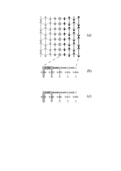
FIG. 2.: (a) A $9\times 8$ lattice with $J/t=0.35$ and 4 holes which form a site-centered domain wall. This lattice has periodic boundary conditions in the $y$-direction and open ends in the $x$-direction where a weak, $\pi$-phase shifted staggered magnetic field $h=\pm 0.1t$, is applied at the open ends. The diameter of the circles indicate the hole density and the length of the spins, the spin magnitude. The length of the arrows on the left and right sides corresponds to $\langle S_{z}\rangle=0.37$. The hole density, which is proportional to the diameter of the gray circles, is $\langle n_{h}\rangle=0.155$ along the center of the stripe. (b) The change in $\langle(\vec{S}_{i}\cdot\vec{S}_{j}-\frac{1}{4}n_{i}n_{j})\rangle$ between the 4-hole ground state with the domain wall and the undoped Heisenberg lattice. In the undoped case the weak applied staggered end-field was periodic. The value 0.194 corresponds to the axis of the domain wall, and the values are symmetric about this axis. (c) The kinetic energy $-\sum_{s}\langle(c^{\dagger}_{is}c_{js}+h.c.)\rangle$ in units of $t$ of the 4-hole system.

In a similar manner we find that the variation of the domain wall energy with the exchange energy $J_{y}$ parallel to the wall gives

$$\frac{1}{4}\ \frac{\partial}{\partial J_{y}}\,\left(\langle H\rangle_{4}-\langle H\rangle_{o}\right) = -\frac{1}{4}\ \sum_{\langle ij\rangle\atop y{\rm-bonds}}\Delta\left\langle\vec{S}_{i}\cdot\vec{S}_{j}-\frac{n_{i}n_{j}}{4}\right\rangle$$ (11)

$$= 1.20/{\rm hole}\ .$$ (12)

Continuing with the kinetic energy terms,

$$\frac{1}{4}\ \frac{\partial}{\partial t_{x}}\ \langle H\rangle_{4} = -\frac{1}{4}\sum_{\langle ij\rangle s\atop x{\rm-bonds}}\left\langle c^{\dagger}_{is}c_{js}+c^{\dagger}_{js}c_{is}\right\rangle$$ (13)

$$= -1.43/{\rm hole}$$ (14)

and

$$\frac{1}{4}\ \frac{\partial}{\partial t_{y}}\ \langle H\rangle_{4} = -\frac{1}{4}\sum_{\langle ij\rangle s\atop y{\rm-bonds}}\left\langle c^{\dagger}_{is}c_{js}+c^{\dagger}_{js}c_{is}\right\rangle$$ (15)

$$= -1.43/{\rm hole}\ .$$ (16)

The local kinetic energy of the 4-hole systems associated with the domain wall are listed in Fig. 2c.

Now, if the tilt axis of the LTT structure runs along the $y$-axis so that it is parallel to the domain wall, then $J_{y}=J$, $J_{x}=J-\Delta J$, $t_{y}=t$, and $t_{x}=t-\Delta t$. In this case, the shift in energy per hole of the domain wall due to the small anisotropy is

$$\Delta E_{\|}=-1.9\Delta J+1.41\Delta t\ .$$ (17)

Alternatively, if the LTT tilt axis runs along the $x$-axis, perpendicular to the domain wall, the shift in energy per hole is

$$\Delta E_{\perp}=-1.20\Delta J+1.43\Delta t\ .$$ (18)

Therefore, if the domain wall is oriented parallel to the LTT tilt axis, there is a net energy reduction (relative to an orientation perpendicular to the tilt axes) of

$$\Delta E=0.7\Delta J-0.02\Delta t\simeq 25K/{\rm hole}\ .$$ (19)

For a section of domain wall containing 4 holes, this would be 100K. The extensive nature of this energy favors alignment of the domain wall with the LTT tilt axis.

Thus we conclude that the $\Delta J$ anisotropy dominates and favors orienting the stripes along the direction of the tilt axis of the LTT phase. This is the same orientation as suggested from the “structural corrugation” driven orientation mechanism originally set forth by Tranquada et. al. [6]. Here, we have simply looked at a particular model in which the corrugation manifests itself by giving rise to an anisotropic $t$-$J$ model.

REFERENCES

[1] J. Zaanen and O. Gunnarsson, Phys. Rev. B40,
7391 (1989); D. Poilblanc and T.M. Rice, Phys. Rev. B39, 9749
(1989).
[2] S.R. White and D.J. Scalapino, Phys. Rev. Lett.80, 1272 (1998); ibid.81, 3227 (1998).
[3] B. Büchner et al., Phys. Rev. Lett.73, 1841
(1994); H.-H. Klauß et al., in preparation.
[4] R.L. Martin, private communication.
[5] B. Normand and A.P. Kampf, preprint cond- mat/0102201.