Fluctuation-Dominated Phase Ordering Driven by Stochastically Evolving Surfaces

Abstract

We study a new kind of phase ordering phenomenon in coarse-grained depth models of the hill-valley profile of fluctuating surfaces with zero overall tilt, and for hard-core particles sliding on such surfaces under gravity. We find that several such systems approach an ordered state with large scale fluctuations which make them qualitatively different from conventional phase ordered states. We consider surfaces in the Edwards-Wilkinson (EW), Kardar-Parisi-Zhang (KPZ) and Golubovic-Bruinsma-Das Sarma-Tamborenea (GBDT) universality classes. For EW and KPZ surfaces, coarse-grained depth models of the surface profile exhibit coarsening to an ordered steady state in which the order parameter has a broad distribution even in the thermodynamic limit, the distribution of particle cluster sizes decays as a power-law (with an exponent $\theta$), and the 2-point spatial correlation function has a cusp (with an exponent $\alpha=1/2$) at small values of the argument. The latter feature indicates a deviation from the Porod law which holds customarily, in coarsening with scalar order parameters. We present several numerical and exact analytical results for the coarsening process and the steady state. For linear surface models with dynamical exponent $z$, we show that $\alpha=(z-1)/2$ for $z<3$, $\alpha=1$ for $z>3$, and there are logarithmic corrections for $z=3$, implying $\alpha=1/2$ for the EW surface and $1$ for the GBDT surface. Within the independent interval approximation we show that $\alpha+\theta=2$. We also study the dynamics of hard-core particles sliding locally downwards on these fluctuating one-dimensional surfaces and find that the surface fluctuations lead to large-scale clustering of the particles. We find a surface-fluctuation driven coarsening of initially randomly arranged particles; the coarsening length scale grows as $\sim t^{1/z}$. The scaled density-density correlation function of the sliding particles shows a cusp with exponent $\alpha\simeq 0.5$, and $0.25$ for the EW and KPZ surfaces. The particles on the GBDT surface show conventional coarsening (Porod) behavior with $\alpha\simeq 1$.

PACS numbers: 05.70.Ln, 05.40.-a, 02.50.-r, 64.75.+g

I Introduction

Phase ordering dynamics describes the way in which domains of an ordered state develop when an initially disordered system is placed in an environment which promotes ordering. For instance, when a simple ferromagnet or alloy is quenched rapidly from very high to very low temperatures $T$, domains of equilibrium low-$T$ ordered phases form and grow to macroscopic sizes. A quantitative description of the ordering process is provided by the time development of the two-point correlation function; asymptotically, it is a function only of the separation scaled by a length which increases with time, typically as a power law [2].

New phenomena and effects can arise when we deal with phase ordering in systems which are approaching nonequilibrium steady states. In this paper, we study a coupled-field nonequilibrium system in which one field evolves autonomously and influences the dynamics of the other. The system shows phase ordering of a new sort, whose principal characteristic is that fluctuations are very strong and do not damp down in the thermodynamic limit — hence the term fluctuation-dominated phase ordering (FDPO).

In usual phase ordering systems such as ferromagnetic Ising model, if one considers a finite system and waits for infinite time, then the system reaches a state with magnetization per site very close to the two possible values of the spontaneous magnetization, $m_{s}$ or $-m_{s}$, with very infrequent transitions between the two. This is reflected in a probability distribution for the order parameter which is sharply peaked at these two values, with the width of the peaks approaching zero in the thermodynamic limit (Fig. 1(a)). By contrast, in the FDPO steady state, the system continually shows strong fluctuations in time without, however, losing macroscopic order. Accordingly, the order parameter shows strong variations in time, reflected eventually in a probability distribution which remains broad even in the thermodynamic limit (Fig. 1(b)).

The physical system we study consists of an independently stochastically fluctuating surface of zero average slope, on which reside particles which tend to slide downwards guided by the local slopes of the surface. Somewhat surprisingly, a state with uniform particle density is unstable towards large scale clustering under the action of surface fluctuations. Eventually it is driven to a phase-ordered state with macroscopic inhomogeneities of the density, of the FDPO sort. Besides exhibiting a broad order parameter distribution, this state shows unusual scaling of two-point correlation functions and cluster distributions. It turns out that much of the physics of this type of ordering is also captured by a simpler model involving a coarse-grained characterization of the surface alone, and we study this as well. A brief account of some of our results has appeared in [3].

FIG. 1.: Schematic depiction of $Prob(m)$ against $m$ in steady state for $(a)$ a normal phase ordering system such as a ferromagnet at low temperature $(b)$ a system showing FDPO.

In the remainder of the introduction, we first discuss the characteristics of FDPO vis a vis normal phase-ordered states. We then discuss, in a qualitative way, the occurrence of FDPO in the surface-driven models under study. The layout of the rest of the paper is as follows. In Section II, we define and study the coarsening and steady states of three different coarse-grained depth models of the fluctuating surfaces. In Section III, we demonstrate the existence of a power-law in the cluster size distribution, and show how it can give rise to FDPO. In Section IV, we discuss ordering of sliding particles on fluctuating surfaces. In Section V, we explore the robustness of FDPO with respect to changes in various rates defining the nonequilibrium process. Finally, in Section VI we summarize our principal results, and discuss the possible occurrence of FDPO in models of other physical systems.

A Ordered States in Equilibrium Systems

With the aim of bringing out the features of fluctuation dominated phase ordering (FDPO) in nonequilibrium systems, let us recall some familiar facts about phase ordered states in equilibrium statistical systems. We first discuss different characterizations of spontaneous ordering, following the paper of Griffiths [4] on the magnetization of idealized ferromagnets. We follow this with a discussion of fluctuations about the ordered state.

1 Definitions of Spontaneous Order

(a) In the absence of a conservation law, the magnetization $m$ is an indicator of the ordering:

$$m={{1\over L^{d}}{\sum_{n}}s_{n}}$$ (1)

where $L$ is the linear size, $d$ is the dimension and $s_{n}$ is spin at site $n$. In the thermodynamic limit, the thermal average of the absolute value

$$m_{1}={Lim_{L\rightarrow\infty}}\langle|m|\rangle~{}~{}({\rm nonconserved})$$ (2)

with Boltzmann-Gibbs weights for configurations provides an unequivocal measure of the order. This is because in the low-temperature ordered phase, the probability $Prob(m)$ of occurrence of magnetization $m$ is peaked at $+m_{s}$ and $-m_{s}$; the peak widths approach zero in the thermodynamic limit $L\rightarrow\infty$, so that the average value $m_{1}$ coincides with the peak value $m_{s}$ (Fig. 1$(a)$).

For the conserved order parameter case, the value of the magnetization is a constant and is same in both the disordered and ordered phase. One therefore needs a quantity that is sensitive to the difference between order and disorder. The simplest such quantity is the lowest nonzero Fourier mode of the density [5]

$$|Q|={1\over L}{|{\sum_{n}}e^{2\pi in/L}{(1+S_{n})\over 2}|}$$ (3)

where $S_{n}$ denotes the average magnetization in the $(d-1)$-dimensional plane $n$ oriented perpendicular to the $x$ direction. The modulus in Eq. 3 above leads to the same value for all states which can be reached from each other by a translational shift. In the low-$T$ ordered phase, $Prob(Q)$ is expected to be a sharply peaked function, with peak widths vanishing in the thermodynamic limit. Then the mean value $Q_{1}$ defined by

$$Q_{1}={Lim_{L\rightarrow\infty}}\langle|Q|\rangle~{}~{}({\rm conserved})$$ (4)

serves as an order parameter. A disordered state corresponds to $Q_{1}=0$, while a perfectly ordered state with $m=1$ in half of the system and $m=-1$ in the other half corresponds to $Q_{1}={1/\pi}\simeq 0.318.$

(b) Another characterization of the order is obtained from the asymptotic value of the 2-point spatial correlation function $C(r)=\langle s_{o}s_{o+r}\rangle$. At large separations $r$, $C(r)$ is expected to decouple:

$${Lim_{r\rightarrow\infty}}{Lim_{L\rightarrow\infty}}\langle s_{o}s_{o+r}\rangle=\langle s_{o}\rangle\langle s_{o+r}\rangle=m_{c}^{2}.$$ (5)

A finite value of $m_{c}$ indicates that the system has long-range order. A value $m_{c}=1$ would indicate a perfectly ordered pure phase without any droplets of the other species (like the $T=0$ state of an Ising ferromagnet), while $m_{c}\neq 1$ would indicate that the phase has an admixture of droplets of the other species (like the state of an Ising ferromagnet for $0<T<T_{c}$).

In a finite system, $C$ is a function only of the scaled variable $r/L$ in the asymptotic scaling limit $r\rightarrow\infty,L\rightarrow\infty$ (see also (d) below). An operational way to find the value of $m_{c}$ is then to read off the intercept ($r/L\rightarrow 0$) in a plot of $C$ versus $r/L$; it gives $m_{c}^{2}$ in the $L\rightarrow\infty$ limit.

In equilibrium systems of the type discussed above, $m_{1}$ (defined in Eq. 2) and $m_{c}$ coincide.

2 Characteristics of Fluctuations

(c) With a conserved scalar order parameter, the low-$T$ state is phase-separated, with each phase occupying a macroscopically large region, and separated from the other phase by an interface of width $W$. The interfacial region is quite distinct from either phase, and on the scale of system size, it is structureless and sharp.

(d) Customarily in phase-ordered steady states, the spatial correlation function $C(r)$ has a scaling form in $|r/L|$, for $\xi<<r<<L$ where $L$ is the size of the system. In the limit $r\rightarrow\infty,L\rightarrow\infty,|r/L|\rightarrow 0$, $C(r)$ follows the form [2]

$$C(r)\approx m_{c}^{2}(1-2|r/L|)~{}~{}~{}~{}(|r/L|\rightarrow 0)$$ (6)

The origin of the linear fall in Eq. 6 is easy to understand in systems where phases are separated by sharp boundaries on the scale of the system size, as in (c) above: a spatial averaging of $s_{o}s_{o+r}$ produces $+m_{c}^{2}$ with probability $(1-|r/L|)$ (within a phase) and $-m_{c}^{2}$ with probability $|r/L|$ (across phases). The linear drop with $|r/L|$ implies that the structure factor $S(k)$, which is the Fourier transform of $C(r)$, is given, for large wave-vectors $(kL>>1$), by:

$${S(k)\over L^{d}}\sim{1\over{(kL)}^{d+1}}.$$ (7)

This form of the decay of the structure factor for scalar order parameters is known as the Porod law.

It is worth remarking that the forms Eqs. 6 and 7 also describe the behaviour of the two-point correlation function in an infinite system undergoing phase ordering starting from an initially disordered state. In such a case, $L$ denotes the coarsening time-dependent length scale which is the characteristic size of an ordered domain.

(e) For usual phase-ordered systems, spatial fluctuations are negligible in the limit of the system size going to infinity. Hence the averages of 1-point and 2-point functions over an ensemble of configurations are well represented by a spatial average for a single configuration in a large system.

B Fluctuation-Dominated Ordering

The phase ordering of interest in this paper occurs in certain types of nonequilibrium systems, and the resulting steady state differs qualitatively from the ordered state of equilibrium systems and other types of nonequilibrium systems considered earlier [6]. The primary difference lies in the effects of fluctuations. Customarily, fluctuations lead to large variations of the order parameter which scale sublinearly with the volume, and so are negligible in the thermodynamic limit. Fluctuation effects are much stronger here, and lead to variations of the order parameter in time, without, however, losing the fact of ordering. Below we discuss how the properties (a)-(e) discussed above are modified.

(a) Nonzero values of the averages $M_{1}$ and $Q_{1}$ (Eqs. 2 and 4) continue to indicate the existence of order, but no longer provide an unequivocal measure of the order parameter. This is because the probability distributions $Prob(m)$ and $Prob(Q)$ remain broad even in the limit $L\rightarrow\infty$ (as shown schematically in Fig 1$(b)$).

(b) The measure $|m_{c}|$ of long-range order is nonzero, and its value can be found from the intercept $C(|r/L|\rightarrow 0)$. However, the value of $m_{c}$ is, in general, quite different from $m_{1}$.

(c) As with usual ordered states, the regions of pure phases are of the order of system size $L$. But in contrast to the usual situation, there need not be a well-defined interfacial region, distinct from either phase. Rather, the region between the two largest phase stretches is typically a finite fraction of the system size, and has a lot of structure; this region itself contains stretches of pure phases separated by further such regions, and the pattern repeats. Representative spin configurations $\{s_{i}\}$ for the two cases are depicted schematically in Fig. 2. This nested structure is consistent with a power-law distribution of cluster sizes, and thus of a critical state. The crucial extra feature of the FDPO state is that the largest clusters occupy a finite fraction of the total volume, and it is this which leads to a finite value of $m_{c}$ as in (b) above. Representative spin configurations $\{s_{i}\}$ for the two cases are depicted schematically in Fig. 2.

FIG. 2.: Schematic depiction of a linear and a cuspy decay of $C(r)$ as a function of $r/L$, characteristic of normal phase ordering and FDPO respectively. Typical configurations corresponding to the two cases are also shown, with 1 and $-1$ denoting the values of $s_{i}$.

(d) The ensemble-averaged spatial correlation function $C(r)$ continues to show a scaling form in $|r/L|$. However, in contrast to Eq. 7 it exhibits a cusp (Fig. 2) at small values of $|r/L|$:

$$C(r)\approx m_{c}^{2}(1-b{|{r\over L}|}^{\alpha}).$$ (8)

This implies that the scaled structure factor varies as

$${S(k)\over L^{d}}\sim{1\over{(kL)}^{d+\alpha}}$$ (9)

with $\alpha<1$. This represents a marked deviation from the Porod law (Eq. 7). We will demonstrate in some cases that this deviation is related to the power-law distribution of clusters in the interfacial region separating the domains of pure phases, as discussed in (c) above.

(e) The spatial average of 1-point functions ($m$ or $Q$) and the 2-point function $C$ as a function of $|r/L|$ in a single configuration of a large system typically do not represent the answers obtained by averaging over an ensemble of configurations. This reflects the occurrence of macroscopic fluctuations.

C Fluctuating Surfaces and Sliding Particles

Having described the general nature of fluctuation-dominated phase ordering, we now discuss the model systems that we have studied and which show FDPO. We consider physical processes defined on a fluctuating surface with zero average slope. The surface is assumed to have no overhangs, and so is characterized by a single-valued local height variable $h(x,t)$ at position $x$ at time $t$ as shown in Fig. 3. The evolution of the height profile is taken to be governed by a stochastic equation. The height-height correlation function has a scaling form [7] for large separations of space and time:

$$\langle[h(x,t)-h(x^{\prime},t^{\prime})]^{2}\rangle\sim|x-x^{\prime}|^{2\chi}f({|t-t^{\prime}|\over|x-x^{\prime}|^{z}}).$$ (10)

Here $f$ is a scaling function, and $\chi$ and $z$ are the roughness and dynamical exponents, respectively. A common value of these exponents and scaling function for several different models of surface fluctuations indicate a common universality class for such models. In this paper we will study one-dimensional surfaces belonging to three such universality classes of surface growth. Similar studies of two-dimensional surfaces [8] show that similar fluctuation-dominated phase-ordered states arise in these cases as well.

FIG. 3.: Schematic depiction of a surface with height $h(x,t)$ and the coarse-grained depth function $s(x,t)$.

Before turning to the physical model of particles sliding on such fluctuating surfaces, we address the notion of phase ordering in coarse-grained depth models associated with these surface fluctuations. In Fig. 3 we show the function $s(x,t)$ which take values $+1$, $-1$ and $0$ depending on whether the height is below, above or at the same level as some reference height $\langle h\rangle$. Explicitly, we have $s(x,t)=-sgn(h(x,t)-\langle h\rangle)$. Different definitions of $\langle h\rangle$ define variants of the model; these are studied in Section II.

Starting from initially flat surfaces, we study the coarsening of of up-spin or down spin phases, which arise from the evolution of surface profiles. With the passage of time, the surface gets rougher up to some length scale ${\cal L}(t)$. The profile has hills and valleys, the base lengths of which are of the order of ${\cal L}(t)$, implying domains of like-valued $s$ whose size is of the same order. Once the steady state is reached, there are landscape arrangements of the order of the system size $L$ which occur on a time scale $L^{z}$. However, these landscape fluctuations do not destroy long-range order, but cause large fluctuations in its value.

Now let us turn to the problem of hard-core particles sliding locally downwards under gravity on these fluctuating surfaces. Figure 4 depicts the evolution of particles falling to the valley bottoms under gravity. When a local valley forms in a region (Fig. 3(a) $\rightarrow$ Fig. 3(b)), particles in that region tend to fall in and cluster together. The point is that particles stay together even when there is a small reverse fluctuation (valley $\rightarrow$ hill as in Fig. 4(b) $\rightarrow$ (c)); declustering occurs only if there is a rearrangement on length scales larger than the size of the valley. The combination of random surface fluctuations and the external force due to gravity drive the system towards large-scale clustering. Results of our numerical studies show that in the coarsening regime, the typical scale of ordering in the particle-hole system is comparable to the length scale over which surface rearrangements take place. Further, the steady state of the particle system exhibits uncommonly large fluctuations, reflecting the existence of similar fluctuations in the underlying coarse-grained depth models of the hill-valley profile. Similar effects are seen in 1-point and 2-point correlation functions.

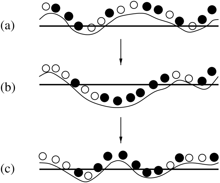
FIG. 4.: Depicting clustering of particles ($\bullet$) in a section of the fluctuating surface. A surface fluctuation such as $(a)\rightarrow(b)$ causes the particles to roll into a valley. They remain clustered even after a local reverse surface fluctuation $(b)\rightarrow(c)$ occurs.

II FDPO in coarse-grained depth (CD) models of surfaces

A Surface evolution

The dynamics of surface fluctuations can be modelled by Langevin-type equations for the height field $h(x,t)$. The evolution equations for the one-dimensional Edwards-Wilkinson (EW) [9], Kardar-Parisi-Zhang (KPZ) [10], and Golubovic-Bruinsma-Das Sarma-Tamborenea (GBDT) [11] surface fluctuations are respectively

$$EW:~{}{{\partial h}\over{\partial t}} = \nu_{1}{{\partial^{2}h}\over{\partial x^{2}}}+\eta_{1}(x,t)$$ (11)

$$KPZ:~{}{{\partial h}\over{\partial t}} = \nu_{1}{{\partial^{2}h}\over{\partial x^{2}}}+\lambda({{\partial h}\over{\partial x}})^{2}+\eta_{1}(x,t)$$ (12)

$$GBDT:~{}{{\partial h}\over{\partial t}} = -K{{\partial^{4}h}\over{\partial x^{4}}}+\eta_{1}(x,t)$$ (13)

where  $\eta_{1}(x,t)$  is  a  white  noise  with  $\langle\eta_{1}\rangle=0$  and $\langle\eta_{1}(x^{\prime},t^{\prime})\eta_{1}(x,t)\rangle=\Gamma{\delta(x^{\prime}-x)}{\delta(t^{\prime}-t)}$, and $\nu_{1}$, $\lambda$ and $K$ are constants.

In one dimension, the EW and KPZ models can be simulated using lattice gas models whose large-distance large-time scaling properties coincide with those of the corresponding continuum theories. The lattice gas is composed of $\pm 1$-valued variables $\{\tau_{i-{1\over 2}}\}$ on a $1-d$ lattice with periodic boundary conditions, where the ${\tau}$ spins occupy the links between sites. The values $\tau_{i-{1\over 2}}=+1$ or $-1$ represent the local slopes of the surface (denoted by $/$ or $\backslash$, respectively). The dynamics of the interface is that of the single-step model [12], with stochastic corner flips involving exchange of adjacent $\tau$’s; thus, $/\backslash\rightarrow\backslash/$ with rate $p_{1}$, while $\backslash/\rightarrow/\backslash$ with rate $q_{1}$. For symmetric surface fluctuations ($p_{1}=q_{1}$), the behavior at large length and time scale is described by the continuum EW model. For $p_{1}\neq q_{1}$, the surface evolution belongs to the KPZ class. Corresponding to the configuration $\{\tau_{j-{1\over 2}}\}$ we have the height profile $\{h_{i}\}$ with $h_{i}={\sum_{1{\leq}j{\leq}i}}\tau_{j-{1\over 2}}$.

For simulating a surface fluctuating via a GBDT process, we used a solid-on-solid model with depositing particles piling up on top of each other. The height $h_{i}$ at site $i$ is the height of the pile of particles at that site. During each micro-step a particle is deposited randomly on a site $i$. If the new height $h_{i}$ at $i$, is greater than $h_{i-1}$ and $h_{i+1}$, then with equal probability ($=1/3$) three things are attempted — the deposited particle can remain at site $i$, or can move to the neighboring sites $i-1$ or $i+1$. It actually completes the left or right move only if there is an increase in the coordination-ordination number of the particles [7].

B Definitions of the CD models

Let us imagine a process of coarse-graining which eliminates fine fluctuations of the height profile, and replaces the height field $h_{i}$ at site $i$ by a variable $s_{i}$ which is +1, -1 or 0 depending on whether the surface profile at site $i$ is below, above or exactly coincident with a certain reference level, which is the same at all $i$. The aim is to have a coarse-grained construction of locations of large valleys and hills. Our procedure depends on the choice of the reference level, and we have explored three choices (the CD1, CD2 and CD3 models) which are discussed below.

In model CD1, the reference level is set by the initial condition, which corresponds to an initially flat interface: $h(x,t=0)=0$. The coarse-grained depth function is then

$$s(x,t)=-sgn[h(x,t)].$$ (14)

With the passage of time, the surface becomes rougher, so that $h(x,t)$ develops hills and valleys with respect to the $0$ level. As the base lengths of the hills and valleys grow in size, there is a growth of the domains of the variable $s(x,t)$. We are able to characterize the coarsening behaviour of this model analytically in some cases.

In a finite system, at long enough times the surface moves arbitrarily far away from its initial location. Thus the steady state of the CD1 model is trivial — all $s_{i}$ are 1, or all are -1, with probability one. This clearly happens because the reference level in the CD1 model is fixed in space. This leads us to examine models (CD2 and CD3) where the reference level moves along with the surface, so that we may expect nontrivial steady state properties.

In model CD2, the coarse-grained depth function

$$s_{i}=-sgn[h_{i}]$$ (15)

where $h_{i}={\sum_{1{\leq}j{\leq}i}}\tau_{j-{1\over 2}}$ as defined in the earlier section. Note that at all times $t$, the origin is pinned so that $h_{i=0}=0$. The height function of the continuum version of the CD2 model is related to that of CD1 as: $h_{j}^{CD2}(t)=h_{j}^{CD1}(t)-h_{0}^{CD1}(t)$. The function $s_{i}$ is $+1$, $-1$ or $0$ accordingly as the height $h_{i}$ at site $i$ is below, above or at the zero level. A stretch of like $s_{i}$’s $=+1$ represents a valley with respect to the zero level. The time evolution of the CD2 model variables $\{s_{i}\}$ is induced by the underlying dynamics of the bond variables $\{\tau_{i-{1\over 2}}\}$ defined in the previous subsection. This model was studied by us in [3].

Finally model CD3, is defined as follows: $h_{i}$ is constructed from $\tau$’s exactly as described for the CD2 model, but then one defines

$$s_{i}=-sgn[h_{i}-\langle h(t)\rangle]$$ (16)

where $\langle h(t)\rangle=(1/L)\sum_{i=1}^{L}h_{i}(t)$ is the instantaneous average height which fluctuates with time. This definition was used earlier by Kim et al [13] who were studying domain growth in an evolving KPZ surface.

Each of the CD models defined above has its own merits and limitations. We will see below that the CD1 model proves to be analytically tractable (for Gaussian surface fluctuations) in the coarsening regime, while for the CD2 model several exact results can be derived in the steady state. Of the three models, the CD3 model most resembles the model of sliding hard-core particles on the surface that is studied in Section IV below.

C Coarsening in the CD models

1 Analytical results for the CD1 model

In this section, our primary focus is on coarsening properties of a class of CD1 models. To this end, we will focus on the equal time correlation function

$$C(x,t)=\langle\sigma(0,t)\sigma(x,t)\rangle=\langle sgn[h(0,t)]sgn[h(x,t)]\rangle.$$ (17)

We consider only linear interfaces evolving from a flat initial condition $h(x,0)=0$ according to the Langevin equation,

$${{\partial h}\over{\partial t}}=-{\left(-\nabla^{2}\right)}^{z/2}h+\eta,$$ (18)

where $\eta(x,t)$ is a Gaussian white noise with $\langle\eta(x,t)\rangle=0$ and $\langle\eta(x,t)\eta(x^{\prime},t^{\prime})\rangle=\delta(x-x^{\prime})\delta(t-t^{\prime})$. The dyanmic exponent $z$ specifies the relaxation mechanism. For example, $z=2$ corresponds to Edwards-Wilkinson (EW) interface and $z=4$ corresponds to Golubovic-Bruinsma-Das Sarma-Tamborenea (GBDT) interface. Since $\eta(x,t)$ is a Gaussian noise and the evolution equation (18) is linear, the height field $h(x,t)$ is a Gaussian process. For Gaussian processes, it is straightforward to evaluate the correlation function in Eq. (17) exactly and one finds,

$$C(x,t)={2\over{\pi}}{\sin}^{-1}\left[H(x,t)\right],$$ (19)

where $H(x,t)$ is given by,

$$H(x,t)={{\langle h(0,t)h(x,t)\rangle}\over{{\sqrt{\langle h^{2}(0,t)\rangle\langle h^{2}(x,t)\rangle}}}}.$$ (20)

Now the normalized height correlation function $H(x,t)$ can be easily computed for linear interfaces evolving via Eq. (18) by taking the Fourier transform of Eq. (18). From Eq. (18), assuming flat initial condition, the Fourier transform, $\langle h(k,t)h(-k,t)\rangle$ is given exactly by,

$$\langle h(k,t)h(-k,t)\rangle={(1-e^{-2|k|^{z}t})\over{2|k|^{z}}}.$$ (21)

Inverting this Fourier transform we get,

$$H(x,t)={(z-1)\over{2^{1-{1\over z}}\Gamma({1\over{z}})}}F\left({x\over{t^{1\over{z}}}}\right),$$ (22)

where the scaling function $F(y)$ is given by,

$$F(y)=\int_{0}^{\infty}{{1-e^{-2u^{z}}}\over{u^{z}}}\cos(yu)du.$$ (23)

Using this exact expression of $H(x,t)$ in Eq. (19), we get the exact correlation function for arbitrary linear interface model parametrized by the dynamic exponent $z$. It is also evident that $C(x,t)$ is a single function of the scaled distance, $y=xt^{-1/z}$.

The small distance behavior of the scaling function can be easily derived from the small argument asymptotics of the integral in Eq. (23). Let us first consider the EW interface with $z=2$. In this case the integral in Eq. (23) can be done (by putting a factor $w$ in the exponential, i.e., writing $e^{-2wz^{2}}$ and then differentiating with respect to $w$ and then integrating back with respect to $w$ upto $w=1$) and we get,

$$H(x,t)={1\over{2}}\int_{0}^{1}dww^{-1/2}e^{-x^{2}/{8wt}}.$$ (24)

A change of variable, $x^{2}/{8wt}=y$ gives a more compact expression,

$$H(x,t)={|x|\over{4\sqrt{2t}}}\int_{x^{2}/{8t}}^{\infty}e^{-y}y^{-3/2}dy.$$ (25)

Integration by parts yields the desired short distance behaviour,

$$H(x,t)=1-{\sqrt{\pi\over{8t}}}\,|x|+\ldots$$ (26)

Putting this back in Eq. (10) and expanding the arcsine, we get,

$$C(x,t)=1-{\left({2\over{\pi}}\right)}^{3/4}{|xt^{-1/2}|}^{1/2}+\ldots$$ (27)

Thus the correlation function has a square-root cusp at the origin for the $z=2$ CD1 model. One can similarly do the small distance analysis for arbitrary $z>1$. We find that for general $z$,

$$C(x,t)=1-a|xt^{-1/z}|^{\alpha}+\ldots$$ (28)

where $a$ is a $z$-dependent constant and the cusp exponent $\alpha$ is given by,

$$\alpha = (z-1)/2\,\,\,\,\,{\rm for}\,\,\,\,z<3$$ (29)

$$\alpha = 1\,\,\,\,\,{\rm for}\,\,\,\,z>3.$$ (30)

For $z=3$, we find additional logarithmic corrections,

$$C(x,t)=1-a|y|{\sqrt{\log|y|}}+\ldots$$ (31)

where $y=xt^{-1/3}$.

Thus our exact results indicate that $z=z_{c}=3$ is a critical value. For $z>3$, one recovers the linear cusp in the correlation function at short distances (and hence Porod’s law) indicating sharp interfaces between domains as in the usual phase ordering systems. But for $z<3$, one gets a $z$-dependent cusp exponent signalling anomalous phase ordering dominated by strong fluctuations and a significant deviation from Porod’s law. The value $z_{c}$ is the one across which a morphological transition has been shown to occur in Gaussian surfaces [20], in the context of spatial persistence of fluctuating surfaces.

2 Numerical results for the CD3 model

Unlike the CD1 model, we have not been able to analytically characterize the coarsening properties of the CD2 or CD3 models, in which the reference level moves with time. However the coarsening properties in both CD2 and CD3 models can be studied numerically. Below we present the numerical results for the equal time correlation function ${\cal C}$ for the CD3 model in three different cases where the underlying surface is evolving respectively by the EW, KPZ and GBDT dynamics. The initial condition chosen was $\tau_{j-{1\over 2}}=1$ at odd bonds and $-1$ at even bond locations, ensuring that the height profile was globally flat. We used a lattice with a number $L=409600$ of bonds and equal number of sites. At time $t>0$ correlations gradually develop as the $s$-spin domains grow. In Figs. 5, 6, and 7 we show the data for ${\cal C}$ as a function of $t$ (insets of the respective figures), and how they collapse on to a single curve ${\cal C}_{s}$ in each case, on scaling $r$ by a $t$-dependent length scale ${\cal L}(t)$. For each of the three cases, we see that ${\cal L}(t)\sim t^{1/z}$, where the dynamical exponent $z=2$, $3/2$, and $4$, respectively for the EW, KPZ and GBDT surfaces. Notice that the scaling curves for EW and KPZ surfaces have a cusp at small values of the argument $r/{\cal L}$, and the cusp exponent (Eq. 8, 9) $\alpha\simeq 0.5$ for both. For the GBDT surface there is no cusp, and $\alpha\simeq 1.0$. We note that these results for the CD3 model are consistent with the analytical results in Eq. (30) of the CD1 model.

The fact that the correlation function has a scaling form in $r/{\cal L}(t)$, with a nonzero intercept implies that at infinite time the system would reach an ordered steady state, as the value of $\cal{C}$ at any fixed $r$ (no matter how large) approaches the value of the intercept at large enough time. The intercepts of all the three curves in Figs. 5, 6, and 7 have the value $1$ implying that $m_{c}=1$ for the CD3 model.

FIG. 5.: The data shown in the inset for ${\cal C}(r,t)$ for the CD3 model of the EW surface at different times $t=400{\times}2^{n}$ (with $n=0$,…,$6$), is seen to collapse when $r$ is scaled by ${\cal L}(t)\sim t^{1/2}$. The cusp in the scaling function at small argument is characterized by $\alpha\simeq 0.5$.

FIG. 6.: The data shown in the inset for ${\cal C}(r,t)$ for the CD3 model of the KPZ surface at different times $t=400{\times}2^{n}$ (with $n=0$,…,$6$), is seen to collapse when $r$ is scaled by ${\cal L}(t)\sim t^{2/3}$. The cusp in the scaling function at small argument is characterized by $\alpha\simeq 0.5$.

FIG. 7.: The data shown in the inset for ${\cal C}(r,t)$ for the CD3 model of the GBDT surface at different times $t=400{\times}2^{n}$ (with $n=0$,…,$6$), is seen to collapse when $r$ is scaled by ${\cal L}(t)\sim t^{1/4}$. The behaviour of the scaling function at small argument is characterized by $\alpha\simeq 1.0$.

D Steady state of the CD models

In a finite system, as time passes the surface diffuses away from its $t=0$ location. As discussed above, this leads to a trivial steady state in the CD1 models, corresponding to all $s_{i}=1$ (or all $s_{i}=-1$) with probability one. We need the reference level to keep up with the surface in order to probe the steady state aspects of coarse-grained surface fluctuations. This is accomplished in the CD2 and CD3 models.

In both the CD2 and CD3 models we will see below that the cluster size distribution of the $s_{i}$ variables varies as a power law $\sim l^{-{\theta}}$ in the steady state. The order parameters have a broad distribution and the scaled 2-point function has a cusp.

It is well known that for both EW and KPZ surfaces in $1-d$, the steady states have random local slopes [7], i.e. the steady state probability distribution of the height profile is

$$P(\{h\})=P_{o}e^{-\left[{{\int^{x^{\prime}}}({{\partial h}\over{\partial{x^{\prime}}}})^{2}dx^{\prime}}\right]}.$$ (32)

This leads to a mapping of each surface configuration in the CD2 and CD3 models to a random walk (RW) trajectory. The correspondence is as follows: $\tau_{i-1/2}=+1$ or $-1$ can be interpreted as the rightward or leftward RW step at the $i$’th time instant. Then in the CD2 model, $s_{i}=1,-1$ or $0$ depending on whether the walker is to the right, to the left or at the origin after the $i$’th step. In the CD3 model, the reference point for demarcating left ($s_{i}=1$) and right ($s_{i}=-1$) is the average of displacements (heights), and can be fixed only after the full trajectory is specified; then with respect to $\langle h\rangle$, the value of the position of the walker at every $i$’th instant gets specified and hence also the $s_{i}$ spins.

1 Power Law Distribution of Cluster Sizes

For the CD2 model with EW or KPZ dynamics, exact results for different properties in the steady state can be derived, because the surface profiles map on to random walks. Periodic boundary conditions imply that the RW starts at time $0$ from the origin and comes back to the origin after $L$ time steps. Evidently, the lengths of clusters of $s=1$ spins (or $s=-1$ spins) represent times between successive returns to the origin. Thus $P(l)$, the probability distribution of the cluster sizes $l$, for the CD2 model is exactly the well-known distribution ($\approx 1/\sqrt{2\pi l^{3}}e^{-{1/(2l)}}$) for RW return times to the origin, which behaves as $\sim l^{-{3/2}}$ (for large $l$) with a cutoff at $l=L$. Thus $\theta=3/2$ in this model.

For the CD3 model, the variable reference point makes it difficult to make exact statements, but we expect that the cluster size distribution at large lengths $l$ will still be given as $l^{-{3/2}}$. The numerically determined $P(l)$’s for the CD2 and CD3 models are plotted in Fig. 8, and they show the expected power-law decay.

We note that the power-law distribution of the intervals between successive returns is related to the spatial persistence of fluctuating interfaces[20]. For linear interfaces evolving via Eq. (18), the corresponding spatial persistence exponents were computed recently in Ref. [20]. From these results we infer that for CD models with GBDT dynamics, the cluster size distribution in the steady state also has a power law distribution, $P(l)\sim l^{-5/4}$ in $(1+1)$-dimensions.

FIG. 8.: $P(l)$ against $l$ for up-spin clusters decays as $l^{-{3/2}}$ in both the CD3 ($\bullet$) and CD2 (empty triangles) models. We used $L=2048$.

2 Order Parameter Distribution

The distributions of the order parameters for each of the CD2 and CD3 models are broad. For the CD2 model, an appropriate (nonconserved) order parameter is average value $m_{1}$ of modulus of $m={{1\over L}\sum{s_{i}}}$ (see Eq. 2), which for the RW represents the excess time a walker spends on one side of the origin over the other side. In order to respect periodic boundary conditions, we need to restrict the ensemble of RWs to those which return to the origin after $L$ steps. The full probability distribution of $m$ over this ensemble is known from the equidistribution theorem on sojourn times of a RW [14]:

$$Prob(m)=1/2~{}~{}~{}~{}~{}~{}~{}~{},~{}~{}~{}~{}~{}~{}~{}~{}m\in[-1,1],$$ (33)

i.e. every allowed value of $m$ is equally likely. This implies ${\langle|m|\rangle}=1/2$ and $(\langle{m}^{2}\rangle-{\langle|m|\rangle}^{2})^{1/2}=1/{\sqrt{1}2}$.

For the CD3 model, most often half of the surface profile is above the average height level and half below it. As a consequence, we find numerically that the distribution of cluster sizes $P(l)$ decays sharply beyond $L/2$. This resembles the sliding hard-core particles and hence the conserved order parameter $Q_{1}$ is more suitable to describe the ordering in this model than $m_{1}$. We monitor the average value $Q_{1}$ of $Q^{*}={1\over L}{|{\sum_{j}}e^{ij2\pi/L}\rho_{j}|}$ (Eq. 4), where $\rho_{j}=(1+s_{j})/2$. This order parameter has a value $0$ for a disordered configuration and a value $1/\pi\approx 0.318$ for a fully phase separated configuration with two domains of $+$ and $-$ spins, each of length $L/2$. The numerical value of the distribution $P(Q^{*})$ of $Q^{*}$ is shown in Fig. 9, and the average value $Q_{1}$ in the limit of large system size numerically approaches the value $0.22$. It is apparent from Fig. 9 that $P(Q^{*})$ is broad, and is larger for larger $Q^{*}$. The width, which remains finite in the thermodynamic limit, signifies that large-scale fluctuations occur frequently in the system.

FIG. 9.: Probability distribution $P(Q^{*})$ in the steady state of the CD3 model The mean value is $Q_{1}\simeq 0.22$.

3 Correlation Functions

Finally we turn to the 2-point spatial correlation functions in the steady state of CD2 and CD3 models. The growing length scale ${\cal L}(t)$ as $t\rightarrow\infty$ is limited by the system size $L$. In Fig. 10 we show the scaling of data for $C(r)$ in the steady state as a function of $r/L$ for an EW surface. Both the curves show a cusp at small values of $r/L$, with cusp exponent $\alpha\simeq 0.5$.

FIG. 10.: Steady state $C(r)$ collapses onto a single curves when plotted against $r/L$ for both the CD2 and CD3 models.. The scaling function shows a cusp at small values of the argument, with $\alpha\simeq 0.5$ for both models. We used $L=64$, $128$, $256$ and $512$.

Since successive RW returns to the origin are independent events, the calculation in section IIIA below based on independence of intervals, is exact for the CD2 model. Thus Eq. 36 holds, and we conclude that the correlation function cusp exponent $\alpha=1/2$ exactly for the CD2 model. This also implies the result that $\alpha=1/2$ even in the coarsening regime for the CD2 model with EW and KPZ surfaces. This is because at any time $t$, regions of a coarsening system which get equilibrated are of length $\sim{\cal L}(t)<<L$. Now the correlation function ${\cal C}(r,t)$ is obtained by spatial averaging over the system, and hence equivalently averaging over an ensemble of several steady state configurations of subsystem size $\sim{\cal L}(t)$. Thus the exact result for $\alpha$ in the steady state carries over to the coarsening regime.

III Understanding FDPO in CD models

We have seen in the previous section that the distribution of like-spin clusters follows a slow power law decay in the CD models. We will demonstrate below that on the basis of this power law, we may understand both (i) the cusp in the 2-point function, as well as (ii) ordered phases which occupy a finite fraction of system size.

A Correlation Functions through the Independent Interval Approximation

We now show analytically within the Independent Interval Approximation (IIA) [15] that the cusp exponent $\alpha$ and the power law exponent $\theta$ are related. Within this scheme, the joint probability of having $n$ successive intervals is treated as the product of the distribution of single intervals. In our case, the intervals are successive clusters of particles and holes, which occur with probability $P(l)$. Defining the Laplace transform ${\tilde{P}}(s)={\int_{0}^{\infty}}dle^{-ls}P(l)$, and ${\tilde{C}}(s)$ analogously, we have [15]

$$s(1-s{\tilde{C}}(s))={2\over{\langle l\rangle}}{{1-{\tilde{P}}(s)}\over{1+{\tilde{P}}(s)}}$$ (34)

where $\langle l\rangle$ is the mean cluster size. In usual applications of the IIA, the interval distribution $P(l)$ has a finite first moment ${\langle l\rangle}$ independent of $L$. But that is not the case here, as $P(l)$ decays as a slow power law $P(l)\sim l^{-{\theta}}\Theta(L-l)$ for $l>>1$, with the function $\Theta(L-l)$ denoting that the largest possible value of $l$ is $L$. This implies that ${\langle l\rangle}\approx aL^{2-\theta}$ for large enough $L$. Considering $s$ in the range $1/L<<s<<1$, we may expand ${\tilde{P}}(s)\approx 1-bs^{\theta-1}$; then to leading order, the right hand side of Eq. (34) becomes $bs^{\theta-1}/aL^{2-\theta}$, implying ${\tilde{C}}(s)\approx 1/s-b/(aL^{2-\theta}s^{3-\theta})$. This leads to

$$C(r)\approx 1-{b\over{a\Gamma(3-\theta)}}|{r\over L}|^{2-\theta}.$$ (35)

This has the same scaling form as Eq. (8). Matching the cusp singularity in Eqs. (8) and (35), we get

$$\theta+\alpha=2~{}~{}~{}~{}~{}~{}~{}~{}~{}~{}~{}~{}~{}~{}~{}~{}~{}~{}~{}~{}~{}~{}~{}~{}~{}~{}~{}(\rm IIA).$$ (36)

We recall (see Section II D) that the assumption of independent intervals which underlies the IIA in fact holds exactly for the CD2 model, and Eq. 36 implies that $\alpha=1/2$ in the steady state and the coarsening regime for the CD2 model. For other models like the CD3 model, or the sliding particle models we will encounter in the subsequent sections, the IIA gives insight into the origin of the cusp from the power laws, although it is not exact.

B Extremal Clusters and Ordered Phases

We now turn to our claim (ii), that the very same distribution which gives rise to power-law distributed broad boundaries with a collection of small clusters, also gives rise to large clusters of size $\sim L$ of ‘up’ or ‘down’ spins, which form the pure phases. For the CD2 model, we numerically studied the sizes of the largest cluster $l_{1}$ for systems of different sizes $L$; we show them in Fig. 11. The full distribution ${\tilde{P}}(l_{1})$ scales as a function of $l_{1}/L$. The average value is $\langle l_{1}\rangle\simeq 0.48L$. We also find a similar scaling of the distribution ${\tilde{P}}(l_{2})$, for the second largest clusters of size $l_{2}$, and $\langle l_{2}\rangle\simeq 0.16L$ (see Fig. 11).

Some understanding of the fact that the size of largest clusters are of order $L$ can be reached by considering the statistics of extreme values. Applied to our case, if $N$ cluster lengths are drawn at random from a distribution of lengths given by $P(l)\sim(\theta-1)/l^{\theta}$, then the probability distribution $L_{N}(x)$ that the largest cluster is of length $x$ goes as $\approx Nx^{-\theta}exp(-Nx^{-(\theta-1)})$ [21]. The latter distribution peaks at $x=x_{max}\sim N^{1/{(\theta-1)}}$. In the CD2 problem $\theta=3/2$. Now, in a system of length $L$ we have on an average $\sqrt{L}$ clusters. If we make the approximate replacement of $N$ by this average number $\sqrt{L}$, we immediately get $x_{max}\sim L$. This explains how, although the average cluster sizes are of order $L^{1/2}$, there are always clusters with sizes of order $L$. This is reminiscent of the behaviour of the largest loops in a random walk [22].

FIG. 11.: Probability distributions ${\tilde{P}}(l_{1})$ (the curve on the right) and ${\tilde{P}}(l_{2})$ of the largest (length $l_{1}$) and second largest (length $l_{2}$) clusters in the steady state of CD2 model are seen to collapse when plotted against scaled lengths $l_{1}/L$ and $l_{2}/L$, respectively. The sizes used are $L=512$, $1024$, $2048$ and $4096$.

Further we found the contribution to magnetization coming from the largest clusters in the system and compared them with the total magnetization of the system, configuration by configuration. In Fig. 12, we show scatter plots of ${\tilde{m}}_{1}$ which is the magnetization obtained from summing the spins of the largest cluster, ${\tilde{m}}_{2}$ which is obtained by summing spins of largest and the second largest cluster, and ${\tilde{m}}_{3}$ by summing those down to the third largest cluster against the total magnetization $m=(1/L)\sum s_{i}$. The convergence of the scatter plots towards the $45^{o}$ line, shows that the few largest clusters give a major contribution to the magnetization of the system. Each of these large clusters is a pure phase with magnetization $1$, and thus gives rise to $m_{c}=1$ in the curves in Fig 10.

FIG. 12.: Estimates of the magnetization ${\tilde{m}}_{1}$ (squares), ${\tilde{m}}_{2}$ (triangles) and ${\tilde{m}}_{3}$ ($\bullet$) from the largest few clusters plotted against the total magnetization for $m$, for $1000$ different configurations. The convergence towards the line of slope unity shows that a few large clusters account for the major contribution to $m$.

IV Hard-core particles sliding on fluctuating surfaces

A The Sliding Particle (SP) Model

In this section we consider the physical problem of hard-core particles sliding locally downwards on the fluctuating surfaces discussed in the previous sections. We find that the downward gravitational force combined with local surface fluctuations lead to large scale clustering of the hard-core particles. The phase-separated state which arises mirrors the hill-valley profile of the underlying surface. For example, the particles on EW and KPZ surfaces show FDPO with the cluster distribution, 1-point function, and 2-point function behaving as in their CD model counterparts. On the other hand, particles on the GBDT surface show conventional ordering.

Let us first define a sliding particle (SP) model on a one-dimensional lattice. This is a lattice model whose behaviour resembles that depicted in Fig. 4. The particles are represented by $\pm 1$-valued Ising variables $\{\sigma_{i}\}$ on a one-dimensional lattice with periodic boundary conditions, where $\sigma$ spins occupy lattice sites. The $\tau_{i-{1\over 2}}$ variables occupy the bond locations and represent the surface degrees of freedom as described in section II B for the CD2 model, and their dynamics involves independent evolution via rates $p_{1}$ and $q_{1}$ as discussed earlier. For the particles, ${\rho}_{i}={1\over 2}(1+{\sigma_{i}})$ represents the occupation of site $i$. A particle and a hole on adjacent sites ($i$,$i+1$) exchange with rates that depend on the intervening local slope $\tau_{i-{1\over 2}}$; thus the moves $\bullet\backslash\circ\rightarrow\circ\backslash\bullet$ and $\circ/\bullet\rightarrow\bullet/\circ$ occur at rate $p_{2}$, while the inverse moves occur with rate $q_{2}<p_{2}$. The asymmetry of the rates reflects the fact that it is easier to move downwards along the gravitational field. For most of our studies we consider the strong-field ($q_{2}=0$) limit for the particle system. We set $p_{2}=p_{1}$. The dynamics conserves $\sum\sigma$ and $\sum\tau$; we work in the sector where both vanish. This corresponds to a $1/2$ filled system of particles on a surface with zero average tilt. For the EW surface, we took $p_{1}=q_{1}$, while for the KPZ surface we took $p_{1}=1$ and $q_{1}=0$. In Section V, we discuss departures from these conditions and explore the robustness of FDPO to these changes.

For the GBDT surface, the evolution of which was described in Section II A, a chosen particle moves to its right or left with equal probability ($=1/2$) if there is locally a non-increasing height gradient. Thus again $q_{2}=0$. The rate of update of the particles is same as that of the surface.

The problem can be specified at a coarse-grained mesoscopic level by the continuum equations for the density field $\rho(x,t)$ corresponding to the discrete variable ${\rho}_{i}$ for the particles. Since the particle density is conserved, the starting point is the continuity equation ${\partial\rho}/{\partial t}=-{\partial J(x,t)}/{\partial x}$, where $J$ is the local current. Under the hydrodynamic assumption, the systematic part of the above current is $-\rho{\partial h}/{\partial x}$, since for viscous dynamics, the speed is proportional to the local field, in this case the local gradient of height. Moreover there is a diffusive part $-\nu_{2}{\partial\rho}/{\partial x}$ which is driven by local density inhomogeneities, and a noisy part $\eta_{2}(x,t)$ which arises from the stochasticity. The noise $\eta_{2}$ is a Gaussian white noise. The total density can be written as $\rho=\rho_{o}+{\tilde{\rho}}$, where $\rho_{o}$ is the average density and $\tilde{\rho}$ is the fluctuating part. This implies finally that the density fluctuation $\tilde{\rho}$ evolves via the following equation:

$${{\partial{\tilde{\rho}}}\over{\partial t}} = \nu_{2}{{\partial^{2}{\tilde{\rho}}}\over{\partial x^{2}}}+\rho_{o}(1-\rho_{o}){{\partial^{2}h}\over{\partial x^{2}}}$$ (37)

$$+ (1-2\rho_{o}-2{\tilde{\rho}})({{\partial{\tilde{\rho}}}\over{\partial x}})({{\partial h}\over{\partial x}})+(1-2\rho_{o}){\tilde{\rho}}({{\partial^{2}h}\over{\partial x^{2}}})$$ (38)

$$- {\tilde{\rho}}^{2}({{\partial^{2}h}\over{\partial x^{2}}})+{{\partial\eta_{2}(x,t)}\over{\partial x}}$$ (39)

Using the well-known mapping in $1-d$ between the density field $\tilde{\rho}$ and the height field $\tilde{h}$ of the corresponding interface problem [16], one has the relation $\tilde{\rho}={\partial{\tilde{h}}}/{\partial x}$. This implies from Eq. 39 that the lowest order term in the evolution equation of $\tilde{h}$ is proportional to ${\partial h}/{\partial x}$. This linear first-order gradient term is the result of the gravitational field which acts on the particles. The evolution of the field $h(x,t)$ is given by Eq. 13. Thus a continuum approach to the problem of the sliding particles requires analysis of the semi-autonomous set of nonlinear equations 13 and 39 as one of the fields evolves independently but influences the evolution of the other. The problem belongs to the general class of semiautonomous systems, like the advection of a passive scalar in a fluid system [17].

The SP model is a special case of the Lahiri-Ramaswamy (LR) model [18, 19] of driven lattices such as sedimenting colloidal crystals. The general LR model has two-way linear couplings between the $\rho$ and $h$ fields, and its phase diagram has recently been discussed in [23]. The SP model of interest here has autonomous evolution of the $\{h(x)\}$, and corresponds to the LR critical line which separates a wave-carrying phase [24] from a strongly phase separated state [19]. Further, in a model of growing binary films considered in [25], in the limit where the height profile evolves independently, the problem gets mapped to noninteracting domain walls (if annihilation is neglected) rolling down slopes of independently growing surfaces. The latter problem becomes similar to ours, on thinking of the domain walls as particles. But the fact that they are noninteracting in contrast to the hard-core particles may introduce other physical effects into the problem.

B Coarsening in SP model

We start with a surface in steady state, and allow an initially randomly arranged assembly of sliding particles to evolve on it. In an initial short-time relaxation, particles slide down to the bottom of local minima. After this, the density distribution evolves owing to the rearrangement of the stochastically evolving surface, whose local slopes guide particle motion. We found in numerical simulations that the surface fluctuations actually drive the system towards large scale clustering of particles. This can be seen as follows. After time $t$, the base lengths of coarse-grained valleys of length $t^{1/z}$ would have overturned, where $z$ is the dynamical exponent of the surface. We thus expect that the latter length scale sets the scale of particle clustering at time $t$. To test this we monitored the equal time correlation function ${\cal C}(r,t)\equiv\langle\sigma_{o}(t)\sigma_{o+r}(t)\rangle$ by Monte-Carlo simulation. We found that it has a scaling form

$$C=f(r/{\cal L}(t))~{}~{}~{}~{}~{}~{}~{}~{}~{}~{}{\rm with}~{}~{}{\cal L}\sim t^{1/z}$$ (40)

in accord with the arguments given above. The data for ${\cal C}(r,t)$ for the particles on EW, KPZ and GBDT surfaces are shown to collapse in Figs. 13, 14 and 15, respectively. Evidently, Eq. 40 holds quite well for all three surfaces, despite the widely different values of $z$ for the three. The onset of scaling will be discussed further in section V, where we discuss the effect of varying the ratio of rates of relative updates of the particles and the surface.

FIG. 13.: The data shown in the inset for ${\cal C}(r,t)$ for the SP model with an EW surface at different times $t=400{\times}2^{n}$ (with $n=0$,…,$6$), is seen to collapse when scaled by ${\cal L}(t)\sim t^{1/2}$. For small arguments, the scaling function has a cusp with $\alpha\simeq 0.5$.

FIG. 14.: The data shown in the inset for ${\cal C}(r,t)$ for the SP model with a KPZ surface at different times $t=400{\times}2^{n}$ (with $n=0$,…,$6$), is seen to collapse when scaled by ${\cal L}(t)\sim t^{2/3}$. For small arguments, the scaling function has a cusp with $\alpha\simeq 0.25$.

FIG. 15.: The data shown in the inset for ${\cal C}(r,t)$ for the SP model with a GBDT surface at different times $t=400{\times}2^{n}$ (with $n=0$,…,$6$), is seen to collapse when scaled by ${\cal L}(t)\sim t^{1/4}$. The scaling function has no cusp and $\alpha\simeq 1.0$.

To determine the short distance behavior of the decay of ${\cal C}$ as a function of $r/{\cal L}(t)$, we evaluated the structure factor ${\cal S}(k)$ for ${\cal C}$. For any finite ${\cal L}(t)$, we may write

$${\cal C}={\cal C}_{o}(r)+{\cal C}_{s}(r/{\cal L}),$$ (41)

where ${\cal C}_{o}(r)$ is the analytic part which decays over small distances $r$, while ${\cal C}_{s}$ is the nonanalytic part which scales as a function of $r/{\cal L}$. We are primarily interested in ${\cal C}_{s}$, and so need to subtract the appropriate ${\cal C}_{o}$ from ${\cal C}$. In terms of the scaled variable $y=r/{\cal L}$, ${\cal C}_{o}$ contributes only to $y=0$, in the limit ${\cal L}\rightarrow\infty$. In that limit we write ${\cal C}(y)={\cal C}_{s}(y)+{\cal C}_{o}\delta_{y,0}$, and determine ${\cal C}_{o}$ by seeing which value gives the longest power-law stretch for ${\cal S}/{\cal L}$, as judged by eye. In Fig. 16 we show ${\cal S}$ for a late time, obtained without any subtraction and after subtraction of ${\cal C}_{o}\delta_{y,0}$ with ${\cal C}_{s}(0)=0.71$. The power law decay as $\sim 1/(k{\cal L})^{\alpha+1}$, stretches over a substantially larger range in the latter case, corresponding to a real space decay with a cusp exponent $\alpha$. A nonzero value of $C_{o}$ implies that $m_{c}\neq 1$, as $m_{c}$ is given by $\sqrt{1-{\cal C}_{o}}$. This indicates that the particle-rich phase has some holes and vice versa.

FIG. 16.: The scaled structure factor ${\cal S}(k)/{\cal L}$ versus $k{\cal L}$ for the SP model with EW surface, with ($\bullet$) and without ($\circ$) subtraction of the analytic part.

FIG. 17.: The scaled structure factor ${\cal S}/{\cal L}$ is plotted against $k{\cal L}$, corresponding to the curves for $n=6$ in the insets of Figs. 13, 14 and 15. The slopes at large $k{\cal L}$ for KPZ, EW and GBDT are $-1.25$, $-1.5$ and $-2$, respectively.

In Fig. 17 we show, ${\cal S}$ corresponding to the three different surfaces at $t=400\times 2^{6}$. We find that for the EW surface $\alpha\simeq 0.5$, for the KPZ surface it is $\simeq 0.25$, and for the GBDT surface it is $\simeq 1.0$. Thus there is a deviation from the Porod law behavior for the EW and KPZ surface fluctuations, and no such deviation for the GBDT surface. In all three cases, we see that the behaviour of the 2-point functions in the particle system resembles the corresponding correlation functions of the CD model for the underlying surface. In the KPZ case, the value of the exponent $\alpha\simeq 0.25$ is different from its value $\alpha=1/2$ in the CD model counterpart. For the EW and GBDT surfaces, the values of $\alpha$ are $\simeq 0.5$ and $1.0$ respectively as in the corresponding CD models.

Since the SP model corresponding to the GBDT surface does not exhibit anomalous behaviour of the scaled two-point correlation function which is a signature of FDPO, we do not consider it further in our subsequent discussion of the steady state.

C Steady state of the SP model

We first study 1-point functions in order to characterize the steady state. As the system phase separates, a suitable quantity to study is the magnitude of the Fourier components of the density profile

$$Q(k)=|{{1\over L}{\sum_{j=1}^{L}}e^{ikj}n_{j}}|,~{}~{}~{}~{}~{}~{}~{}~{}~{}~{}k={2{\pi}m\over L}.$$ (42)

where $n_{j}=(1+\sigma_{j})/2$ and $m=1,...,L-1$. A signature of an ordered state is that in the thermodynamic limit, the average values $\langle Q(k)\rangle$ go to zero for all $k$, except at $k\rightarrow 0$. We monitored these averages for the system of sliding particles, with the average $\langle\cdots\rangle$ performed over the ensemble of steady state configurations. In Figs. 18 and 19 we show the values of $\langle Q(k)\rangle$ as a function of $k$ for various system sizes $L$, for the EW and KPZ surfaces respectively. In both the cases, for all $k\neq 0$ the value of $\langle Q(k)\rangle$ falls with increasing $L$ indicating that $\langle Q(k)\rangle\rightarrow 0$ in the thermodynamic limit, for any fixed, finite $k$. But for $k=2\pi/L$, we see that the value of $\langle Q(k={2\pi\over L})\rangle$ approaches a constant. The sharpening of the curves near $k\rightarrow 0$ implies an ordered steady state.

FIG. 18.: $\langle Q(k)\rangle$ plotted as function of $k=2\pi m/L$, for different system sizes $L=32$, $64$, $128$ and $256$, for an EW surface.

FIG. 19.: $\langle Q(k)\rangle$ plotted as function of $k=2\pi m/L$ for different system sizes $L=32$, $64$, $128$ and $256$, for a KPZ surface.

The above behavior of $\langle Q(k)\rangle$ as a function of $k$ suggests that we take the value $Q^{*}\equiv Q({2\pi\over L})$, (corresponding to $m=1$) as a measure of the extent of phase separation. We have used $Q_{1}=\langle Q^{*}\rangle$ as the order parameter earlier also for the CD3 model, and note that it has been used earlier in other studies of phase-separated systems [5]. Here we find that $Q_{1}\simeq 0.18$ and $0.16$ for particles on the EW and and KPZ surfaces respectively. The latter values being nonzero indicates that the steady state is ordered. At the same time, the values being less than $0.318$ indicates that the states deviates substantially from a phase separated state with two completely ordered domains. To have a full characterization of the fluctuations which dominate the ordered state, one should actually evaluate the probability distributions of all the $Q$’s, e.g. $Q^{*}=Q({2\pi\over L})$, $Q(2)=Q({4\pi\over L})$, $Q(3)=Q({6\pi\over L})$, $\cdots$. We show below (in Fig. 20) one of these distributions, namely that of $Q^{*}=Q({2\pi\over L})$, for an EW surface. We find that the distribution $P(Q^{*})$ remain broad (with root-mean-square deviation being $\simeq 0.07$) even as $L\rightarrow\infty$, indicating again the dominance of large scale fluctuations.

FIG. 20.: Numerically determined probability distribution $P(Q^{*})$ of the order parameter $Q^{*}$, obtained for the SP model with EW surface fluctuations, in steady state.

It is instructive to monitor the variation of $Q^{*}$ as a function of time $t$, for different system sizes. For an EW surface (Fig. 21) the value of $Q^{*}$ shows strong excursions about its average value, consistent with the broad distribution shown in Fig. 20. The temporal separation period of these fluctuations of the order parameter increases roughly as $\sim L^{2}$, but their amplitude is independent of $L$. Consequently $P(Q^{*})$ approaches an $L$-independent form as $L\rightarrow\infty$. A temporally oscillatory order parameter also has been found earlier in a model for comparative learning [26]. However the temporal behaviour in our case is quite different from the almost periodic fluctuation in the latter model, as the Fourier spectrum of the time series in $Q^{*}(t)$ in our case follows a broad power-law. We have not pursued a detailed study of the temporal behaviour any further.

FIG. 21.: Variation of $Q^{*}$ with time $t$, for different system sizes $L=32$, $64$, $128$ and $256$, showing that the separation between the fluctuations of the order parameter increases with $L$, but that the amplitude does not vary much.

FIG. 22.: Variation of $Q^{*}\equiv Q(1)$ (solid thick line), $Q(2)$ (solid thin line) and $Q(3)$ (broken line) are shown as a function of time to show that a decrease in value of one is accompanied by an increase in the others, indicating that one large cluster may break up into a few large ones, in the steady state. The system size was $L=128$.

The fluctuation of $Q^{*}$ in Fig. 21, gives rise to an interesting question: Does the system become disordered and lose the phase ordering property when the value $Q^{*}$ falls to low values? The answer is no, as is very clearly brought out in Fig. 22 in which $Q^{*}\equiv Q(1)$, $Q(2)$, $Q(3)$ have been plotted simultaneously as a function of time $t$ for a single evolution of the system. We observe that a dip in $Q^{*}$ is accompanied by a simultaneous rise in the value of either $Q(2)$ or $Q(3)$. This implies that whenever the system loses a single large cluster (making $Q^{*}$ small) either two or three such clusters appear in its place (making the values of $Q(2)$ and $Q(3)$ go up). Thus the system remains far from the disordered state, and always has a few large particle clusters which are of macroscopic size $\sim L$. A numerical study showed that the average size of the largest particle cluster $\sim 0.14L$.

We have seen above that in the SP models, the order parameter has a broad distribution just as in their CD model counterparts. We observe further that the particle and hole cluster size distributions in the steady state of the SP model decay as a power-law: $P(l)\sim l^{-{\theta}}$. In Fig. 23 for the EW surface, we find that the particle (denoted by symbols) and hole (denoted by lines) distributions coincide, with $\theta\simeq 1.8$. By contrast, Fig. 24 for the KPZ surface shows that the particle and hole distributions are not identical. This is because with asymmetric rates ($p_{1}\neq q_{1}$), the surface has an overall motion in one direction, such that the downward motion of the particles and the upward motion of the holes, due to gravity, are no longer symmetrical. We checked that the distributions for particles and holes get interchanged if the rates $p_{1}$ and $q_{1}$ are interchanged. The exponent for the decay of both the particle and hole distributions is $\theta\simeq 1.85$.

FIG. 23.: $P(l)$ vs. $l$ for clusters of particles (symbols) and holes (lines) in the SP model with an EW surface, for different system sizes $L=256$, $512$, $1024$ and $2048$. $P(l)$ decays as a power law with $\theta\simeq 1.8$. The inset shows collapsed data of steady state $C(r)$ for $L=64$, $128$, $256$ and $512$ as a function of $r/L$; the scaling function has a cusp with $\alpha\simeq 0.5$.

FIG. 24.: $P(l)$ Vs. $l$ for clusters of particles (symbols) and holes (lines) in the SP model tha KPZ surface, for different system sizes $L=256$, $512$, $1024$ and $2048$. The data shows the existence of a particle-hole asymmetry. A power-law with $\theta\simeq 1.85$ has been shown along with the curves as a guide to the eye. The inset shows collapsed data of steady state $C(r)$ for $L=64$, $128$, $256$ and $512$ as a function of $r/L$; the scaling function has a cusp with $\alpha\simeq 0.25$.

Finally we note that the 2-point correlation functions in the steady state of the SP model exhibit a scaling form in $r/L$ and have the same cusp exponents as in the coarsening regime (with $\cal L$ being replaced by $L$). For the EW surface, the scaling curve shown in the inset of Fig. 23 exhibits a cusp with $\alpha\simeq 0.5$. The corresponding curve for the KPZ surface, shown in the inset of Fig. 24 also exhibits a cusp, with $\alpha\simeq 0.25$. The fact that $m_{c}<1$ in these curves, as for those in the coarsening regime of the SP model, is indicative of the fact that the pure phase which are particle rich also have holes in them. In this respect, the pure phases differ from their CD model counterparts.

We have seen above that the FDPO of the sliding particles in the SP model is qualitatively of the same type as in the CD models for the underlying surfaces. We measured the average overlap $O=\langle s_{i}\sigma_{i}\rangle$ to get a quantitative estimate of the extent of correlation between the sliding particles (holes) and the valleys (hills) of the underlying surface. We found that it is nonzero as we expected, e.g. for the EW surface $O\simeq 0.26$ and $0.39$ corresponding to $s_{i}$ being defined within CD2 and CD3 models. The overlap is greater in case of CD3 model, since the domains are most often smaller than $L/2$ and this matches with the fact that particles clusters are also of size $\leq L/2$. On the other hand, domains in the CD2 model can be almost as big as $L$. For the KPZ surface, $O\simeq 0.26$ corresponding to the overlap between particles and the coarse grained depth variables $\{s_{i}\}$’s of the CD3 model.

V Robustness of FDPO

We did several numerical tests to check the robustness of the fluctuation dominated ordered state for the sliding particle (SP) problem.

(i) We explored the effect of varying the ratio $R=p_{2}/p_{1}$, the relative rate at which the particles get updated as compared to the surface.

(ii) We allowed the possibility of a small but finite rate ($q_{2}\neq 0$) of the particles to hop uphill on a local $\tau$ slope.

(iii) We made the overall slope nonzero, in the case of the KPZ surface.

We found that FDPO stays with (i) and (ii), while it is lost with (iii).

For the EW surface, with $R=0.2$ (i.e. the surface moving $5$ times slower than the sliding particles), we found that $Q_{1}$ remains close to but slightly larger than $0.18$, the value for $R=1$. We checked the correlation function ${\cal C}(r,t)$ in the coarsening regime, and found that it has a cusp as a function of $r/{\cal L}$ with the exponent $\alpha\simeq 0.5$. For $R=5$ (i.e. the surface moving $5$ times faster), we found $Q_{1}\simeq 0.15$. The latter value indicates a lesser degree of ordering and this is also mirrored in the 2-point function ${\cal C}(r,t)$: the collapse of the data as a function of $r/{\cal L}$ occurs beyond a time which is greater than that for $R=1$, i.e. the scaling regime sets in much later. Nevertheless, at large enough times, the cusp exponent is unchanged ($\alpha\simeq 0.5$). Figure 25 (lower curves) shows the log-log plot of ${\cal S}/{\cal L}$ versus $k{\cal L}$ for the three rates $R=5$, $1$ and $0.2$. All of them have slopes $-1.5$, which indicate $\alpha\simeq 0.5$.

FIG. 25.: ${\cal S}/{\cal L}$ is plotted against $k{\cal L}$, with $R=5$ (triangles), $R=1$ ($\bullet$) and $R=0.2$ ($\circ$) for the EW and KPZ surfaces at $t=400\times 2^{6}$. For clarity of display, we have multiplied the data for the KPZ surface by a factor of $2$.

A similar evaluation of ${\cal C}$ was also done for the KPZ surface, and is also shown in Fig. 25 (upper curves). The observed slope of $-1.25$ implies that the cusp exponent remains $\alpha\simeq 0.25$ for all of them.

We conclude that the variation of update rates affects the degree of ordering but not the asymptotic scaling properties, as indicated by the constancy of the cusp exponent $\alpha$.

FIG. 26.: ${\cal S}/{\cal L}$ is plotted against $k{\cal L}$, for $t=400\times 2^{6}$, with a finite uphill hopping rate for both EW and KPZ surfaces. The data for the KPZ surface is multiplied by a factor of $2$ for clarity of display.

So far we have considered uphill hopping rate to be strictly zero, i.e. $p_{2}/q_{2}=\infty$. By allowing for $q_{2}\neq 0$, i.e. allowing for upward motion of particles, we saw that the FDPO persists, so long as $p_{2}>q_{2}$. In Fig. 26, we show ${\cal S}(k)/{\cal L}$ as a function of $k{\cal L}$, at a large time $t$ for EW and KPZ surfaces respectively, when the ratio $p_{2}/q_{2}=5$. We find that the slopes are $-1.5$ and $-1.25$ in the two cases indicating that the values of the cusp exponents are still $\alpha\simeq 0.5$ and $\alpha\simeq 0.25$ respectively, for the two surfaces.

This points to the universality of the value $\alpha\simeq 0.5$ (EW) and $\alpha\simeq 0.25$ (KPZ) over a range of models with different values of $R$, and also with respect to varying $p_{2}/q_{2}$.

FIG. 27.: For a tilted KPZ surface, the curves for ${\cal C}(r,t)$ as a function of $r$ all overlap at different times $t=400\times 2^{n}$ (with $n=0,...,6$), indicating that there is no growing length scale ${\cal L}(t)$. Thus tilt removes FDPO.

We also investigated the effect of having an overall tilt of the KPZ surface. This leads to an overall movement of the transverse surface fluctuations, which are the analogues of kinematic waves in particle systems [27, 28]. In the presence of such a wave, the profile of hills and valleys of the surface sweep across the system at finite speed, and the particles do not get enough time to cluster. Consequently the phenomenon of FDPO is completely destroyed. In Fig. 27 we show ${\cal C}(r,t)$ as a function of $r$ (there is no scaling by ${\cal L}(t)$) for several $t$. The curves are independent of $t$, in the absence of coarsening towards a phase ordered state.

VI Conclusion

In this paper we have discussed the possibility of phase ordering of a sort which is dominated by strong fluctuations. In steady state, these fluctuations lead to variations of the order parameter of order unity, but the system stays ordered in the sense that with probability one, a finite fraction of the system is occupied by a single phase. The value of this fraction fluctuates in time, leading to a broad probability distribution of the order parameter.

We demonstrated these features in two types of models having to do with surface fluctuations — the first, a coarse-grained depth (CD) model where we could establish these properties analytically, and the second a model of sliding particles (SP) on the surface in question. For these models we found that besides (a) the broad probability distribution of the order parameter (which we may take to be the defining characteristic of FDPO), the steady state was also characterised by (b) power laws of cluster size distributions and (c) cusps in the scaled two-point correlation function, associated with the breakdown of the Porod law. The connection between (b) and (c) was elucidated using the independent interval approximation. Further, an extremal statistics argument showed that the largest cluster drawn from the power law distribution is of the order of the system size; this implies a macroscopic ordered region, so that within our models, properties (a) and (b) are connected.

There are several open questions. Does fluctuation-dominated phase ordering occur in other, completely different types of systems as well ? Are properties (b) and (c) necessarily concomitant with the defining property (a) of FDPO? Can one characterize quantitatively the dynamical behaviour in the FDPO steady state?

Our model of particles sliding on a fluctuating surface relates to several physical systems of interest. First, it describes a new mechanism of large scale clustering in vibrated granular media, provided the vibrations are random both in space and time. Second, it describes a special case (the passive scalar limit) of a crystal driven through a dissipative medium, for instance a sedimenting colloidal crystal [23]. Finally, related models describe the formation of domains in growing binary films [25]. It would be interesting to see if ideas related to FDPO play a role in any of these systems.

It would also be interesting to examine fluctuating phase-ordered states in other nonequilibrium systems from the point of view of FDPO. For instance, in a study of jamming in the bus-route model studied in [29], the largest empty stretch in front of a bus was found to be of order $L$, and it is argued that such a stretch survives for a time which is proportional to $L^{2}$ for a nonvanishing rate of arrival of the passengers. These features are reminescent of the behaviour of the CD and SP models derived from the Edwards-Wilkinson model discussed above. However, more work is required to make a clear statement about FDPO in the bus-route model.

In general, fluctuation-dominated phase ordering is evidently a possibililty that should be kept in mind when discussing new situations involving phase ordering in nonequilibrium systems, both in theory and in experiment.

We acknowledge useful discussions with M.R. Evans, D. Dhar, G. Manoj, S. Ramaswamy and C. Dasgupta.

REFERENCES

-
[1]
Honorary faculty member at
Jawaharlal Nehru Centre for Advanced Scientific Research, Bangalore, India.
- [2] A.J. Bray, Adv. Phys. 43, 357 (1994).
- [3] D. Das and M. Barma, Phys. Rev. Lett. 85, 1602 (2000).
- [4] R.B. Griffiths, Phys. Rev. 152, 240 (1966).
- [5] G. Korniss, B. Schmittmann, and R.K.P. Zia, Europhys. Lett. 45, 431 (1999).
- [6] D. Mukamel, cond-mat/0003424.
- [7] A.-L. Barabási and H.E. Stanley, Fractal Concepts in Surface Growth, (Cambridge, New York, 1995).
- [8] G. Manoj and M. Barma, unpublished
- [9] S. F. Edwards and D.R. Wilkinson, Proc. R. Soc. London, Ser. A 381, 17 (1982).
- [10] M. Kardar, G. Parisi and Y.C. Zhang, Phys. Rev. Lett. 62, 89 (1986).
- [11] L. Golubovic and R. Bruinsma, Phys. Rev. Lett. 66, 321 (1991); S. Das Sarma and P. Tamborenea, Phys. Rev. Lett. 66, 325 (1991).
- [12] M. Plischke, Z. Rcz and D. Liu, Phys. Rev. B 35, 3485 (1987).
- [13] J.M. Kim, A.J. Bray and M.A. Moore, Phys. Rev. A 45, 8546 (1992).
- [14] W. Feller, An Introduction to Probability Theory and its Applications, (Wiley, New York, 1968), Chap. III, Sec. 9.
- [15] S.N. Majumdar, C. Sire, A.J. Bray, and S.J. Cornell, Phys. Rev. Lett. 77, 2867 (1996).
- [16] J. Krug and H. Spohn, in Solids far from Equilibrium, ed. C. Godreche (Cambridge Univ. Press, Cambridge, 1992).
- [17] R.H. Kraichnan, Phys. Rev. Lett. 72, 1016 (1994).
- [18] R. Lahiri and S. Ramaswamy, Phys. Rev. Letts. 79, 1150 (1997).
- [19] R. Lahiri, M. Barma and S. Ramaswamy, Phys. Rev. E 61, 1648 (2000).
- [20] S.N. Majumdar and A.J. Bray, cond-mat/0009439.
- [21] B. Schmittman and R.K.P. Zia, cond-mat/9905103.
- [22] D. Ertas and Y. Kantor, Phys. Rev. E 55, 261 (1997).
- [23] S. Ramaswamy, M. Barma, D. Das and A. Basu, Phase Transitions, to appear; preprint TIFR/TH/00-58
- [24] D. Das, A. Basu, M. Barma and S. Ramaswamy, cond-mat/0101005.
- [25] B. Drossel and M. Kardar, Cond-mat/0002032.
- [26] A. Mehta and J.M. Luck, Phys. Rev. E 60, 5218 (1999).
- [27] M.J. Lighthill and G.B. Whitham, Proc. R. Soc. A 229, 281, 317 (1955).
- [28] M. Barma, in Nonlinear Phenomena in Materials Science III, edited by G. Ananthakrishna, L.P. Kubin and G. Martin, (Scitec Publications, 1995), Pg. 19.
- [29] O. J. O’Loan, M. R. Evans and M. E. Cates, Phys. Rev. E 58, 1404 (1998).