Random walk theory of jamming in a cellular automaton model for traffic flow

Abstract

The jamming behavior of a single lane traffic model based on a cellular automaton approach is studied. Our investigations concentrate on the so-called VDR model which is a simple generalization of the well-known Nagel-Schreckenberg model. In the VDR model one finds a separation between a free flow phase and jammed vehicles. This phase separation allows to use random walk like arguments to predict the resolving probabilities and lifetimes of jam clusters or disturbances. These predictions are in good agreement with the results of computer simulations and even become exact for a special case of the model. Our findings allow a deeper insight into the dynamics of wide jams occuring in the model.

, and

1 Introduction

One of the most interesting phenomena of traffic flow is the appearance of traffic jams. Two classes of jams can be distinguished: Those induced by external influences, e.g., bottlenecks, lane reductions or intersections [1, 2], and spontaneous jams, sometimes called phantom jams, caused by velocity fluctuations. The latter effect was first shown by Treiterer [3] who examined a series of aerial photographs of a highway. Further measurements on real traffic by Kerner and coworkers [4] have revealed the existence of phase separated jammed states and homogeneous metastable states with a very high throughput. Experimentally they observed several characteristic features of wide jams. Wide jams are compact stable structures which are clearly separated from moving vehicles. The outflow of a jam is reduced remarkably compared to the maximal flow in homogeneous traffic. The upstream velocity of the jam front is approximately constant about $15~{}{km}/{h}$, independent of the road conditions. These quantities are nowadays regarded as important parameters of highway traffic which can be used for example to calibrate theoretical models. In addition to homogeneous states and wide traffic jams further phases of vehicular traffic on highways were found in recent years. Empirical observations [5, 6] showed the existence of so-called synchronized traffic states and stop and go traffic. Recently Neubert et al. [7] analyzed single-vehicle data in detail. They showed that the cross-correlations between density and flow can be used as a criterion for the identification of the different traffic states. It should be mentioned that the nature of these traffic states is still under a vivid debate.

Besides the analysis of experimental data various theoretical approaches for the description traffic flow theory have been suggested in recent years [2, 8, 9, 11]. These approaches can be divided into fluid-dynamical descriptions and microscopic models where individual vehicles are represented by a particle. The first model with the ability to describe the formation and evolution of wide jams accurately was a macroscopic approach proposed by Kerner and Konhäuser [12]. Besides these fluid-dynamical models several microscopic approaches [8, 9, 11] that are able to reproduce the dynamics of wide jams have been discussed. Nowadays one of the main interests in applications to real traffic is to perform real-time simulations of large networks with access to individual vehicles. Therefore cellular automata (CA) models have become quite popular for traffic flow simulations.

Due to their simplicity these microscopic models can be used very efficiently for computer simulations. A few years ago, Nagel and Schreckenberg (NaSch) proposed a probabilistic CA model for traffic flow [13]. This model is the simplest known CA that can reproduce the basic phenomena encountered in real traffic, e.g., the occurance of phantom traffic jams. On the other hand, the NaSch model can not explain all experimental results. Therefore modifications have been suggested to obtain a description on a more detailed level. Here we concentrate our investigations on the NaSch model with velocity-dependent randomization (VDR model [14]). It exhibits metastable states and large phase separated jams whose upstream front velocities can be easily adjusted through its randomization parameters.

Recently Knospe et al. [15] have proposed a high fidelity cellular automaton model for highway traffic which is able to reproduce empirical single-vehicle data [7]. In connection to the work presented in this paper it is interesting to note that the formation of wide jams in the model of [15] is implemented using VDR-like mechanisms. An additional interesting application of the VDR model, or models exhibiting metastability in general, is the flow optimization by stabilizing homogeneous states of traffic at bottlenecks [14, 18, 19, 11]. Due to the wide field of applications and the fact that the stochastic dynamics of traffic jams is similar in the different CA approaches there is a need for an exact understanding of the traffic jams that occur in the models or, at least, for good approximations.

2 NaSch model with velocity-dependent randomization VDR

The description of a physical system in terms of a cellular automata (CA) approach is in general an extreme simplification of the real world conditions. In the CA models for traffic the space, speed, acceleration and even time are treated as discrete variables. The motion of vehicles is realized through a simple set of rules. In the spirit of modeling complex phenomena in statistical physics Nagel and Schreckenberg (NaSch) have chosen a minimal set of rules for their model [13]. The aim of the NaSch model is to describe basic phenomena of traffic flow and not to be very accurate on a microscopic level. Therefore additional rules have to be added or the standard set of rules has to be modified for a proper modeling of the fine-structure of traffic flow (see [15] and references therein).

In the NaSch model the road is divided into cells of length $7.5m$. Each cell can either be empty or occupied by at most one car. The speed $v_{n}$ of each vehicle $n=1,2,\ldots,N$ can take one of the $v_{{\rm max}}+1$ allowed integer values $v_{n}=0,1,...,v_{{\rm max}}$. The state of the road at time $t+1$ can be obtained from that at time $t$ by applying the following rules for all cars at the same time (parallel dynamics):

• Step 1: Acceleration:
  $v_{n}\rightarrow\min(v_{n}+1,v_{{\rm max}})$

• Step 2: Braking:
  $v_{n}\rightarrow\min(v_{n},d_{n}-1)$

• Step 3: Randomization with probability $p$:
  $v_{n}\rightarrow\max(v_{n}-1,0)$

• Step 4: Driving:
  $x_{n}\rightarrow x_{n}+v_{n}$

Here $x_{n}$ denotes the position of the $n$-th car and $d_{n}=x_{n+1}-x_{n}$ the distance to the next car ahead. The density of cars is given by $\rho=N/L$, where $L$ is the length of the system, i.e. the number of cells. One time-step corresponds to approximately $1~{}s$ in real time.

Figure 1: Left: Typical fundamental diagram of the VDR model. The fluctuation parameter of standing cars is set to $p_{0}=0.5$ and for free flowing vehicles to $p=0.01$. The metastable branch in regime II can clearly be identified. Right: Space-time diagram of a spontaneous emerging jam in the VDR model for $\rho=\frac{1}{7},p_{0}=0.5,p=0.01$. The jam is growing monotonously from its first appearence until inflow and outflow are equal due to the periodic boundary condition. After $t_{{\rm stat}}$ timesteps the average jam length fluctuates around its mean value.

The NaSch model neither exhibits metastable states and hysteresis nor wide phase-separated jams. However, a simple generalization exists which is able to reproduce these effects. In the so-called VDR model [14] a velocity-dependent randomization (VDR) parameter $p=p(v(t))$ is introduced in contrast to the constant randomization in the original formulation. This parameter has to be determined before the acceleration step 1. One finds that the dynamics of the model strongly depends on the randomization. For simplicity we study the so-called slow-to-start case

$$p(v)=\left\{\begin{array}[]{ccc}p_{0}&{\rm\ \ \ \ for}&v=0,\\ p&{\rm\ \ \ \ for}&v>0,\end{array}\right.$$ (1)

with two stochastic parameters $p_{0}$ and $p$ which already contains the expected features. In this case the randomization $p_{0}$ for standing cars is much larger than the randomization $p$ for moving cars, i.e., $p_{0}\gg p$. An interesting fact is that an alternative choice of $p(v)$, e.g., $p_{0}\ll p$, leads to a completely different behavior. Note that for $p_{0}=p$ the original NaSch model is recovered. Throughout the paper we will always assume that $p\ll p_{0}$ if not stated otherwise.

Typical fundamental diagrams of the VDR model (see Fig. 1) show a density regime $\rho_{1}<\rho<\rho_{2}$ where the flow can take on two different states depending on the initial conditions. The homogeneous branch is metastable with an extremely long life-time and the jammed branch shows phase separation between jammed and free flowing cars. Neglecting interactions among free flowing vehicles the fundamental diagram of the model can be derived on the basis of heuristic arguments in good agreement to numerical results [14]. The microscopic structure of the jammed states in the VDR model differs from those found in the NaSch model. While jammed states in the NaSch model contain clusters with an exponential size distribution [16, 17], one finds phase separation in the VDR model. The reason for this different behavior is the reduction of the outflow of a jam compared to the maximal possible global flow. A large stable jam can only exist if the outflow from the jam is equal to the inflow. If the outflow is the maximal possible flow a stable jam can only exist at the corresponding density $\rho_{{\rm max}}$, but will easily dissolve due to fluctuations. If the outflow of a jam is reduced, the density in the free flow regime is smaller than the density $\rho_{{\rm max}}$ of maximal flow where interactions between vehicles lead to jams so that cars can propagate freely (for $p\ll p_{0}$) through the low density part of the road. Therefore no spontaneous jam formation is observable. It is obvious that no phase separation can occur in the NaSch model due to the fact, that the outflow of a jam is maximal. Figure 1 shows the typical structure of the jammed state in the VDR model.

3 Jamming process

The fundamental diagram of the VDR model with periodic boundary conditions can be divided into three different regimes according to the jamming properties. For densities up to $\rho_{1}$ no jams with long lifetime appear and jams existing in the initial conditions dissolve very quickly. Obviously in the regime $0\leq\rho\leq\rho_{1}$ the outflow of a jam is greater than the inflow. This behavior has to be contrasted to the one found for densities above $\rho_{2}$. Here no homogeneous state without jams can exist. The most interesting regime lies between the two densities $\rho_{1}$ and $\rho_{2}$ where the system can be in two different states. One is a metastable homogeneous state with an extremely long life time where jams can appear due to internal fluctuations. Note that the homogeneous states can be destroyed by external perturbations, e.g., by stopping cars. The other state is a phase separated state with large jams which can be reached through the decay of the homogeneous state or directly owing to the initial condition. The microscopic structure of a spontaneous emerging jam can be seen in the space time plot in Fig. 1. The origin of the wide jam in the initially homogeneous state is a local velocity fluctuation that leads to a stopped car. A velocity fluctuation of a car can force the following car to brake if its headway becomes too small. If the local density is large enough this can lead to a chain reaction which finally forces a car to stop. Such local velocity fluctuations determine the typical density-dependent lifetime of the homogeneous states.

As one can see in Fig. 1, the density in the outflow regime of the jam is reduced compared to the average density. Therefore the jam length is growing approximately linear until outflow and inflow coincide due to the periodic boundary conditions. It is quite evident that interactions between vehicles in the outflow region of a jam are negligible so that no spontaneous jams can appear. A recent study by Pottmeier et al. [20, 21] indicates that local defects can break the strong phase separation found in the VDR model in such a way that stop and go traffic can exist.

Furthermore Fig. 1 shows that strong fluctuations in the upstream jam front appear due to the fact that the outflow of a jam is determined by a stochastic parameter. As aforementioned the locally emerged jam will probably grow for a certain time because the mean inflow into the jam is larger than the mean outflow. At this point it should be stressed, however, that although the inflow is larger than the outflow these quantities are stochastic and therefore even in this growth regime a complete dissolution of the emerged jam is possible through fluctuations. The dynamics of this growth (dissolution) process is the main object of our investigations in this paper. Nonetheless, assuming that the locally emerged jam does not dissolve it will grow a certain time $t_{\rm stat}$ until the mean inflow and outflow are equal due to periodic boundary conditions. The average jam length then strongly fluctuates. This can also lead to a complete dissolution of the jam when these fluctuations are of the order of the jam length. The phase separation in the jammed state can be identified directly using the jam-gap distribution [22, 23]. It was shown that for $p=0$ the jam is compact in the sense that no holes between the jammed cars appear. For $p>0$ holes are formed due to velocity fluctuations of vehicles entering the jam. Nevertheless, it can be assumed that for $p_{0}\gg p$ the jammed states are phase separated, i.e. the size of the jam is of the order of the system size.

A schematic representation of a single jam is depicted in Fig. 2 where jammed cars are represented by grey cells and empty cells are white. The parameter $\alpha$ denotes the outflow and is equal to $p_{0}$ in the studied model. Since for $p\ll p_{0}$ car-car interactions can be neglected in the outflow region a car that leaves a jam can be treated as escaped for all times. Therefore the velocity of the upstream jam front is only determined by $p_{0}$, i.e., the waiting time of the first car. Neubert et al. [24] analyzed the jam velocity in the VDR model with an autocorrelation function and find an excellent agreement with the simple assumption made above. Note that this behavior is quite different from that of the NaSch model where even in the outflow region spontaneous jams occur for sufficiently large $p$ (stop and go traffic). The parameter $\beta$ is a measure for the inflow into the jam. This quantity is determined by the vehicle distribution on the road section upstream the jam (see Fig. 2).

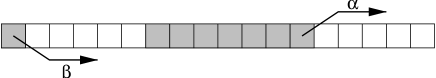
Figure 2: Schematic representation of a single jam. Cars are represented by grey cells and empty cells are white. $\alpha$ is the outflow of the jam. The inflow $\beta$ is generated by the outflow of a megajam at the left end.

In the next section we will introduce a stochastic theory of jamming based on random walk like arguments. Our approach gives the exact solution in the special case $p=0$ where the fluctuations of free flowing vehicles are completely suppressed. For the general case $0<p\ll p_{0}$ the results are in good agreement with simulations.

4 Random walk theory of jamming

The main object of our investigation is a sequence of $n$ cars at rest forming a compact jam (see Fig. 2). In every timestep the first car can leave the megajam with probability $\alpha=p_{0}$ according to the acceleration and randomization steps in the update algorithm (see Sec. 2). Additionally a new car is able to enter the jam at its end with probability $\beta$ which is determined by the vehicle distribution behind the jam. In general $\beta$ will be generated by the outflow of a megajam (see below).

The outflow $\alpha$ realized through $p_{0}$ is an independent identically distributed (i.i.d.) random variable. For simplicity we start with the case that $\beta$ is also an i.i.d. random variable. This condition is fulfilled if fluctuations of free flowing vehicles are completely suppressed, i.e., for $p=0$, and when the vehicle distribution behind the considered jam is generated by the outflow of a megajam. In this case we will consider open boundary conditions with an (infinite) megajam at the left end and an empty system at the right end (Fig. 2). The density in the free flow regime is then determined by the waiting time of the first car in the megajam. In this special case the gaps between the vehicles are always a multiple of their maximum velocity $v_{{\rm max}}$ since the waiting times are discrete and no interactions between cars occur in the outflow region for $p=0$. For example a waiting time of $t_{w}$ timesteps leads to a gap of $t_{w}\cdot v_{{\rm max}}$ cells. Then a car with this gap will reach the end of the jam exactly $t_{w}$ timesteps after its predecessor. It is obvious that the waiting times of the first car in the megajam determine directly the inflow $\beta$ into the analyzed jam which therefore can be treated as an i.i.d. variable. Note that the randomization parameter $\tilde{p}_{0}$ of cars standing in the megajam can be considered as a control parameter for the vehicle distribution in the free flow regime, i.e., the inflow $\beta=\beta(\tilde{p}_{0})$. Therefore it is in general different from the $p_{0}$ of the cars that have already left the megajam, i.e., the $p_{0}$ governing the resolution of the jam under consideration. In this way we can realize $\alpha\neq\beta$ for the open system. The case of periodic boundary conditions can be treated as a special case of the problem where in the jammed state the inflow into the jam is determined by the outflow out of the jam and hence $\alpha=\beta$. A detailed description of the initial and boundary conditions considered here as well as a discussion of the influence of deviating gap distributions in the inflow region (e.g. if $\beta$ is no longer an i.i.d. variable) will be given below.

In the following we will map the jam dynamics onto a random walk problem. The number of standing cars $n$ in the jam determines the position $n$ of a random walker. The walker moves on a discrete lattice in discrete time. A car leaving (entering) the jam then corresponds to one step to the left (right). In the following we determine the probability $\pi_{t,n}$ that a jam of width $n$ resolves after $t$ timesteps. Here a jam is considered to have resolved when the last remaining car accelerates.

In random walk terminology this problem is equivalent to the calculation of the first passage time of a walker starting at position $n_{0}=n(t=0)$. $\pi_{t,n}$ is the probability that walker at position $n$ reaches the origin $n=0$ of the system in $t$ timesteps. Taking into account that $\alpha$ and $\beta$ are i.i.d. random variables one gets the following master equation for the duration of the process until the random walker reaches the origin:

$$\pi_{t+1,n>1} = \alpha(1-\beta)\pi_{t,n-1}+\beta(1-\alpha)\pi_{t,n+1}+\left[(1-\alpha)(1-\beta)+\alpha\beta\right]\pi_{t,n},$$

$$\pi_{t+1,1} = \alpha\pi_{t,0}+\beta(1-\alpha)\pi_{t,2}+(1-\alpha)(1-\beta)\pi_{t,1}.$$ (2)

It is obvious that $\pi_{0,n_{0}>0}=0$ and that by definition $\pi_{1,1}=\alpha$ since a jam of length $n=1$ resolves with probability $\alpha$ in one timestep independent of the inflow. Furthermore we assume an absorbing barrier at the origin $\pi_{0,0}=1$, i.e. the process stops when the random walker reaches the origin (the jam is dissolved). Note, that the variable $n$ covers the whole spektrum of possible positions of a random walker during his movement, while $n_{0}$ denotes the starting position. For a discussion of the mathematical aspects of first passage time problems we refer to [25, 26].

As an example for the derivation of these equations consider a walker starting at position $n_{0}>1$. If the first trial results in a movement to the left the process continues as if the initial position had been $n_{0}-1$. A movement to the left means that a jam of width $n_{0}$ evolves into a jam of width $n_{0}-1$. This event occurs if the first car leaves the jam and no additional car enters it. The probability for this is $\alpha(1-\beta)$. Similarly, if the first trial results in a movement to the right the process continues as if the initial position had been $n_{0}+1$. The probability for a movement to the right is given by $\beta(1-\alpha)$, i.e., the first car remains in the jam and an additional car enters it. Furthermore the position of the walker, and thus the jam length, are unchanged if either one car leaves and one car enters the jam (probability $\alpha\beta$) or no car leaves and enters the jam (probability $(1-\alpha)(1-\beta)$). From the first equation of (2) we see that the random walk is symmetric (for $n>1$) if $\alpha(1-\beta)=(1-\alpha)\beta$. For $\alpha(1-\beta)>(1-\alpha)\beta$ the walker is biased to the left and the jam will dissolve quickly. For $\alpha(1-\beta)<(1-\alpha)\beta$ the bias is to the right and the jam will grow on average. But even in this case a complete resolution is possible through fluctuations.

In order to determine the probabilities we introduce the following generating functions:

$$\Pi_{n_{0}}(z)=\sum_{t=0}^{\infty}\pi_{t,n_{0}}z^{t}.$$ (3)

At this point it has to be taken into account that the case $n=1$ must be viewed separately. For a jam consisting of only one standing car the probability for resolving is equal to $\alpha$ (the standing car accelerates) even if a new car enters the minijam at its end. Therefore we will first look at the special case of a random walker starting at position $n_{0}=1$. A typical process in which the jam resolves after $t>1$ timesteps may be described as follows.
(I) The walker does not move for $\mu$ timesteps.
(II) Then the random walker moves one unit to the right.
(III) After the step to the right the walker first has to return to $n=1$ before the jam resolves, i.e. before the walker reaches $n=0$. The return to the initial position $n=1$ will take $\nu-1$ further timesteps ($\nu=2,3,\ldots$).
(IV) Now there are $t-\nu-\mu$ further timesteps left for the walker to reach the origin at last.
These three events are mutually independent and so the probability of the simultaneous realization of the three events is given by the product of the single probabilities.

We first look at the case $\mu=0$. The cases $\mu>0$ will later be taken into account iteratively. We start with the solution of event (III). Since in this case the position of the walker is always larger than one only the first equation of the system (2) has to be considered. In contrast to the general solution for event (III) the hopping probabilities do not depend on the position anymore. A random walker has to return to the origin (in this case $n=1$) starting from a position shifted one step to the right (here $n=2$). The solution of this homogeneous first passage time problem is described in [25, 26]. Assuming an absorbing barrier and introducing a separate generating function for event (III),

$$\tilde{\Pi}(z)=\sum_{t=0}^{\infty}\tilde{\pi}_{t,1}z^{t},$$ (4)

where $\tilde{\pi}_{t,1}$ is the probability that a walker starting at $n=2$ reaches $n=1$ for the first time after $t$ timesteps, the following solution for part (III) of the problem can be obtained:

$$\tilde{\Pi}(z) = \frac{1-\left[\alpha\beta+(1-\alpha)(1-\beta)\right]z}{2\beta(1-\alpha)z}$$ (5)

$$-\sqrt{\left[\frac{1-\left[\alpha\beta+(1-\alpha)(1-\beta)\right]z}{2\beta(1-\alpha)z}\right]^{2}-\frac{\alpha(1-\beta)}{\beta(1-\alpha)}}.$$

The return probability, i.e. the probability that the walker reaches $n=1$ at an arbitrary time, is then given by

$$\tilde{\Pi}(1)=\begin{cases}\frac{\alpha(1-\beta)}{\beta(1-\alpha)}&{\rm if\ }\alpha(1-\beta)\leq\beta(1-\alpha)\\ 1&{\rm if\ }\alpha(1-\beta)\geq\beta(1-\alpha).\end{cases}$$ (6)

As already discussed above, for $\alpha(1-\beta)>\beta(1-\alpha)$ the walker is biased to the left and will always reach $n=1$. For $\alpha(1-\beta)<\beta(1-\alpha)$, on the other hand, the walker is biased to the right and will only return with probability $\frac{\alpha(1-\beta)}{\beta(1-\alpha)}<1$.

Now the complete event (I)–(IV) occurs for some $\nu<t$. Summing over all possible $\nu$ one gets:

$$\pi_{t,1} = \beta(1-\alpha)\left[\tilde{\pi}_{1,1}\pi_{t-2,1}+\tilde{\pi}_{2,1}\pi_{t-3,1}+.....+\tilde{\pi}_{t-2,1}\pi_{1,1}\right]$$ (7)

$$+(1-\alpha)(1-\beta)\pi_{t-1,1}.$$

The last term takes into account event (I) for $\mu\neq 0$ since $(1-\alpha)(1-\beta)$ is the probability that a walker at site $n$ will not move. In the first term, $\beta(1-\alpha)$ is the probability of event (II). The quantity within the brackets is the probability of events (III) and (IV) for the allowed values of $\nu$. Note that it is the $(t-1)$-st term of the convolution $\{\pi_{t,1}\}\ast\{\tilde{\pi}_{t,1}\}$ (see [26]). After multiplying (7) with $z^{t}$ and summing over all times one finds an expression for the generating function (3) for $n_{0}=1$:

$$\Pi_{1}(z)=\frac{\alpha z}{1-(1-\alpha)(1-\beta)z-\beta(1-\alpha)\tilde{\Pi}(z)z}.$$ (8)

The probability for the complete return is given by $\Pi_{1}(1)$. Using equation (6) it is easy to obtain this quantity explicitly. The solution for the nontrivial case $\alpha(1-\beta)<\beta(1-\alpha)$ is given by

$$\Pi_{1}(1)=\frac{\alpha}{\beta}.$$ (9)

We now turn to the general case where one has to deal with starting positions greater than one, i.e. initial conditions consisting of more than only one standing car, $n_{0}>1$. Similarly to the foregoing approach the process of reaching the origin can be seen as the realization of mutually independent events. For instance, the probability that a random walker starting at position $n_{0}=2$ reaches the origin is given by the event that the walker reaches first position $n=1$ and thereafter reaches position $n=0$.

The general resolving process of a jam with an initial width $n_{0}$ standing cars can be described as a chain of processes leading finally to the case $n=1$. Thus using the generating functions (3) and (4) this convolution of events can be expressed through

$$\Pi_{n_{0}}(z)=\tilde{\Pi}(z)^{n_{0}-1}\Pi_{1}(z).$$ (10)

With equation (6) and (9) the following relation for the resolving probability of a jam of width $n$ can be obtained:

$$\Pi_{n_{0}}(1)=\frac{\alpha}{\beta}\left[\frac{\alpha(1-\beta)}{\beta(1-\alpha)}\right]^{n_{0}-1}.$$ (11)

Besides the resolving probability there is also another interesting quantity that is directly accessible through the generating function (10), namely the average lifetime $T_{n_{0}}$ of a jam of initial length $n_{0}$:

$$T_{n_{0}}=\sum_{t=0}^{\infty}t\pi_{t,n_{0}}=\Pi_{n_{0}}^{\prime}(1).$$ (12)

Using (10) one can obtain an explicit result for $T_{n_{0}}$. Figure 3 shows results for the resolving probability (11) and for the lifetime (12) of a jam for various initial widths $n_{0}$. The outflow parameter (fluctuation parameter of standing cars) is chosen such that $\alpha=0.5$ in both diagrams. In the left figure a strong dependence on the starting position of the walker (initial width of the jam) can be seen. Furthermore one can observe directly an outstanding difference between the case $n_{0}=1$ and $n_{0}>1$. While for $n_{0}>1$ the resolving probability fastly converges to zero for increasing $\beta$, this value is shifted to $\alpha$ for $n_{0}=1$. This shift can be explained through the update procedure of the model discussed above. A jam consisting of only one standing car resolves with probability $\alpha$ even if a new car enters the minijam at its end. The right part of Fig. 3 shows the mean disolving time for different $n_{0}$. It is obvious, that this quantity grows with increasing $n_{0}$ due to the fact, that the resolving process of a jam with $n_{0}$ standing can be described as a chain of resolving processes of smaller jams. Additionally it should be noted that a higher inflow $\beta$ leads to lower dissolving times, but it must be taken into account that the dissolution of a jam under a high inflow $\beta$ is a rather rare event.

Figure 3: Left: The dissolving probability of a jam (see Eqn. (11)) is illustrated for different $n_{0}$. It can clearly be seen that the dissolving probability strongly depends on the initial width $n_{0}$ of the jam, and that for the special case $n_{0}=1$ this quantity will never fall below $\alpha$. Right: The conditional mean dissolving time $T_{n_{0}}/\Pi_{n_{0}}(1)$ is shown for the set of $n_{0}$ used in the left part of the diagram. Note that the higher the inflow $\beta$ the lower the mean dissolving time, but the probability for dissolution on short times will shrink drastically. The outflow rate in both diagrams is set to $\alpha=0.5$.

5 Numerical results

In the previous section we have derived an analytical expression for the dissolution probability $\Pi_{n_{0}}(1)$ of a jam with an initial width of $n_{0}$ standing cars. To compare the analytical predictions with simulation results we use a damage scenario by initializing a finite jam into an undisturbed system. The reaction of the system to such disturbances is characterized by the sensitivity $S=1-\Pi_{n_{0}}(1)$. The sensitivity is simply the probability that a cluster of $n_{0}$ standing cars causes a wide jam (for open boundary conditions) or leads to the jammed state of the system (for periodic boundary conditions). The following initial conditions are considered to produce an area of free flowing vehicles in the density regime $\rho_{1}<\rho<\rho_{2}$. Remember that the mean inflow into the induced minijam will always be greater than the mean outflow in this area.

(A) Here we set the randomization parameter $p$ of moving cars to zero, i.e. fluctuations in free flow are suppressed. We choose an open system with a sufficiently large megajam at the left boundary in this scenario. The gap distribution is than realized through the outflow of this megajam and fluctuations of free flowing vehicles are completely suppressed. The randomization parameter $\tilde{p}_{0}$ of standing cars in the megajam is used as control parameter for $\beta$. After a car has left the megajam it is therefore reset to $p_{0}$. Thus the distance between two consecutive cars is always a multiple of $v_{{\rm max}}$ whereby the inflow into the damage is an i.i.d. random variable in that case in correspondence to the theory.
(B) Also in the second case the free-flow car distribution is generated through a megajam, but fluctuations are permitted, i.e., $p>0$. Hence the gap distribution contains values deviating from $n\cdot v_{{\rm max}}$ due to velocity fluctuations or braking events.
(C) Finally, a homogeneous initialization of cars in a periodic system is considered. Simulations for this situation are performed until the system has relaxed into its free-flow steady state. As a result of the dynamics this steady state shows large deviations in the gap distribution in comparison to the megajam initializations.
Note that the inflow into the induced minijam is controlled in the cases (A)+(B) through the randomization parameter of standing cars at the left boundary (megajam) while in case (C) the inflow is controlled indirectly through the density of the homogeneous initialization. The inflow $\beta$ can be obtained easily in the simulations.

After the free-flowing vehicles are initialized according to the scenarios described above we induce a damage in the system by setting the velocity of a randomly chosen vehicle to zero. The acceleration of this stopped car is suppressed in the following update steps until the damage grows to $n_{0}$ cars. Now, the system is updated according to the update rules without any further outer influences. The damage considered can either grow to a large jam or dissolve.

In Fig. 4 we show the simulated sensitivity $S=1-\Pi_{n_{0}}(1)$ and the mean resolving time for the different initial conditions and compare these results to the analytical predictions of Sec. 4. It is clear that for scenario (A) the analytical results are exact. Even scenario (B) shows an excellent agreement with the analytical curve, but small deviations occur due to the fact that the inflow is no i.i.d. random variable anymore although the mean inflow is still identical to that of scenario (A). Furthermore it should be noted that for the considered dissolution of a small damage the time scale is small, so that local deviations in the gap distribution can play an important role. In the case of the homogeneous initialization (C) we found larger deviations from the analytical curve. The origin of this discrepancy is also the gap distribution which in contrast to the megajam initializations is not generated through a stochastic outflow parameter. Instead it is determined by vehicle interactions due to the model dynamics (simulation runs until relaxation). Hereby repulsive forces between the cars lower the probability of finding large gaps. Therefore the theory overestimates the dissolving probability in the case of a periodic system with homogeneous starting conditions (C). Note, that for large $p$ spontaneous jams can appear in the free flow region before a car is able to enter the induced minijam (starting condition (B)) or in the case of homogeneous initialization (C) jams can appear in the system before the steady state is reached. Therefore we do not consider initializations with higher $p$ in this work. Our aim was to analyze the dynamics of a single jam. Thus we chose the VDR model which exhibits phase separation but only for $p_{0}\gg p$. Nonetheless we want to point out that the random walk approach for the dynamics of a single jam seems to be generic for various stochastic CA models for traffic flow.

Figure 4: The outflow rate in both diagrams is set to $\alpha=0.5$ and a width of $n_{0}=4$ is chosen for the induced minijam. We performed $10^{5}$ simulation runs (induced minijams) for every data point. Left: The probability that the initial minijam grows to a wide jam is illustrated for different starting conditions. The analytical curve is given by $S=1-\Pi_{n_{0}(1)}$ (see Eqn. (11)). Right: The mean dissolution time of the initial minijam is shown in the left part of the diagram.

6 Summary

We have analyzed the VDR model which exhibits phase separation and metastable states in order to obtain a deeper insight into the jamming behavior in cellular automata models for traffic flow. An analytical approach in terms of random walk theory has been suggested to determine characteristic quantities of wide jams, especially resolving probabilities and lifetimes. The analytical results reveal interesting peculiarities of the model. One finds, e.g., a shift in the convergence of the dissolving probability going from $n_{0}=1$ to greater values of $n_{0}$. The analytical predictions are compared to simulation results. For this purpose a damage scenario is considered by initializing a finite single jam into an undisturbed system. Different boundary conditions are assumed in our investigations. In one case we choose open boundary conditions whereby the free-flow car distribution is generated through the outflow of a sufficiently large megajam at the left boundary. Additionally, a periodic system with homogeneous initialization is considered. In this case the gap distribution is generated through the dynamics of the model (simulation are performed until the system has relaxed). For the megajam initialization we found a very good or even exact agreement between simulation and theory. The homogeneous initialization with periodic boundary condition shows larger deviations from the predicted curve but the overall agreement also rather good. We stress that the random walk approach renders the jamming dynamics of the model. Nagel and Paczuski [16] also analysed the lifetime of jams in another stochastic CA model for traffic flow, the cruise control limit of the NaSch model, and found good agreement with random walk theory. Therefore we assume that the jamming behavior is generic for a lot of the stochastic CA models for traffic flow.

Furthermore, the fact that one can interpret the emergence of wide jams in terms of probability theory points out a main difference between stochastic CA models for traffic flow and hydrodynamical approaches. To explain the major differences we want to focus on the hydrodynamical model introduced by Kerner and Konhäuser [12]. Although the VDR model invokes most of the characteristic properties (i.e., linear growth of emerging jams, moving transition layer, …) of jams in fluid-dynamical models the formation of large jams due to local perturbations is completely different. In the hydrodynamical model a wide jam is formed from an initially homogeneous state through an external damage which exceeds a critical size. This critical size strongly depends on the density whereby damages below this size dissolve and damages above the critical size lead to wide jams. In contrast, in the VDR model an induced damage leads to a wide jam only with a certain probability. There is no quantity like a critical value for the formation of jams but the probability that a damage causes a jam of course depends on the size of the damage and the density of the initial homogeneous state. Additionally one finds spontaneous jam formation without external influences due to velocity fluctuations in the metastable branch of the model.

To conclude, the results presented here are of practical relevance for various applications of traffic flow using stochastic CA models. Due to its simplicity this class of models has become popular for large scale computer simulation (city or highway networks). Complex networks usually contain many bottlenecks such as crossings, lane reductions, traffic lights or traffic signs. Therefore induced jams often play an important role in realistic traffic scenarios and a proper understanding of the jamming process and dynamics is benefitable.

References

- [1] C.F. Daganzo, M.J. Cassidy, and R.L. Bertini, Transp. Res. A 33, 365 (1999)
- [2] D. Helbing, Verkehrsdynamik: Neue Physikalische Modellierungskonzepte, (in German) (Springer, 1997)
- [3] J. Treiterer, Ohio State Technical Report No. PB 246094, (1975)
- [4] B.S. Kerner and H. Rehborn, Phys. Rev. E53, (1996)
- [5] B.S. Kerner and H. Rehborn, Phys. Rev. Lett. 79, 4030 (1997)
- [6] B.S. Kerner, Phys. Rev. Lett. 81, 3797 (1998)
- [7] L. Neubert, L. Santen, A. Schadschneider, and M. Schreckenberg, Phys. Rev. E60, 6480 (1999)
- [8] D.E. Wolf, M. Schreckenberg, and A. Bachem (eds.), Traffic and Granular Flow (World Scientific, 1996)
- [9] M. Schreckenberg and D.E. Wolf (eds.), Traffic and Granular Flow ‘97 (Springer, 1998)
- [10] D. Helbing, H.J. Herrmann, M. Schreckenberg and D.E. Wolf (eds.), Traffic and Granular Flow ‘99 (Springer, 2000)
- [11] D. Chowdhury, L. Santen, and A. Schadschneider, Phys. Rep. 329, 199 (2000) and Curr. Sci. 77, 411 (1999)
- [12] B.S. Kerner, S.L. Klenov, and P. Konhäuser, Phys. Rev. E 56, 4200 (1997)
- [13] K. Nagel and M. Schreckenberg, J. Physique I 2, 2221 (1992)
- [14] R. Barlovic, L. Santen, A. Schadschneider, and M. Schreckenberg, Eur. Phys. J. B5, 793 (1998)
- [15] W. Knospe, L. Santen, A. Schadschneider, and M. Schreckenberg, J. Phys. A (in press)
- [16] K. Nagel and M. Paczuski, Phys. Rev. E51, 2909 (1995)
- [17] A. Schadschneider, Eur. Phys. J. B10, 573 (1999)
- [18] R. Barlovic, Diploma Thesis, Universität Duisburg (1998)
- [19] L. Santen, Ph.D. Thesis, Universität zu Köln (1999)
- [20] A. Pottmeier, Diploma Thesis, Universität Duisburg (2000)
- [21] A. Pottmeier, R. Barlovic, W. Knospe, A. Schadschneider, and M. Schreckenberg, in preparation
- [22] G. Diedrich, Diploma Thesis, Universität zu Köln (1999)
- [23] G. Diedrich, L. Santen, A. Schadschneider, and J. Zittartz, to be published
- [24] L. Neubert, H.Y. Lee, and M. Schreckenberg, J. Phys. A32, 6517 (1999)
- [25] N.G. van Kampen, Stochastic Processes in Physics and Chemistry (North-Holland, 1992)
- [26] W. Feller, An Introduction to Probability Theory and Its Applications, Volume I, (Wiley Series, 1968)