Spin polarization and magneto-luminescence of confined electron-hole systems

Abstract

A BCS-like variational wave-function, which is exact in the infinite field limit, is used to study the interplay among Zeeman energies, lateral confinement and particle correlations induced by the Coulomb interactions in strongly pumped neutral quantum dots. Band mixing effects are partially incorporated by means of field-dependent masses and g factors. The spin polarization and the magneto-luminescence are computed as functions of the number of electron-hole pairs present in the dot and the applied magnetic field.

I Introduction

In the present paper, we study the spin polarization and the magneto-luminescence of a neutral, medium-size quantum dot (qdot) subjected to a strong (pulsed) laser pumping and a strong magnetic field. There are many good reasons to study the properties of this system.

On one hand, recent magneto-tunneling experiments oosterkamp ; haw have stated very clearly the role of Zeeman energies, lateral confinement and Coulomb repulsion in the spin polarization of a qdot filled with $N$ electrons. At “filling factors” $2>\nu\gtrsim 1$, ground-state rearrangements lead to significant oscillations of the conductance peak positions as a function of the magnetic field. The situation could be even more interesting for electron-hole (e-h) clusters, where additional e-h correlations come into play. Traces of spin rearrangements shall be seen in the luminescence and other optical properties.

On the other hand, extensive measurements of quantum well (qwell) luminescence exist for different e-h densities (laser excitation power) and polarizations lumin . A BCS-based theory has been proposed tejedor . Very high magnetic fields, up to 60 T, have been applied mainly to low-density systems, and the results have been interpreted in terms of isolated neutral and negatively charged excitons kim1 . Analogous experiments in qdots are lacking, but the available experimental resources are enough to create a high population of excitons in a medium-size qdot in a strong magnetic field. 6-exciton luminescence has been undoubtedly observed in single small InAs quantum dots at $B=0$ gershoni . In qwells, very high e-h densities ($10^{13}$ pairs/cm²) have been achieved with pulsed pumping kim2 .

Our model quantum dot is made up from a symmetrical GaAs-AlGaAs quantum well, 8.5 nm wide in the growth direction. Stress is supposed to induce a lateral confinement, which is described by a parabolic potential with $\hbar\Omega\approx 1.2$ meV. An electron-hole system is created in the dot by a strong 5 ps pulsed laser, as it is experimentally done for example in Ref.kim2, . The mean lifetime of this system is around hundred of ps or even longer, i. e. a time scale much greater than the characteristic times ($\approx$ 1 ps) to reach equilibrium time . Thus, at very low temperatures we end up with an “stable” $N$-pair e-h cluster in its ground state.

Results for spin-up and -down densities, hole and electron spin polarizations and for the position and magnitude of the coherent luminescence peak as functions of the magnetic field and of the mean number of excitons are presented below. The theoretical framework used is a BCS-like wave function, corrected against particle number non-conservation by means of a Lipkin-Nogami procedure LN ; yo . This wave function is able to reproduce the expected “Bose condensed” state in the $B\to\infty$ limit lerner ; dzyubenko ; paquet . A big basis of one-particle states is used, which includes up to 3 Landau levels and 202 states per Landau level. We consider systems with up to 40 e-h pairs.

The plan of the paper is as follows. In Section II, the model to be employed is described in details. The basics of our theoretical scheme are summarized in Section III. In Section IV, the main results are presented and discussed. Concluding remarks are given in the last section.

II The Model

We consider a system of $N$ electrons and $N$ holes confined in a quasi two-dimensional quantum dot, and in the presence of a perpendicular magnetic field. As mentioned above, the qdot is made up from a 85 Å-wide symmetric qwell. A parabolic potential confines the motion of the particles in the plane perpendicular to the grow direction. The first qwell sub-band approximation is used, i. e. the confining energies along the $z$ direction are written as $E_{e(h)}^{z}=\frac{\hbar^{2}\pi^{2}}{2m_{e(h)}L_{z}^{2}}k_{e(h)}^{2}$, with $k_{e(h)}=1$. Notice that for the $85$ Å-width GaAs well, the gap to the second qwell state is $\Delta E_{e}^{z}\approx 210$ meV, and $\Delta E_{h}^{z}\approx 39$ meV for electrons and holes respectively, whereas the typical Coulomb energy is $E_{Coulomb}\approx 3.18\sqrt{B[T]}$ meV. This model is a common theoretical framework in the study of strained or self-assembled quantum dots qdot . By using the symmetric gauge, $\vec{A}(\vec{r})=\frac{\vec{B}\times\vec{r}}{2}$, dimensionless coordinates, $\vec{r}\rightarrow l_{B}\vec{r}$, with $l_{B}=\sqrt{2\hbar c/eB}$, and using Landau level (LL) states $\left\{|i\rangle=|n_{i},m_{i},s_{i}\rangle\right\}$ ($n_{i}=0,1,\cdots;\;\;m_{i}=-\infty,\cdots,-1,0,1,\cdots,\infty;$ and $s_{i}=\pm 1/2$ are the radial, angular momentum and spin quantum numbers, respectively) as set of one-particle states, we can write the Hamiltonian in second quantization as:

$$H = \sum_{i}\left\{\frac{\hbar\omega_{c}^{e}}{2}\varepsilon_{i}^{e}+E_{e_{i}}^{Zeeman}\right\}e_{i}^{{\dagger}}e_{i}$$ (1)

$$+ \sum_{i}\left\{\frac{\hbar\omega_{c}^{h}}{2}\varepsilon_{i}^{h}+E_{h_{i}}^{Zeeman}\right\}h_{i}^{{\dagger}}h_{i}$$

$$+ \sum_{ij}\hbar\langle i|\vec{r}^{2}|j\rangle\left\{\frac{\Omega^{2}}{\omega_{c}^{e}}e_{i}^{{\dagger}}e_{j}+\frac{\Omega^{2}}{\omega_{c}^{h}}h_{i}^{{\dagger}}h_{j}\right\}$$

$$+ N\left\{E_{gap}+E_{e}^{z}(k_{e}=1)+E_{h}^{z}(k_{h}=1)\right\}$$

$$+ \frac{e^{2}}{\epsilon l_{B}}\left\{\frac{1}{2}\sum_{ijkl}\langle ij|\frac{1}{\left|\vec{r}\right|}|kl\rangle e_{i}^{{\dagger}}e_{j}^{{\dagger}}e_{l}e_{k}\right.$$

$$+ \frac{1}{2}\sum_{ijkl}\langle ij|\frac{1}{\left|\vec{r}\right|}|kl\rangle h_{i}^{{\dagger}}h_{j}^{{\dagger}}h_{l}h_{k}$$

$$- \left.\sum_{ijkl}\langle ij|\frac{1}{\left|\vec{r}\right|}|kl\rangle e_{i}^{{\dagger}}h_{j}^{{\dagger}}h_{l}e_{k}\right\},$$

where $m_{e}(m_{h})$ are the electron and hole effective masses, $\Omega$ is the dot confining frequency, and $\epsilon$ is the dielectric constant. $E_{gap}$ is the gap separation between the conduction and valence bands, $E^{Zeeman}_{e_{i}(h_{i})}=\pm g_{e(h)}\mu Bs_{i}^{e(h)}$, with $g_{e(h)}$ the effective g-factors, $\mu$ is the Bohr magneton, $s_{i}^{e(h)}$ are the $z$-components of the ith particle spin, $\varepsilon_{i}^{e(h)}=2n_{i}+|m_{i}|\pm m_{i}+1$ are the LL energies for electrons (holes), $\omega_{c}^{e(h)}=eB/m_{e(h)}c$ is the electron (hole) cyclotron frequency, and $e_{i}(h_{i}),\;e_{i}^{{\dagger}}(h_{i}^{{\dagger}})$ are the electron (hole) destruction and creation operators. Conventionally, we write $s_{h}=\pm 1/2$ for the two branches of the heavy hole sub-band. To the electronic $j_{z}=-3/2$, for example, we ascribe $s_{h}=1/2$.

The effective parameters entering the Hamiltonian (masses and g factors) are magnetic field- and width-dependent magnitudes to approximately account for band mixing. For the $85$ Å well, we fitted the experimental in-plane heavy hole mass mh , thus obtaining:

$$m_{h}^{85\mbox{\AA}}(B)=\left\{\begin{array}[]{ll}0.17,&\mbox{for $B<10$ T}\\ \frac{0.17+0.0168B}{1+0.023B},&\mbox{for $B>10$ T}.\end{array}\right.$$ (2)

Experimentally, the dependence of the electron g-factor on well width and magnetic field is well determined ge5 ; ge1 ; ge2 ; ge3 ; ge4 , and in our case we have:

$$g_{e}^{85\mbox{\AA}}(B)=-0.1667+0.0052\;B[\rm{T}].$$ (3)

The dependence of the hole g-factor on the magnetic field for high $B$ values, however, is not properly determined ge2 ; ge3 . Here we assume a linear behavior with the field, as in the electron case, and fitted it to                                     kim1 . The result is

$$g_{h}^{85\mbox{\AA}}(B)=-0.05\;B[\rm{T}].$$ (4)

Notice that in the $B\to 0$ limit, $g_{h}$ vanish because the exciton (X) g-factor, defined as $g_{X}=g_{e}+g_{h}$, and the electron g-factor are equal in the $85$ Å width wellge2 .

With this parameterization, $g_{e}$ changes sign at $B_{c}\approx 32$ T. Consequences of this facts are discussed below.

III The BCS scheme

The BCS approach has been successfully applied by Paquet et. al. in the study of the two-dimensional (2D) e-h system paquet , and by Fernández-Rossier and Tejedor to the exciton gas in a qwelltejedor . We used it previously in the study of finite e-h systems at zero magnetic field yo . We employ the Lipkin-Nogami (LN) scheme to avoid particle number non-conservation in a finite system. The BCS wave function is given by

$$|BCS\rangle_{N}=\prod_{i}\left(u_{i}+v_{i}e_{i}^{{\dagger}}h_{\bar{\imath}}^{{\dagger}}\right)|0\rangle_{h}|0\rangle_{e}~{}~{},$$ (5)

where $|0\rangle_{h}(|0\rangle_{e})$ are the respective electron (hole) vacuum. The subscript “$N$” in the BCS function means that the average number of pairs is just $N$, i.e. $\langle\hat{N}\rangle=\langle BCS|\hat{N}|BCS\rangle_{N}=N$. $u_{i}$ and $v_{i}$ are the variational parameters. They fulfill the normalization conditions $u_{i}^{2}+v_{i}^{2}=1,\;\forall i$. The hole state $|\bar{\imath}\rangle$ which is paired with the electron state $|i\rangle=|n_{i},m_{i},s_{i}\rangle$ is different for the two magnetic field regimes, reflecting the ground state spin structure, as it is show in Fig. 1. For $B<32$ T, electrons and holes with opposite spins are paired, then $|\bar{\imath}\rangle=|n_{i},-m_{i},-s_{i}\rangle$. Whereas for $B>32$ T, the energy is minimized when the $|i\rangle$ electronic state is paired with $|\bar{\imath}\rangle=|n_{i},-m_{i},s_{i}\rangle$.

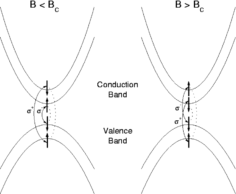
Figure 1: Schematics of the spin sub-band structure for the two field regimes. The dotted lines show the paired electron and hole states in the BCS wave function. The interband optical transitions for the two circular polarizations of light $\sigma^{\pm}$ are indicated.

The total angular momentum (projection onto the z axis), corresponding to $|BCS\rangle_{N}$ is zero because the angular momentum of each pair is zero. The total electron or hole spin, however, depend on the populations of spin-up and down components.

The detailed description of the LN method can be found in Refs. LN ; yo . For completeness, we sketch the main results. The LN estimate for the ground state energy is given by:

$$E_{LN}=E_{BCS}-2\lambda_{1}(\langle\hat{N}\rangle-N)-\lambda_{2}(\langle\hat{N}^{2}\rangle-N^{2}),$$ (6)

where $E_{BCS}$ is the expectation value of the effective Hamiltonian $\hat{H}=H-N\left\{E_{gap}-E_{e}^{z}(k_{e}=1)-E_{h}^{z}(k_{h}=1)\right\}$ in $|BCS\rangle_{N}$:

$$E_{BCS} = \mbox{}_{N}\langle BCS|\hat{H}|BCS\rangle_{N}$$ (7)

$$= \sum_{i}\left\{\frac{\hbar\omega_{c}^{e}}{2}\varepsilon_{i}^{e}+\frac{\hbar\Omega^{2}}{\omega_{c}^{e}}\varepsilon_{i}^{OA}+g_{e}\mu Bs_{i}^{e}\right\}v_{i}^{2}$$

$$+ \sum_{\bar{\imath}}\left\{\frac{\hbar\omega_{c}^{h}}{2}\varepsilon_{\bar{\imath}}^{h}+\frac{\hbar\Omega^{2}}{\omega_{c}^{h}}\varepsilon_{\bar{\imath}}^{OA}-g_{h}\mu Bs_{\bar{\imath}}^{h}\right\}v_{i}^{2}$$

$$- \frac{e^{2}}{\epsilon l_{B}}\left\{\sum_{i\neq j}\langle ij|\frac{1}{\left|\vec{r}\right|}|ji\rangle\left(v_{i}^{2}v_{j}^{2}+v_{i}u_{i}v_{j}u_{j}\right)\right.$$

$$- \left.\sum_{i}\langle ii|\frac{1}{\left|\vec{r}\right|}|ii\rangle v_{i}^{2}\right\}.$$

Notice that in the second term, the sum runs over hole states $|\bar{\imath}\rangle$. $\varepsilon_{i}^{e}=\varepsilon_{\bar{\imath}}^{h}=2n_{i}+|m_{i}|+m_{i}+1$ are the one-particle energies, and $\varepsilon_{i}^{OA}=\varepsilon_{\bar{\imath}}^{OA}=2n_{i}+|m_{i}|+1=\langle i|\vec{r}\,^{2}|i\rangle$ is the expectation value of the harmonic potential. The mean value of the number of pairs is

$$N = \langle\sum_{i}e_{i}^{{\dagger}}e_{i}\rangle_{BCS}=\langle\sum_{i}h_{i}^{{\dagger}}h_{i}\rangle_{BCS}$$ (8)

$$= \sum_{i}v_{i}^{2}.$$

The extrema conditions can be written in the standard form of gap equations

$$\Delta_{i}=\frac{e^{2}}{\epsilon l_{B}}\sum_{j(j\neq i)}\langle ij|\frac{1}{|\vec{r}|}|ji\rangle\frac{\Delta_{j}}{2\sqrt{\Delta_{j}^{2}-(\epsilon_{i}^{HF}-\mu)^{2}}},$$ (9)

where the Hartree-Fock energies are given by

$$\epsilon_{i}^{HF} = \frac{1}{4}(\hbar\omega_{c}^{e}+\omega_{c}^{h})(2n_{i}+|m_{i}|+m_{i}+1)$$ (10)

$$+ \frac{1}{2}\left(\frac{\hbar\Omega_{e}^{2}}{\omega_{c}^{e}}+\frac{\hbar\Omega_{h}^{2}}{\omega_{c}^{h}}\right)(2n_{i}+|m_{i}|+1)$$

$$+ \frac{\mu}{2}B(g_{e}s_{i}-g_{h}s_{\bar{\imath}})-\frac{e^{2}}{2\epsilon l_{B}}\langle ii|\frac{1}{\left|\vec{r}\right|}|ii\rangle$$

$$- \frac{e^{2}}{\epsilon l_{B}}\sum_{j(j\neq i)}\langle ij|\frac{1}{\left|\vec{r}\right|}|ji\rangle v_{j}^{2}-\lambda_{2}(N-v_{i}^{2}),$$

and we have used the usual BCS parameterization

$$v_{i}^{2}=\frac{1}{2}\left(1-\frac{\epsilon_{i}^{HF}-\mu}{\sqrt{\Delta_{i}^{2}-(\epsilon_{i}^{HF}-\mu)^{2}}}\right).$$ (11)

The chemical potential $\mu=\lambda_{1}+\lambda_{2}/2$ was introduced to fix the particle number, and $\lambda_{2}$ is determined in the LN scheme as:

$$\lambda_{2} = \left\{\langle\hat{H}\hat{N}^{2}\rangle\left(N^{2}-\langle\hat{N}^{2}\rangle\right)+\langle\hat{H}\hat{N}\rangle\left(\langle\hat{N}^{3}\rangle-\langle N\hat{N}^{2}\rangle\right)\right.$$ (12)

$$+ \left.\langle\hat{H}\rangle\left(\langle\hat{N}^{2}\rangle^{2}-\langle N\hat{N}^{3}\rangle\right)\right\}\left\{\langle\hat{N}^{2}\rangle^{3}+\langle\hat{N}^{3}\rangle^{2}\right.$$

$$+ \left.N^{2}\langle\hat{N}^{4}\rangle-\langle\hat{N}^{2}\rangle\left(2N\langle\hat{N}^{3}\rangle+\langle\hat{N}^{4}\rangle\right)\right\}^{-1},$$

where the expectation values $\langle\cdots\rangle$ are taken in the $|BCS\rangle_{N}$ state. The resulting equations are solved iteratively up to a precision of $10^{-12}$ in $\epsilon_{i}^{HF}$. Calculations were performed for $20\leq N\leq 40$ pairs and $606$ one-particle LL states.

Figure 2: Dependence of $E_{opt}-E_{dark}$ with the magnetic field. In figures 2 - 5, results for the $N=40$ exciton system are presented.

IV Polarization and magneto-luminescence

As shown below, the spin polarization of the electronic subsystem increases as the magnetic field is increased. At $B=32$ T, the electronic $g$-factor changes sign according to Eq. 3, leading to a rearrangement of electron-hole pairing in the absolute ground state. The kind of pairing minimizing the energy is represented in Fig. 1 by dashed lines. For $B>32$ T, the ground state is dark, and it is not even clear whether it can be reached by means of light excitation followed by spin relaxation processes. Thus, besides the ground state, for $B>32$ T, we compute also the lowest BCS state with $\sigma^{+}$ and $\sigma^{-}$ excitons. Below, we present results for the $N=40$ system, obtained with three LLs and 202 states per level, i. e. a total of 606 one-particle states.

As mentioned above, two BCS functions may be constructed. One in which optical excitons are formed, and a second one in which dark excitons are formed. The difference $E_{opt}-E_{dark}$ is drawn in Fig. 2 as a function of $B$, showing that the dark state becomes the ground state when the value $B\approx 32$ T is crossed and the electronic sub-bands are re-ordered. The absence of efficient spin relaxation mechanisms may, however, prevent the actual ground state to be occupied.

Figure 3: Spin-up and down densities. (a) Ground state at $B=20$ T, (b) Ground (dark) state at $B=40$ T, and (c) Excited (optically active) state at $B=40$ T.

It is interesting to note that the difference $E_{opt}-E_{dark}$, in the magnetic field interval shown in Fig. 2 is very close to the difference between the electronic Zeeman energies. A simple qualitative picture can be offered for the understanding of this and the next figures. The properties of the system are roughly determined by the holes because of the competition among the hole Zeeman energies and the total harmonic and Coulomb energies. The hole occupations are thus very similar for optical and dark states. The form of e-h pairing provides the “fine structure”. That is, the minimization of the energy leads to a definite pairing.

Scaled spin-up and -down densities, obtained from

$$\rho_{e}^{(\uparrow,\,\downarrow)}(\vec{r}) = \sum_{i=\{n_{i},m_{i},(\uparrow,\,\downarrow)\}\atop j=\{n_{j},m_{j},(\uparrow,\,\downarrow)\}}\phi_{i}^{e}(\vec{r})\phi_{j}^{e}(\vec{r})\>\mbox{}_{N}\langle BCS|e_{i}^{{\dagger}}e_{j}|BCS\rangle_{N}$$

$$= \frac{e^{-r^{2}}}{\pi}\sum_{i=\{n_{i},m_{i},(\uparrow,\downarrow)\}}\frac{n_{i}!\,r^{2|m_{i}|}\,v_{i}^{2}}{(n_{i}+|m_{i}|)!}\left[L_{n_{i}}^{|m_{i}|}(r^{2})\right]^{2},$$

are shown in Fig. 3. At $B=40$ T, we show the ground (dark) and optically-active excited-state densities, which are almost inverted in agreement with the argument given above. Notice that there are only four excess spin-up electrons at $B=20$ T. These small net polarizations for high magnetic fields are related to the attractive character of the e-h interaction. Unlike pure electron systems, small-radius orbits maximize e-h attraction, and the competition between Zeeman and Coulomb energies starts at higher fields.

The “hole dominance picture” leads to changes in the polarization, as $B$ is increased, through the reconstruction of the droplet edge, in a way very similar to electrons near filling factor one edge . This fact is illustrated in Fig. 4, where the difference between ground-state spin-up and -down densities for different values of $B$ are shown. It is evident that polarized densities differ mainly at the edge, and that changes in the polarization are more significant at the edge.

Figure 4: Difference between ground-state spin-up and -down densities for various magnetic field values.

The following two figures, Figs. 5 and 6, contain the main results of our paper. Electron and hole spin polarizations are drawn in Fig. 5a as a function of $B$. Solid lines refer to the ground state, while the dashed lines for $B>32$ T refer to the optically active state. Notice that even at a high field value like 45 T, the electronic polarization is only 70 %. Notice also the change in sign of the ground-state electronic spin at $B=B_{c}$. The inset shows the total ground-state spin squared, computed from

$$\langle\vec{S}_{e}^{2}\rangle_{BCS}=\frac{3}{4}N+\sum_{i,j}s_{i}s_{j}v_{i}^{2}v_{j}^{2}-\sum_{i}s_{i}v_{i}^{4}+\frac{1}{2}\sum_{\alpha}v_{\alpha\uparrow}^{2}v_{\alpha\downarrow}^{2}.$$ (14)

Figure 5: (a) Electron and hole spin polarizations. For $B>32$ T, both ground-state (solid line) and excited-state (dashed line) properties are drawn. The inset shows the total electron spin squared. (b) Luminescence intensities for both $\sigma^{-}$ and $\sigma^{+}$ polarizations.

The total (coherent) magnetoluminescence intensity for both $\sigma^{+}$ and $\sigma^{-}$ polarizations is presented in Fig. 5b. We compute it for $\sigma^{-}$ polarization, for example, from the expression

$$I_{total}^{\sigma^{-}} = \sum_{f}\Bigl{|}\,\mbox{}_{N-1}\langle f|P_{\sigma^{-}}|BCS\rangle_{N}\,\Bigr{|}^{2}$$ (17)

$$\propto \mbox{}_{N}\langle BCS|P_{\sigma^{-}}^{\dagger}\,P_{\sigma^{-}}|BCS\rangle_{N}$$

$$= \left\{\begin{array}[]{ll}\sum_{\alpha}v_{\alpha\uparrow}^{4}+\left(\sum_{\alpha}u_{\alpha\uparrow}v_{\alpha\uparrow}\right)^{2},&\mbox{bright state}\\ \sum_{\alpha}v_{\alpha\uparrow}^{2}v_{\alpha\downarrow}^{2},&\mbox{dark state},\end{array}\right.$$

where $|f\rangle$ is a basis of $N-1$ particle states , $\alpha=(n,\,m)$ is a composed index and, $P_{\sigma^{-}}=\sum_{\alpha}e_{\alpha\uparrow}h_{\bar{\alpha}\downarrow}$ is the interband dipole transition operator for the $\sigma^{-}$ circularly polarized light. Notice that $I_{total}$ is the integrated luminescence, corresponding to the transition from the given initial BCS state to any final state. The convention for solid and dashed lines is the same as in Fig. 5a. It shall be stressed that the degree of polarization, defined from

$$\frac{I_{total}^{\sigma^{-}}-I_{total}^{\sigma^{+}}}{I_{total}^{\sigma^{-}}+I_{total}^{\sigma^{+}}},$$ (18)

follows very well the behaviour of $\langle S_{z}\rangle$, i. e. the difference between the occupation of spin-up and -down sub-bands. This polarization is nearly 10 % at 20 T, and around 70 % at 45 T.

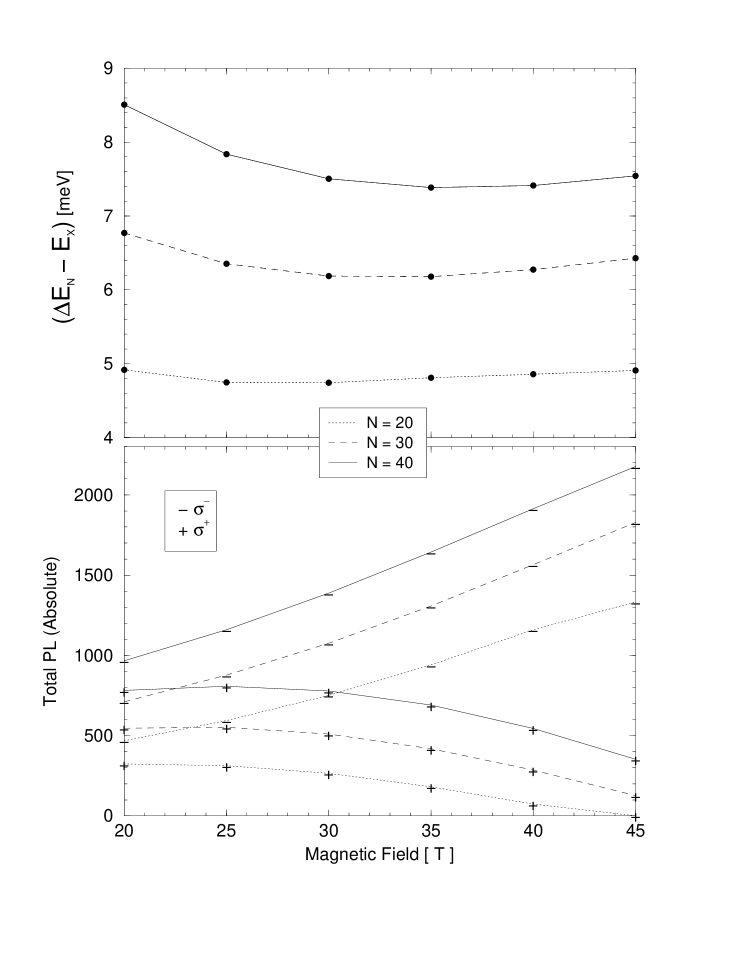
Figure 6: Dependence of the position of the luminescence line (see main text) and the intensities on the number of pairs in the dot. $E_{X}$ is the $\sigma^{-}$ exciton energy.

Finally, in Fig. 6 we show results for the position of the luminescence line and the intensities as functions of the numbers of pairs in the dot. In our computations, the energy is corrected against non-conservation of the total number of excitons, $N$. Conservation of the number of $\sigma^{+}$ and $\sigma^{-}$ excitons is not properly taken into account. Thus, we can not exactly compute the position of the $\sigma^{+}$ and $\sigma^{-}$ lines. In place of it, we show in Fig. 6a the difference $\Delta E_{N}=E_{LN}(N)-E_{LN}(N-1)$ relative to the exciton $\sigma^{-}$ line, $E_{X}$. The following interesting properties can be noticed in this figure: a) A blueshift as the number of excitons is raised kim2 . It is around 0.2 meV/exciton at $N=20$, and 0.15 meV/exciton at $N=30$, and b) An apparent minimum of each curve at $B$ around 30 T, i. e. at $B_{c}$. On the other hand, the intensity (Fig. 6b) shows an increase with $N$ for both polarizations, as one would expect from coherent emission.

V Concluding remarks

We have computed the spin polarization and the luminescence of a quantum dot in which a mean number of electron-hole pairs, $N$, have been created by a laser pulse. Band mixing effects were approximately taken into account by means of well width- and magnetic field-dependent masses and $g$-factors. For the model under study, the electron $g$-factor vanishes at $B_{c}\approx 32$ T. It means that, for magnetic field values around $B_{c}$, the electron polarization, and thus the ratio of intensities given by formula (18), is determined as a result of the interplay among Coulomb, confinement and hole Zeeman energies. The net polarization is only 70 % at $B=45$ T because of the attractive electron-hole interaction.

The general features found in our calculations, i. e. relatively small polarizations even at high magnetic field values, blueshift of the luminescence lines with an increase of the laser power, etc seem to be not related to the specific parametrization used for carrier masses and $g$-factors.

The developed computational scheme may be applied to many other interesting situations, from which two of them may be distinguished. The first is the stationary regime, in which constant populations of $\sigma^{-}$ and $\sigma^{+}$ excitons arise as a result of appropriate pumping, recombination and spin-flip processes lumin . The second is the study of the effects of hyperfine interactions between nuclear and electronic spins on the position of the recombination lines, known as Overhauser shifts overhauser . Research along both directions is in progress.

- (1) T. H. Oosterkamp, J. W. Janssen, L. P. Kouwenhoven, D. G. Austin, T. Honda, and S. Tarucha, Phys. Rev. Lett. 82, 2931 (1999).
- (2) P. Hawrylak, C. Gould, A. Sachrajda, Y. Feng, and Z. Wasilewski, Phys. Rev. B 59, 2801 (1999).
- (3) T. C. Damen, L. Viña, J. E. Cunningham, J. Shah, and L. J. Sham, Phys. Rev. Lett. 67, 3432 (1991).
- (4) J. Fernández-Rossier, and C. Tejedor, Phys. Rev. Lett. 78, 4809 (1997).
- (5) Y. Kim, F. M. Munteanu, C. H. Perry, D. G. Rickel, J. A. Simmons, and J. L. Reno, Phys. Rev. B 61, 4492 (2000); M. Hayne, C. L. Jones, R. Bogaerts, C. Riva, A. Usher, F. M. Peeters, F. Herlach, V.V. Moshchalkov, and M. Henini, ibid. 59, 2927 (1999).
- (6) E. Dekel, D. Gershoni, E. Ehrenfreund, D. Spektor, J. M. Garcia, and P. M. Petroff, Phys. Rev. Lett. 80, 4991 (1998); E. Dekel, D. V. Regelman, D. Gershoni, E. Ehrenfreund, W. V. Schoenfeld, and P. M. Petroff, cond-mat/0011166.
- (7) J. C. Kim and J. P. Wolfe, Phys. Rev. B 57, 9861 (1998).
- (8) J. Shah, Hot Carriers in Semiconductor Nanostructures (Academic, San Diego, 1992).
- (9) J. Dobaczewski and W. Nozarewickz, Phys. Rev C 47, 2418 (1993), and references cited therein.
- (10) B. A. Rodríguez, A. Gonzalez, L. Quiroga, F. J. Rodriguez, and R. Capote, Int. J. Mod. Phys. B 14, 71 (2000).
- (11) I. V. Lerner and Yu. E. Lozovik, Zh. Eksp. Teor. Fiz. 80, 1488 (1981) [Sov. Phys.–JEPT 53, 763 (1981)].
- (12) B. Dzyubenko and Yu. E. Lozovik, Fiz. Tverd. Tela. 25, 1519 (1983). [Sov. Phys. Solid State 25, 874 (1983)].
- (13) D. Paquet, T. M. Rice, and K. Ueda, Phys. Rev. B 32, 5208 (1985).
- (14) L. Jacak, P. Hawrylak, and A. Wojs, Quantum Dots (Springer-Verlag, Berlin, 1998).
- (15) B. E. Cole, J. M. Chamberlain, M. Henini, T. Cheng, W. Batty, A. Wittlin, J. A. A. J. Perenboom, A. Ardavan, A. Polisski, and J. Singleton, Phys. Rev B 55, 2503 (1997).
- (16) S. P. Najda, S. Takeyama, and N. Miura, Phys. Rev. B 40, 6189 (1989).
- (17) M.J. Snelling, G. P. Flinn, A.S. Plaut, R. T. Harley, A. C. Trooper, R. Eccleston, and C. C. Phillips, Phys. Rev. B 44, 11345 (1991).
- (18) M. J. Snelling, E. Blackwood, C. J. McDonagh, R. T. Harley, and C. T. B. Foxon, Phys. Rev. B 45, 3922 (1992).
- (19) N. J. Traynor, R. J. Waburton, M. J. Snelling, and R. T. Harley, Phys. Rev. B 55, 15701 (1997).
- (20) M. Seck, M. Potemski, and P. Wyder, Phys. Rev. B 56, 7422 (1997).
- (21) C. de C. Chamon and X. G. Wen, Phys. Rev. B 49, 8227 (1994).
- (22) S. W. Brown, T. A. Kennedy, D. Gammon, and E. S. Snow, Phys Rev B 54, 17339 (1996); S. W. Brown, T. A. Kennedy, and D. Gammon, Solid State Nucl. Magn. Reson. 11, 49 (1998), and references cited therein.