Pseudogap in High - Temperature Superconductors

Abstract

This review describes the main experimental facts and a number of theoretical models concerning the pseudogap state in high - temperature superconductors. On the phase diagram of HTSC - cuprates the pseudogap state is observed in the region of current carrier concentrations less than optimal and leads to a number of anomalies of electronic properties. These pseudogap anomalies apparently are due to fluctuations of antiferromagnetic short - range order developing as system moves towards antiferromagnetic region on the phase diagram. Electron interaction with these fluctuations leads to anisotropic renormalization of electronic spectrum and non - Fermi liquid behavior on certain parts of the Fermi surface. We also discuss some simple theoretical models describing the basic properties of the pseudogap state, including the anomalies of superconducting state due to pseudogap renormalization of electronic spectrum.

I Introduction.

The studies of high - temperature superconductivity (HTSC) in copper oxides remains one of the central topics of the condensed - matter physics. Despite of the great effort of both experimentalist and theorists the nature of this phenomenon is still not fully understood. It is common belief that the basic difficulties here are due to quite unusual properties of these systems in the normal (non - superconducting) state, while without the explanation of these anomalies it is hard to expect the complete understanding of microscopic mechanism of HTSC. In recent years one of the main directions in physics of HTSC were the studies of the so called pseudogap state BatlVar , which is observed in the region of the phase diagram, corresponding to current carrier concentrations less than the optimal concentration (i.e. that corresponding to the maximal critical temperature of superconducting transition $T_{c}$). This is usually called the “underdoped” region. In this region a number of anomalies of electronic properties is observed both in normal and superconducting states, which are interpreted as due to a drop of the density of single particle states and anisotropic renormalization of the spectral density of current carriers. Understanding of the nature and properties of the pseudogap state remains the central problem in any approach towards explaining the complicated phase diagram of HTSC - systems. This problem was already discussed in some hundreds of experimental and theoretical papers.

The aim of this review is to report basic experimental facts on the observation of the pseudogap state in underdoped HTSC – cuprates, as well as the discussion of a number of simple theoretical models of this state. The review is not thorough, both in describing the experimental data and also in theoretical part. Experiments are discussed rather briefly, taking into account the existence several good reviews Tim ; R ; RC ; TM ; TL . Theoretical discussion is also rather incomplete and reflects mainly the personal position of the author. There exist two main theoretical scenarios for the explanation of pseudogap anomalies in HTSC – systems. The first is based upon the model of Cooper pairs formation already above the critical temperature of superconducting transition Gesh ; EK ; Lev ; Lok , with phase coherence appearing for $T<T_{c}$. The second one assumes that the appearance of the pseudogap state is due to fluctuations of some short – range order of “dielectric” type which exist in the underdoped region of the phase diagram. Most popular here is the picture of antiferromagnetic (AFM) fluctuations Kam ; Benn ; Dei ; Sch ; KS , while the similar role of fluctuations of charge density waves (CDW), structure or phase separation on microscopic scale can not be excluded. The author believes that some recent experiments strongly suggest that this second scenario is correct. Accordingly, in theoretical part of this review we limit ourselves only to discussion of this kind of models with detailed enough explanation of the results obtained by the author and his collaborators, as well as some other authors whose works are somehow close to ours in main ideas and in approaches used. Thus, we mainly assume the relevance of the model of antiferromagnetic fluctuations, though it is still can not be considered as fully confirmed.

The references are also apparently incomplete, moreover these do not reflect any considerations of priority. It is assumed that the reader will find the additional references in papers cite here. The author expresses his excuses in advance to those numerous authors, whose papers are not cited here, mainly not to make the reference list too long.

II Basic Experimental Facts.

Typical variants of the phase diagram of HTSC – cuprates are shown in Fig.1.

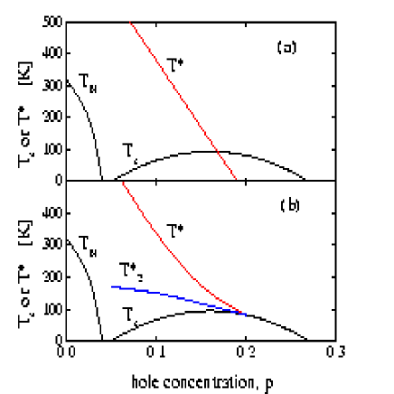
Figure 1: Two possible types of the phase diagram of HTSC – cuprates.

Depending on concentration of current carriers (in most cases holes) in highly conducting $CuO_{2}$ plane a number of phases is observed as well as regions with anomalous physical properties. For small concentration of holes all known HTSC – cuprates are antiferromagnetic insulators. As hole concentration grows Neel temperature $T_{N}$ drops rapidly from the values of the order of hundreds of $K$, becoming zero at hole concentration $p$ of the order of $0.05$ or even less, while the system becomes metallic (though this metal is rather bad). With the further growth of hole concentration the system becomes superconducting and superconducting critical temperature at first grows with hole concentration, becoming maximal at $p_{0}\approx 0.15-0.17$ (optimal doping), then drops to zero at $p\approx 0.25-0.30$, while in this (overdoped) region the metallic behavior persists. Metallic properties in the region of $p>p_{0}$ are more or less traditional (Fermi - liquid), while for $p<p_{0}$ the system is a kind of anomalous metal, not described (in the opinion of majority researchers) by Fermi - liquid theory.

Anomalies of physical properties which are attributed to the appearance of the pseudogap state are observed in metallic phase for $p<p_{0}$ and temperatures $T<T^{*}$, where $T^{*}$ falls from temperatures of the order of $T_{N}$ for $p\sim 0.05$, becoming zero at some “critical” concentration $p_{c}$, which is may be slightly larger than $p_{0}$ (Fig.1(a)), e.g. according to Ref.TL this happens at $p=p_{c}\approx 0.19$. In the opinion of a number of authors (mainly supporters of superconducting scenario of pseudogap formation) $T^{*}$ gradually approaches the line of superconducting $T_{c}$ close to the optimal concentration $p_{0}$ (Fig.1(b)). Below we shall see that the majority of new experimental data apparently confirm the type of the phase diagram shown in Fig.1(a) (see details in Ref. TL ). It should be stressed that temperature $T^{*}$, in the opinion of majority of researchers, does not have the meaning of a temperature of some kind of phase transition. It only determines some characteristic temperature scale below which the pseudogap anomalies appear in different measurements. Any kind of singularities of thermodynamic characteristics in this region of phase diagram are just absent . The general statement is that all these anomalies can be related to some drop (in this region) in the density of single – particle excitations close to the Fermi level, which corresponds to a general concept of the pseudogap . In this case the value of $T^{*}$ is just proportional to energy width of the pseudogap. Sometimes an additional temperature scale $T^{*}_{2}$ is also introduced, as shown in Fig. 1(b), attributed to a crossover from “weak” to “strong” pseudogap regime Sch , usually referring to some change in spin system response in the vicinity of this temperature. In the following we shall not be dealing with these details.

Now let us describe the most typical experimental signatures of pseudogap anomalies in HTSC – cuprates.

II.1 Specific Heat and Tunneling.

Consider first the data on electronic specific heat of HTSC – cuprates. In metals this contribution is usually represented as $C=\gamma(T)T$, so that in the normal state ($T>T_{c}$) $\gamma\sim N(0)$, where $N(0)$ – is the density of states at the Fermi level. For $T=T_{c}$ we have the well known anomaly due the second order transition and the value of $\gamma(T)$ acquires the characteristic peak (“jump” or discontinuity). As an example in Fig.2 we show some typical data obtained for $Y_{0.8}Ca_{0.2}Ba_{2}Cu_{3}O_{7-\delta}$ with different values of $\delta$ Loram .

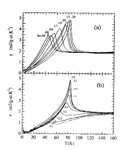
Figure 2: Electronic specific heat coefficient $\gamma$ in overdoped (a) and underdoped (b) $Y_{0.8}Ca_{0.2}Ba_{2}Cu_{3}O_{7-\delta}$ Loram .

In optimally doped and overdoped samples $\gamma(T)$ remains practically constant for all $T>T_{c}$, while for underdoped samples a significant drop of $\gamma(T)$ is observed for temperatures $T<150-200K$. This observation directly signifies to the drop in the electronic density of states at the Fermi level and formation of the pseudogap for $T<T^{*}$.

Note also that the value of the “jump” of specific heat at $T_{c}$ is much reduced as we go into the underdoped region. More detailed analysis TL shows that the appropriate value of $\Delta\gamma_{c}$ drops rather sharply, starting from the “critical” concentration of carriers $p_{c}\approx 0.19$, which is considered to be the point of appearance of the pseudogap in electronic spectrum.

Using more or less traditional expressions of BCS theory, specific heat data can be used to estimate the value of superconducting energy gap in electronic spectrum and its temperature dependence. In Fig.3 we show the data of Ref.Lor , obtained for $YBa_{2}Cu_{3}O_{7-\delta}$ ($YBCO$). It is seen that thus defined energy gap does not go to zero for $T=T_{c}$ (as it should be in a traditional superconductor) and there is a significant “tail” in the region of higher temperatures. This effect is stronger for more underdoped samples.

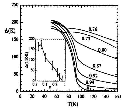
Figure 3: Temperature dependence of the energy gap for samples of $YBa_{2}Cu_{3}O_{6+x}$ with different compositions, determined from specific heat measurements Lor . The number at different curves denote the appropriate values of oxygen content $x$.

Often these data are naively interpreted as signifying Cooper pair formation at temperatures $T>T_{c}$.

Pseudogap formation is clearly seen in the experiments on single particle tunneling. In a widely cited Ref.Renn tunneling measurements were performed on single crystals of $Bi_{2}Sr_{2}CaCu_{2}O_{8+\delta}$ ($Bi-2212$) with different oxygen content. For underdoped samples the pseudogap formation in the density of states was clearly observed for temperatures higher than $T_{c}$. This pseudogap smoothly evolved into superconducting gap for $T<T_{c}$, which again was seen by many as a direct confirmation of superconducting nature of the pseudogap. Some signs of pseudogap existence was observed in this work also for slightly overdoped samples.

While discussing tunneling experiments in HTSC – cuprates, there is always a question of the surface quality of the samples. Thus, especially interesting the recent studies of Refs. Kras1 ; Kras2 , where an intrinsic tunneling was measured on the so called mesa – structures , specially formed (by microlitography) on the surface of the same system $Bi-2212$. These experiments clearly demonstrated the existence of superconducting gap approaching zero at $T=T_{c}$ on the background of smooth pseudogap, which exists at higher temperatures. The appropriate tunneling date are shown in Fig.4. Typical peaks due to superconducting gap opening are seen on the background of smooth minimum in the density of states due to pseudogap.

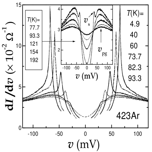
Figure 4: Differential conductance of nearly optimally doped $Bi-2212$ for different temperatures. At the insert – results for higher $T$ Kras1 .

It is especially important that in Ref.Kras2 it was demonstrated that superconducting peculiarities of tunneling characteristics were destroyed by the external magnetic field, while the pseudogap remained practically independent of the field strength, which clearly shows its non – superconducting nature. Appropriate data are shown in Fig.5

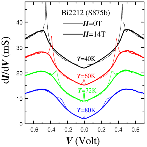
Figure 5: Differential conductance of nearly optimally doped $Bi-2212$ for different temperatures in magnetic field $H=0$ (thin lines) and for $H=14T$ (thick lines) Kras2 .

II.2 NMR and Transport Properties.

Formation of the pseudogap signals itself also in transport properties of HTSC – systems in normal state, Knight shift and NMR – relaxation. In particular it is thought to be a reason for the change of the standard (for optimally doped samples) linear temperature dependence of resistivity in the region of $T<T^{*}$ for underdoped samples. The value of the Knight shift in underdoped samples becomes temperature dependent – for $T<T^{*}$ it drops rather rapidly. Analogous behavior is observed in underdoped region for the value of $(TT_{1})^{-1}$, where $T_{1}$ – is NMR relaxation time. Let us remind that in usual metals the Knight shift is proportional to $N(0)$, while $(TT_{1})^{-1}\sim N^{2}(0)$ (Korringa relation). Resistivity $\rho$ is usually proportional to the scattering rate (inverse mean – free time) $\gamma\sim N(0)$. Thus, the notable suppression of these characteristics is naturally explained by the drop in the density of states $N(0)$ at the Fermi level. Note that this interpretation is obviously oversimplified, moreover when we discuss the temperature dependence of these physical characteristics. For example, in the case of resistivity this dependence is usually mainly determined by inelastic scattering processes and the physical mechanism of these in HTSC – cuprates is still far from being clear. The drop in the density of states, interpreted as partial dielectrization of electronic spectrum, may also lead to the appropriate growth of resistivity.

In Fig.6 taken from Ref.BatlVar we show the summary of experimental data for underdoped samples of $YBa_{2}Cu_{4}O_{8}$ using the results of Refs.Buch ; Yas ; All .

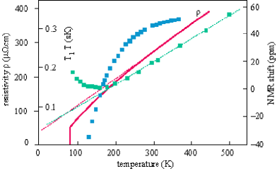
Figure 6: Influence of the pseudogap formation on resistivity, Knight shift and NMR relaxation in underdoped $YBa_{2}Cu_{4}O_{8}$. The changes in temperature dependences in the region of $T<200-300K$ is attributed to pseudogap formation in the density of states BatlVar .

In Fig.7 we show the data of Ref.Gorn on the measurements of $(TT_{1})^{-1}$ on ${}^{63}Cu$-nuclei in slightly underdoped $YBa_{2}Cu_{3}O_{7-\delta}$ in strong enough magnetic field.

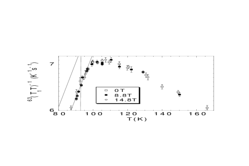
Figure 7: NMR relaxation rate $(TT_{1})^{-1}$ for slightly underdoped $YBa_{2}Cu_{3}O_{7-\delta}$ in strong magnetic field, directed along the $c$-axis of the sample Gorn . Vertical line shows $T_{c}$ in zero field . The straight line parallel to the data estimates the expected shift of data in the case of pseudogap suppression by magnetic field, its position is determined by the observed shift of $T_{c}$.

It is seen that the magnetic field dependence of the data is practically absent, giving the strong support for non - superconducting nature of the pseudogap, as in the opposite case magnetic field should significantly change the size of the effect. Note that the expected influence of magnetic field upon the Knight shift and NMR relaxation of ${}^{63}Cu$ was observed in slightly overdoped $TlSr_{2}CaCu_{2}O_{6.8}$ where it was accurately described by the effects of suppression of superconducting fluctuations Guo . This fact can be seen as an evidence of disappearance of the pseudogap of non - superconducting nature (independent of magnetic field) at some lower concentration of current carriers.

Let us stress that in different experiments the characteristic temperature $T^{*}$ below which the anomalies attributed to pseudogap appear can somehow change depending on the quantity being measured. However, in most cases there is a systematic dependence of $T^{*}$ on doping and this temperature tends to zero close to optimal concentration of current carriers or at slightly higher concentrations.

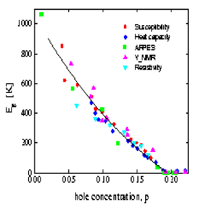
Figure 8: Dependence of energy scale characterizing the width of the pseudogap $E_{g}$ in $YBCO$ on concentration of holes following from different experiments TL .

It is clear that $T^{*}$ does not represent any strictly defined temperature (e.g. of some phase transition) but only determines some characteristic crossover temperature (energy) scale below which pseudogap anomalies appear . This energy scale may be determined from experimental data using some rough model of the energy dependence of the density of states close to the Fermi level within the pseudogap region (e.g. triangular with the width of $E_{g}$, giving $T^{*}=0.4E_{g}$) TL . In Fig.8 we present the summary of the values of pseudogap width determined in this way from different experiments on $YBCO$ for different hole concentrations TL . It is seen that the pseudogap “closes” at some critical value of $p_{c}\approx 0.19$. Once again let us stress that both the line of $T^{*}$ on the phase diagram and “critical” concentration $p_{c}$ apparently possess only qualitative meaning. However, there are also attempts to interpret $p_{c}$ as some kind of a “quantum” critical point TaLor .

II.3 Optical Conductivity.

Pseudogap formation in underdoped HTSC – cuprates is also clearly seen in numerous measurements of optical conductivity, both for electric field vector polarized along the highly conducting $CuO_{2}$ plane and along orthogonal direction of tetragonal axis $c$. These experiments are reviewed in detail in Ref.Tim ; PBT . As a typical example in Fig.9 we show the data of Ref.STP on optical conductivity in the $CuO_{2}$ - plane of underdoped $La_{1.87}Sr_{0.13}CuO_{4}$.

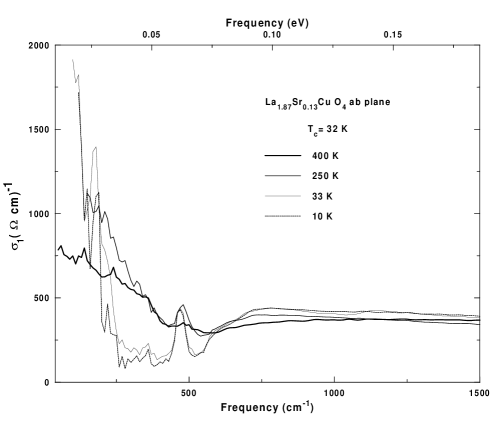
Figure 9: Real part of optical conductivity in $ab$ - plane of $La_{1.87}Sr_{0.13}CuO_{4}$ for different temperatures STP .

Characteristic feature of these data is the presence of rather narrow “Drude - like” peak in the frequency region $\omega<250cm^{-1}$ and the appearance of “pseudogap suppression” of conductivity in the interval of $250-700cm^{-1}$ accompanied by smooth maximum around $\omega\sim 800cm^{-1}$. Especially sharply pseudogap anomalies are seen after the experimental data are expressed in terms of the so called generalized Drude formula Tim ; PBT , which introduces the effective (frequency dependent) scattering rate and effective mass of current carriers:

$$\frac{1}{\tau(\omega)}=\frac{\omega_{p}^{2}}{4\pi}Re\left(\frac{1}{\sigma(\omega)}\right)$$ (1)

$$\frac{m^{*}(\omega)}{m}=\frac{1}{\omega}\frac{\omega^{2}_{p}}{4\pi}Im\left(\frac{1}{\sigma(\omega)}\right)$$ (2)

where $\sigma(\omega)$ – the observed complex conductivity, $\omega_{p}$ – plasma frequency, $m$ – mass of the free electron. Note that the use of expressions (1), (2) is just another form of expression of the same experimental data in the form of $1/\tau(\omega)$ and $m^{*}(\omega)$ instead of two more usual characteristics — the real and imaginary parts of conductivity. Accordingly there is no especially deep physical meaning in both $\tau(\omega)$ and $m^{*}(\omega)$. However, this form of presentation of experimental data in optics is widely used in the literature.

In Fig.10 we present the results of such a representation of experimental data of the sort shown in Fig.9 STP .

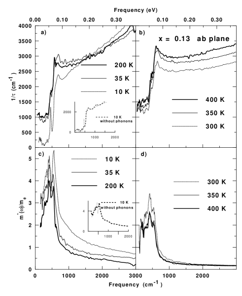
Figure 10: Generalized scattering rate and effective mass as functions of the frequency of the external field obtained from the fit of optical data for $La_{1.87}Sr_{0.13}CuO_{4}$ to generalized Drude formula STP : (a), (c) – for temperatures $T<250K$, when the linear growth of $1/\tau$ with frequency is observed for $\omega>700cm^{-1}$, (b), (d) – higher temperatures, when the linear growth of $1/\tau$ is practically invisible.

It is seen that the effective scattering rate for temperatures less than $T^{*}\sim 450K$ is sharply suppressed for frequencies of an external field less than $700cm^{-1}$, while for higher frequencies $\frac{1}{\tau(\omega)}$ grows linearly with $\omega$, demonstrating the anomalous non - Fermi liquid behavior. The presence of this dip in $1/\tau(\omega)$ is most vivid reflection of the pseudogap in optical data. At the same time we have to note that the frequency dependence of $m^{*}(\omega)$ shown in Fig.10 apparently has no clear interpretation.

Analogous behavior of $1/\tau(\omega)$ is also observed in data on transverse optical conductivity $\sigma_{c}(\omega)$, practically for all HTSC – cuprates studied in underdoped region Tim ; PBT .

II.4 Fermi Surface and ARPES.

Especially spectacular effects due to formation of the pseudogap are observed in experiments on angle – resolved photoemission (ARPES) RC ; TM . This method is, first of all, decisive in studies of the topology of the Fermi surface of HTSC – cuprates Dessau ; Shen ; RC , being practically the sole source of this information.

In Fig.11 we show the data of Ref.Ino on the Fermi surface of $La_{2-x}Sr_{x}CuO_{4}$ for two different compositions. In overdoped state $(x=0.3)$ Fermi surface is electronic and centered around the point $\Gamma(0,0)$ in Brillouin zone. As concentration $x$ diminishes the topology of the Fermi surface changes, so that for optimal concentration of $Sr$ and in underdoped region $(x=0.1)$ it becomes hole - like and centered around the point $Y(\pi,\pi)$. Precisely this topology is observed in majority of ARPES – experiments for almost all HTSC – cuprates.

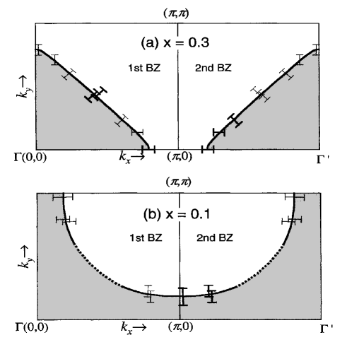
Figure 11: Fermi surface of $La_{2-x}Sr_{x}CuO_{4}$ for overdoped (a) and underdoped (b) cases Ino .

As an interesting example in Fig.12 from Ref.Onell we show the hole - like Fermi surface of most extensively studied (by ARPES) system $Bi-2212$ in overdoped state. The spectacular feature here is the observation of large flat parts of the Fermi surface, orthogonal to direction $YM$ and symmetric directions. Independently this result was confirmed in Ref.ZX for optimally doped system. The presence of the flat parts (patches) on the Fermi surface may be very important for the construction of microscopic theories of electronic properties of HTSC – systems.

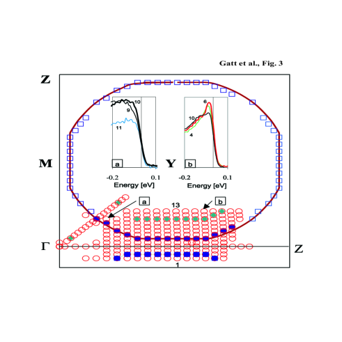
Figure 12: Fermi surface of overdoped $Bi-2212$ Onell . Circles represent points where measurements were performed. At the inserts – energy distribution of photoelectrons along the directions $a$ and $b$, shown by arrows.

Dropping these fine details in the first rough enough approximation the observed topology of the Fermi surface and the spectrum of elementary excitations in the $CuO_{2}$ plane can be rather accurately described by the tight - binding model:

$$\varepsilon_{\bf k}=-2t(\cos k_{x}a+\cos k_{y}a)-4t^{\prime}\cos k_{x}a\cos k_{y}a$$ (3)

where $t\approx 0.25eV$ – transfer integral between nearest neighbors, and $t^{\prime}$ – transfer integral between second nearest neighbors, which may change between $t^{\prime}\approx-0.45t$ for $YBa_{2}Cu_{3}O_{7-\delta}$ and $t^{\prime}\approx-0.25t$ for $La_{2-x}Sr_{x}CuO_{4}$, $a$ – lattice constant.

Quite recently the simple picture described above was seriously revised in Refs.ZX ; Chu ; Gr ; Bog using the new ARPES data obtained with synchrotron radiation of higher energy, than in previous experiments. It was claimed that the Fermi surface of $Bi-2212$ is electronic and centered around point $\Gamma$. The main discrepancies with previous data are in the most interesting (for us) vicinity of the point $(0,\pi)$ in the inverse space. These claims, however, were met with sharp objections from other groups of ARPES experimentalists Fr ; Mes ; Ban ; Bor ; Leg . The question remains open, but in the following we shall adhere to traditional interpretation.

There are several good reviews on the observation of pseudogap anomalies in ARPES experiments R ; RC ; TM , so below we shall limit ourselves only to basic qualitative statements. The intensity of ARPES (energy distribution of photoelectrons) in fact is determined as RC :

$$I({\bf k}\omega)=I_{0}({\bf k})f(\omega)A({\bf k}\omega)$$ (4)

where $\bf k$ – is the electron momentum in the Brillouin zone, $\omega$ – the energy of initial state with respect to the Fermi level (chemical potential), $I_{0}({\bf k})$ includes kinematic factors and the square of the matrix element of electron – photon interaction (and in rough enough approximation can be considered a constant). The value

$$A({\bf k},\omega)=-\frac{1}{\pi}ImG({\bf k},\omega+i\delta)$$ (5)

where $G({\bf k},\omega)$ – is the Green’s function, represents the spectral density of electrons. Fermi distribution $f(\omega)=[exp(\omega/T)+1]^{-1}$ reflects the fact that only electrons from the occupied states participate in photoemission. Thus in a rough approximation we may say that ARPES experiments directly measure the product of $f(\omega)A({\bf k}\omega)$, and we can get the direct information on the spectral properties of single - particle excitations in our system.

In Fig.13 we show typical ARPES data for $Bi_{2}Sr_{2}CaCu_{2}O_{8}$ Norm , measured in three different points on the Fermi surface for different temperatures.

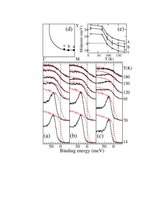
Figure 13: ARPES spectra in three different points $a,b,c$ on the Fermi surface of $Bi-2212$ for underdoped sample with $T_{c}=85K$. Thin lines – ARPES spectrum of a reference sample of $Pt$ Norm .

The appearance of the gap (pseudogap) is reflected in the shift (to the left) of the leading edge of photoelectron energy distribution curve, compared to the reference spectrum of a good metal $(Pt)$. It is seen that the gap is closed at different temperatures for for different values of ${\bf k}$, while its width diminishes as we move away from $(0,0)-(0,\pi)$ direction. Pseudogap is completely absent in the direction of the zone diagonal $(0,0)-(\pi,\pi)$. At low temperatures these data are consistent with the picture of $d$-wave pairing, which is well established from numerous experiments on HTSC – cuprates Legg ; Iz . It is important, however, that this “gap” in ARPES data is observed also for temperatures significantly higher than the temperature of superconducting transition $T_{c}$.

In Fig.14 we show the angular dependence of the gap width in the Brillouin zone and the temperature dependence of its maximum value for the number of samples of $Bi-2212$ with different oxygen content, obtained via ARPES in Ref.Din . It is seen that with the general $d$-wave symmetry, the gap in the spectrum of optimally doped system becomes zero practically at $T=T_{c}$, while for underdoped samples there appear characteristic “tails” in the temperature dependence of the gap for $T>T_{c}$, quite similar to those shown in Fig.3. Qualitatively we may say that the formation of anisotropic (in reciprocal space) pseudogap for $T>T_{c}$, continuously evolving into superconducting gap for $T<T_{c}$, leads to a “destruction” of the parts of the Fermi surface of underdoped samples already for $T<T^{*}$ and around the point $(0,\pi)$ (and symmetric to it), and that the effective width of these parts grows as the temperature is lowered Nrm .

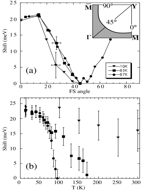
Figure 14: Angular (a) and temperature (b) dependence of energy gap in $Bi-2212$, obtained from ARPES data Nrm for samples with $T_{c}=87K$ (nearly optimally doped), $T_{c}=83K$ and $T_{c}=10K$ (underdoped).

Central point is, of course, the evolution of spectral density $A({\bf k}_{F},\omega)$ at the Fermi surface. Under rather plausible assumptions this may be directly obtained from ARPES data Nrm . In case of electron - hole symmetry we have $A({\bf k}_{F},\omega)=A({\bf k}_{F},-\omega)$ (which is always valid close enough to the Fermi level, in real systems for $|\omega|$ less than few tenths of $meV$), so that, with the account of $f(-\omega)=1-f(-\omega)$, from (4) for ${\bf k}={\bf k}_{F}$ we immediately get $I(\omega)+I(-\omega)=A({\bf k}_{F},\omega)$. Thus, the spectral density at the Fermi surface may be obtained directly from experiments, more precisely from the symmetrized ARPES - spectrum $I(\omega)+I(-\omega)$. As an example of such approach, in Fig.15 we present the data of Ref.NorRan for underdoped sample of $Bi-2212$ with $T_{c}=83K$ and overdoped sample with $T_{c}=82K$ for different temperatures. It is seen that the existence of the pseudogap is reflected in typical two - peak structure of the spectral density, appearing for the underdoped system at temperatures significantly higher than $T_{c}$.

Figure 15: Symmetrized ARPES spectra for overdoped sample of $Bi-2212$ with $T_{c}=82K$ (a) and underdoped sample with $T_{c}=83K$ (b) at the point of intersection of the Fermi surface with Brillouin zone border $(0,\pi)-(\pi,\pi)$ NorRan .

Let us stress that well defined quasiparticles correspond to sharp enough peak of the spectral density $A({\bf k}_{F},\omega)$ at $\omega=0$. This type of behavior is practically unobservable in HTSC – cuprates, at least for $T>T_{c}$. In principle, this does not seem surprising – it is rather difficult to imagine well defined quasiparticles almost in any system for $T>100K$! However, the much improved resolution of modern ARPES installations apparently allows to conclude, that the actual width of the peak observed is larger than experimental resolution, so that the problem can be studied experimentally Kami . It appears that in superconducting state, for $T\ll T_{c}$, in the vicinity of the crossing of the Fermi surface with the diagonal of the Brillouin zone ($(0,0)-(\pi,\pi)$ direction), there appears sharp enough peak of the spectral density, corresponding to well defined quasiparticles Kami . However in the vicinity of the point $(0,\pi)$ the Fermi surface is “destroyed” by superconducting gap, corresponding to $d$-wave pairing, which leads to the two - peak structure of the spectral density.

The smooth evolution of ARPES pseudogap observed for $T>T_{c}$ into superconducting gap corresponding to $d$-wave pairing for $T<T_{c}$ is often considered as an evidence of superconducting nature of the pseudogap. However, most probably this is wrong. In this respect we should like to note the very interesting paper Ronn , where the ARPES measurements were performed on dielectric oxide $Ca_{2}CuO_{2}Cl_{2}$, which is structurally analogous to $La_{2}CuO_{4}$ and becomes a high – temperature superconductor after doping by $Na$ or $K$. ARPES measurements on this system were possible in insulating phase due to especially good quality of the sample surface. The exciting discovery made in Ref.Ronn was apparently first observation of the “remnant” Fermi surface in this Mott dielectric, which is everywhere “closed” by the gap (apparently of the Mott – Hubbard nature). At the same time a strong anisotropy of this gap in inverse space with the symmetry of $d$-wave type was also observed Ronn , very similar to analogous data for HTSC – systems in metallic phase. It seems plausible that this anisotropic gap has the same nature as high - energy pseudogap say in $Bi-2212$ Ronn . Of course, it is quite clear that there is no any kind of Cooper pairing in this insulator.

II.5 Other Experiments.

Pseudogap behavior is also observed in a number of other experiments, such as electronic Raman scattering Hack and magnetic scattering of neutrons Bourg . All these experiments are interpreted as an evidence for significant suppression of the single - particle density of states close to the Fermi level of underdoped HTSC - cuprates for temperatures $T<T^{*}$, that is already in normal phase. Due to a space shortage we shall not discuss these data in any detail, moreover that a good review of these can be found in papers cited above, as well as in Ref.Tim .

III Theoretical Models of Pseudogap State.

III.1 Scattering by Fluctuations of Short - Range Order: Qualitative Picture.

As was already noted above there exist two main theoretical scenario to explain pseudogap anomalies of HTSC – systems. The first is based on the model of Cooper pair formation above the temperature of superconducting transition (precursor pairing), while the second assumes that formation of the pseudogap state is due to fluctuations of short - range order of “dielectric” type (e.g. antiferromagnetic or charge density wave) existing in the underdoped region of the phase diagram and leading to strong scattering of electrons and pseudogap renormalization of the spectrum. This second scenario seems more preferable both because of experimental evidence , described above, and due to the simple fact that all pseudogap anomalies become stronger for stronger underdoping, when system moves from optimal (for superconductivity) composition towards insulating (antiferromagnetic) region on the phase diagram.

Consider typical Fermi surface of current carriers in $CuO_{2}$ plane, shown in Fig.16. Phase transition to antiferromagnetic state leads to doubling of lattice period and appearance of “magnetic” Brillouin zone in reciprocal space, shown by dashed lines in Fig.16 . If the energy spectrum of current carriers is given by (3) with $t^{\prime}=0$, then for the case of half - filled band the Fermi surface is just a square coinciding borders of magnetic zone and there is complete nesting — flat parts of the Fermi surface coincide after translation by vector of antiferromagnetism ${\bf Q}=(\pm\pi/a,\pm\pi/a)$. For $T=0$ electronic spectrum is unstable — energy gap is opened everywhere at the Fermi surface and the system becomes insulator due to formation of antiferromagnetic spin density wave (SDW) These arguments lay behind the popular explanation of antiferromagnetism of HTSC – cuprates, let us quote e.g. Ref.SWZ . The review of this and similar models can be found in Izy .

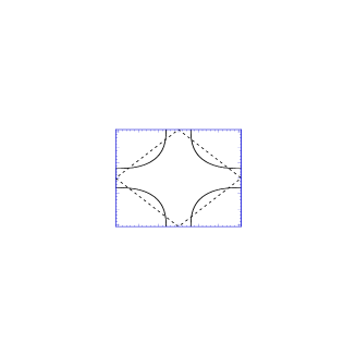
Figure 16: Fermi surface in the Brillouin zone and “hot spots” model. Dashed lines represent borders of magnetic Brillouin zone appearing after period doubling due to appearance of antiferromagnetic long - range order. “Hot spots” are defined as points of crossing of the Fermi surface with borders of magnetic zone.

In the case of the Fermi surface shown in Fig.16 the appearance of antiferromagnetic long - range order, in accordance with general rules of the band theory Zim , leads to the appearance of discontinuities of isoenergetic surfaces (e.g. Fermi surface) at crossing points with borders of new (magnetic) Brillouin zone due to gap opening at points connected by vector ${\bf Q}$.

In the most part of underdoped region of the phase diagram of HTSC – cuprates there is no antiferromagnetic long - range order, however quite a number of experiments indicates the existence (below the $T^{*}$ line) of well developed fluctuations of antiferromagnetic short - range order. In the model of “nearly antiferromagnetic” Fermi liquid Mont1 ; Mont2 an effective interaction of electrons with spin fluctuations is described by dynamic spin susceptibility $\chi_{\bf q}(\omega)$, which can be written in the following form determined from the fit to NMR experiments MilMon ; Iz :

$$V_{eff}({\bf q},\omega)=g^{2}\chi_{\bf q}(\omega)\approx\frac{g^{2}\xi^{2}}{1+\xi^{2}({\bf q-Q})^{2}-i\frac{\omega}{\omega_{sf}}}$$ (6)

where $g$ – is the coupling constant, $\xi$ – correlation length of spin fluctuations (short - range order), ${\bf Q}=(\pm\pi/a,\pm\pi/a)$ – vector of antiferromagnetic ordering in insulating phase, $\omega_{sf}$ – characteristic frequency of spin fluctuations.

Due to the fact that dynamic spin susceptibility $\chi_{\bf q}(\omega)$ possesses peaks at wave vectors smeared around $(\pm\pi/a,\pm\pi/a)$, there appear “two types” of quasiparticles – “hot quasiparticles” with momenta from the vicinity of “hot spots” at the Fermi surface (Fig.16) and with energies satisfying the following inequality ($v_{F}$ – velocity at the Fermi surface):

$$|\varepsilon_{\bf k}-\varepsilon_{\bf k+Q}|<v_{F}/\xi,$$ (7)

and “cold” ones, with momenta close to the parts of the Fermi surface around Brillouin zone diagonals $|p_{x}|=|p_{y}|$ and not satisfying (7) Sch . This terminology is due to the fact that quasiparticles from the vicinity of “hot spots” are strongly scattered with momentum transfer of the order of ${\bf Q}$, because of strong interaction with spin fluctuations (6), while for quasiparticles with momenta far from “hot spots” this interaction is much weaker. In the following this model will be called “hot spot” model.

Correlation length of short - range order fluctuations $\xi$, defined in (6), is very important for the following discussion. Note that in real HTSC – systems it is usually not very large and changes in the interval of $2a<\xi<8a$ BarzP ; P97 .

Characteristic frequency of spin fluctuations $\omega_{sf}$, depending on the compound and doping, is usually in the interval of $10-100K$ BarzP ; P97 , so that in most part of pseudogap region on the phase diagram we can satisfy an inequality $\pi T\gg\omega_{sf}$, which allows us to neglect spin dynamics and use quasistatic approximation:

$$V_{eff}({\bf q})=\tilde{W}^{2}\frac{\xi^{2}}{1+\xi^{2}({\bf q-Q})^{2}}$$ (8)

where $\tilde{W}$ – is an effective parameter of dimensions of energy, which in the model of AFM fluctuations can be written as Sch :

$$\tilde{W}^{2}=g^{2}T\sum_{m{\bf q}}\chi_{\bf q}(i\omega_{m})=g^{2}<{\bf S}_{i}^{2}>/3$$ (9)

where ${\bf S}_{i}$ is the spin on the lattice site (ion of $Cu$ in the $CuO_{2}$ plane of HTSC – cuprates).

In the following we shall consider both $\tilde{W}$ and $\xi$ as phenomenological parameters. In particular, the value of $\tilde{W}$ determines effective width of the pseudogap. The full microscopic theory of the pseudogap state will not be our aim, we shall only try to model the appropriate renormalization of electronic spectrum and its influence on physical properties, e.g. superconductivity.

Significant simplification of calculations appears if instead of (8) we use the model interaction of the form (similar simplification was first used in Ref.Kam ):

$$V_{eff}({\bf q})=W^{2}\frac{2\xi^{-1}}{\xi^{-2}+(q_{x}-Q_{x})^{2}}\frac{2\xi^{-1}}{\xi^{-2}+(q_{y}-Q_{y})^{2}}$$ (10)

where $W^{2}=\tilde{W}^{2}/4$. In fact (10) is qualitatively quite similar to (8) and differs from it only slightly quantitatively in most interesting region of $|{\bf q-Q}|<\xi^{-1}$. Analogous but a little bit different form of effective interaction was used in Ref.Sch . In this way we achieve effectively one - dimensional situation.

Scattering by AFM fluctuations in HTSC – cuprates is not always most intensive at vector ${\bf Q}=(\pi/a,\pi/a)$ commensurate with the inverse lattice vectors, in general case vector ${\bf Q}$ may correspond to incommensurate scattering. Keeping in mind the observed topology of the Fermi surface with flat parts (patches) as shown in Fig.12, we may propose another model for scattering by fluctuations of AFM short - range order , which we shall call the “hot patches” model PS . Assume that the Fermi surface of our two - dimensional system of electrons has the form, shown in Fig.17. The size of “hot patch” is determined by the angular parameter $\alpha$. It is well known that the presence of flat parts on the Fermi surface leads to instabilities either of charge density wave (CDW) or spin density wave (SDW) type, with the establishment of the appropriate long - range order and opening of (dielectric) energy gap on these parts of the Fermi surface. Here we are interested in situation typical of fluctuation region of the appropriate phase transition, when there is still no long - range order present . Similar model of the Fermi surface was introduced a number of years ago as a possible model for HTSC – cuprates in Refs.Vir ; Ruv ; Dz , where rather detailed analysis of microscopic criteria for the appearance of antiferromagnetic and superconducting phases on the phase diagram was performed.

Figure 17: Fermi surface in the model of “hot patches”, which are shown by thick lines (e.g. of the width of $\sim\xi^{-1}$). The angle $\alpha$ determines the size of a “hot patch” PS , $\alpha=\pi/4$ corresponds to the square Fermi surface.

Fluctuations of short - range order are assumed to be static and Gaussian and the appropriate correlation function is defined as (similar to Kam ):

$$S({\bf q})=\frac{1}{\pi^{2}}\frac{\xi^{-1}}{(q_{x}-Q_{x})^{2}+\xi^{-2}}\frac{\xi^{-1}}{(q_{y}-Q_{y})^{2}+\xi^{-2}}$$ (11)

Here $\xi$ – is again the correlation length of fluctuations, while the scattering vector is taken as $Q_{x}=\pm 2k_{F}$, $Q_{y}=0$ or $Q_{y}=\pm 2k_{F}$, $Q_{x}=0$. It is assumed that only electrons from flat (“hot”) parts of the Fermi surface shown in Fig.17 interact with these fluctuations and this scattering is in fact one - dimensional. For the special case of $\alpha=\pi/4$ we obtain square Fermi surface and the problem becomes strictly one - dimensional. For $\alpha<\pi/4$ there are also “cold” parts present at the Fermi surface and the scattering there is either absent or weak enough. Effective interaction of electrons from “hot” patches with fluctuations will be descibed by $(2\pi)^{2}W^{2}S({\bf q})$, where $W$ is the parameter with dimension of energy, defining again the energy scale (width) of the pseudogap. . The choice of scattering vector ${\bf Q}=(\pm 2k_{F},0)$ or ${\bf Q}=(0,\pm 2k_{F})$ assumes the picture of incommensurate fluctuations as the Fermi momentum $p_{F}=\hbar k_{F}$ is in general not connected with the inverse lattice period. Commensurate case can also be studied within this model PS .

The basic idea of models under discussion is the presence of strong scattering on fluctuations of short - range order, which, according to (6), (10) or (11), is effective in a limited region of inverse space with the width of the order of $\xi^{-1}$ around the “hot” spots or patches, and which leads to pseudogap – like renormalization of electronic spectrum in these regions.

Let us present a simple qualitative analysis of possible changes of single - electron spectral density (5). In the standard Fermi - liquid theory AGD the single - electron Green’s function for the metal can be written as:

$$G(\omega,{\bf k})=\frac{Z_{\bf k}}{\omega-\xi_{\bf k}-i\gamma_{\bf k}}+G_{incoh}$$ (12)

where $\xi_{\bf k}=\varepsilon_{\bf k}-\mu$ – is the quasiparticle energy with respect to the Fermi level (chemical potential) $\mu$, $\gamma_{\bf k}$ – its damping. The residue in the pole $0<Z_{\bf k}<1$, $G_{incoh}$ – non - singular contribution of many - particle excitations. Then the appropriate spectral density is:

$$A(\omega,{\bf k})=\frac{1}{\pi}Z_{\bf k}\frac{\gamma_{\bf k}}{(\omega-\xi_{\bf k})^{2}+\gamma^{2}_{\bf k}}+...$$ (13)

where dots denote more or less regular contribution due to $G_{incoh}$, while the quasiparticle spectrum is reflected in a narrow (as damping $\gamma_{\bf k}$ is small close to the Fermi level) Lorentzian peak. This situation is illustrated in Fig.18(a).

Figure 18: Qualitative evolution of the spectral density. (a) – normal metal (Fermi - liquid), $\xi_{\bf k}=0$ – at the Fermi surface. (b) – two narrow peaks corresponding to Bogoliubov’s quasiparticles in the system with dielectric gap $W_{\bf k}$ (CDW or SDW long - range order). Smeared maxima – system without long - range order (pseudogap behavior), $\xi_{\bf k}=0$ – at the Fermi surface. (c) The same as in (b), but for $\xi_{\bf k}>0$, i.e. above the Fermi surface. In this case a characteristic asymmetry of the spectral density appear.

If the long - range order of SDW or CDW type appears the spectrum of elementary excitations acquires the (dielectric) gap $W_{\bf k}$ (dependence on ${\bf k}$ stresses the possibility of gap opening on some part of the Fermi surface only) and single - electron Green’s function has the form of Gorkov’s function SWZ ; Izy , where we can add some damping $\Gamma_{\bf k}$:

$$G(\omega,{\bf k})=\frac{u^{2}_{\bf k}}{\omega-E_{\bf k}+i\Gamma_{\bf k}}+\frac{v^{2}_{\bf k}}{\omega+E_{\bf k}-i\Gamma_{\bf k}}$$ (14)

where the spectrum of elementary excitations:

$$E_{\bf k}=\sqrt{\xi^{2}_{\bf k}+W^{2}_{\bf k}}$$ (15)

and we introduced Bogoliubov’s coefficients:

$$u^{2}_{\bf k}=\frac{1}{2}\left(1+\frac{\xi_{\bf k}}{E_{\bf k}}\right)$$ (16)

$$v^{2}_{\bf k}=\frac{1}{2}\left(1-\frac{\xi_{\bf k}}{E_{\bf k}}\right)$$ (17)

Then the spectral density:

$$A(\omega{\bf k})=\frac{u^{2}_{\bf k}}{\pi}\frac{\Gamma_{\bf k}}{(\omega-E_{\bf k})^{2}+\Gamma^{2}_{\bf k}}+\frac{v^{2}_{\bf k}}{\pi}\frac{\Gamma_{\bf k}}{(\omega+E_{\bf k})^{2}+\Gamma^{2}_{\bf k}}+...$$ (18)

where now two peaks are present (both narrow if $\Gamma_{\bf k}$ is small), corresponding to Bogoliubov’s quasiparticles.

Let us now consider the situation when SDW or CDW long - range order is absent, but there is a strong scattering on fluctuations of short - range order with appropriate wave vectors (cf. (6),(10) or (11)). Then it is not difficult to imagine that in the spectral density remains some “reminiscence” (or “anticipation”) of dielectric energy gap opening (in the same region of momentum space) in the form of characteristic smeared two - peak structure, as shown in Fig.18 . The width of both maxima, naturally, is determined by some parameter like $v_{F}/\xi$, i.e. by inverse time of flight of an electron through the region of the typical size of $\xi$, where effectively persists “dielectric” ordering. It is seen that this qualitative picture is quite similar to ARPES data shown in Fig.15. Below we shall see that more rigorous analysis leads just to the same conclusions. Further parts of the review will be dealing with justification of this qualitative picture and some of its consequences.

III.2 Recurrence Relations for the Green’s Functions.

The model of the pseudogap state which will be discussed below is, in fact, a two - dimensional generalization of the model proposed many years ago for pseudogap formation in fluctuation region of Peierls (CDW) structural transition in one - dimensional systems LRA ; C1 ; C2 ; C79 . In Refs.C1 ; C2 we obtained an exact solution of this model in the limit of very large correlation lengths of fluctuations of short - range order $\xi\to\infty$, while in Ref.C79 we proposed the appropriate generalization for the case of finite $\xi$. The main advantage of these results, in comparison with Ref.LRA , was the complete account of all Feynman diagrams of perturbation series for electron interaction with fluctuations of short - range order. Appropriate two - dimensional generalization of this approach was made in Refs.Sch ; KS for “hot spots” model, while for “hot patches” model it can be done directly due to effective one - dimensionality of this model.

Contribution of an arbitrary diagram for electron self - energy of single - particle Green’s function in the $N$-th order of perturbation theory over interaction with fluctuations, given by (10) or (11), can be approximately written in the following form KS :

$$\Sigma^{(N)}(\varepsilon_{n}{\bf p})=W^{2N}\prod_{j=1}^{2N-1}\frac{1}{i\varepsilon_{n}-\xi_{j}+in_{j}v_{j}\kappa}$$ (19)

where for the “hot spots” model $\xi_{j}=\xi_{\bf p+Q}$ and $v_{j}=|v_{\bf p+Q}^{x}|+|v_{\bf p+Q}^{y}|$ for odd $j$ and $\xi_{j}=\xi_{\bf p}$ and $v_{j}=|v_{\bf p}^{x}|+|v_{\bf p}^{y}|$ for even $j$. In the “hot patches” model $\xi_{j}=(-1)^{j}\xi_{\bf p}$, $v_{j}=v_{F}$. In (19) we have introduced an inverse correlation length $\kappa=\xi^{-1}$, $n_{j}$ – is the number of interaction lines, surrounding $j$-th (from the beginning) Green’s function in a given diagram, $\varepsilon_{n}=(2n+1)\pi T$ and, for definiteness, $\varepsilon_{n}>0$.

As a matter of fact, expression (19) constitutes rather successful Ansatz, which allows to calculate the contribution of an arbitrary diagram in any order. In this case any diagram with intersections of interaction lines is actually equal to some specific diagram of the same order without intersecting interaction lines. Thus, in fact we may consider only diagrams without intersections of interaction lines, taking those with intersections into account by additional combinatorial factors, associated with interaction lines. This approach was first used (for another problem) by Elyutin Ely and applied to one - dimensional model of the pseudogap state in Ref.C79 . Actually, Ansatz (19) is not exact Tchern , but it may be justified in two - dimensional case for certain topologies of the Fermi surface, such that electron velocity components in “hot spots” connected by vector ${\bf Q}$ have the same sign, so that $v_{\bf p}^{x}v_{\bf p+Q}^{x}>0$ and $v_{\bf p}^{y}v_{\bf p+Q}^{y}>0$ KS . This condition is not satisfied in one - dimensional case and also for topologies of Fermi surfaces typical for HTSC – cuprates, as shown in Fig.16. However, in Ref.KS it was shown that even in these cases the use of (19) gives quite satisfactory results and reproduce the exactly known limits of $\xi\to\infty$ and $\xi\to 0$ .

As a result we obtain the following recursion relation for one - electron Green’s function (continuous chain approximation C79 ):

$$G^{-1}(\varepsilon_{n}\xi_{\bf p})=G_{0}^{-1}(\varepsilon_{n}\xi_{\bf p})-\Sigma_{1}(\varepsilon_{n}\xi_{\bf p})$$ (20)

$$\Sigma_{k}(\varepsilon_{n}\xi_{\bf p})=W^{2}\frac{v(k)}{i\varepsilon_{n}-\xi_{k}+ikv_{k}\kappa-\Sigma_{k+1}(\varepsilon_{n}\xi_{\bf p})}$$ (21)

Combinatorial factor:

$$v(k)=k$$ (22)

corresponds to the case of commensurate fluctuations with ${\bf Q}=(\pm\pi/a,\pm\pi/a)$ C79 . There is no problem to analyze also the case of incommensurate fluctuations when $\bf Q$ is not related to the inverse lattice period. In this case diagrams with interaction lines surrounding odd number of vertices are much smaller than those with interaction lines surrounding the even number of vertices. So we have to take into account these latter diagrams C1 ; C2 ; C79 . In these case the recursion relation (21) is still valid, but diagram combinatorics change, so that combinatorial factor s $v(k)$ are: C79 :

$$v(k)=\left\{\begin{array}[]{cc}\frac{k+1}{2}&\mbox{for odd $k$}\\ \frac{k}{2}&\mbox{for even $k$}\end{array}\right.$$ (23)

In Ref.Sch the spin structure of interaction was taken into account in the framework of the model of “nearly antiferromagnetic” Fermi - liquid (spin - fermion model). This leads to more complicated diagram combinatorics for commensurate case with ${\bf Q}=(\pm\pi/a,\pm\pi/a)$. Spin - conserving scattering leads formally to commensurate combinatorics, while spin - flip scattering is described by diagrams as for incommensurate case (“charged” random field in terms of Ref.Sch ). As a result, the recursion relation for the Green’s function is still given by (21), but the combinatorial factor $v(k)$ becomes Sch :

$$v(k)=\left\{\begin{array}[]{cc}\frac{k+2}{3}&\mbox{for odd $k$}\\ \frac{k}{3}&\mbox{for even $k$}\end{array}\right.$$ (24)

III.3 Spectral Density and the Density of States.

Recurrence relations (20) and (21) are quite convenient for numerical calculations. Rather detailed studies of spectral density, ARPES characteristics and density of states for different variants of “hot spots” model were performed in Refs.Sch ; KS . As a typical example in Fig.19 we present the results of KS for the spectral density for incommensurate case.

Figure 19: Spectral density in “hot spots” model, incommensurate case, $\kappa a=0.01$ KS . (1) – at the “hot spot” $p_{x}a/\pi=0.142,p_{y}a/\pi=0.587$. (2) – close to the “hot spot” for $p_{x}a/\pi=0.145,p_{y}a/\pi=0.843$. (3) – far from the “hot spot” for $p_{x}a/\pi=p_{y}/\pi=0.375$.

We can see that the spectral density close to the “hot spot” has the expected non - Fermi liquid like form, quasiparticles can not be defined. Far from the “hot spot” the spectral density reduces to a sharp peak, corresponding to well defined quasiparticles (Fermi - liquid). In Fig.20 from Ref.Sch we show the product of Fermi distribution and spectral density for different points on “renormalized” Fermi surface, defined by the equation $\varepsilon_{\bf k}-Re\Sigma(\omega=0{\bf k})=0$, where the “bare” spectrum $\varepsilon_{\bf k}$ was taken as in (3) with $t=-0.25eV,t^{\prime}=-0.35t$ for hole concentration $n_{h}=0.16$, coupling constant in (6) $g=0.8eV$ and correlation length $\xi=3a$ (commensurate case of spin - fermion model). The qualitative agreement with ARPES data discussed above is clearly seen, as well as qualitatively different behavior close and far from the “hot spot”.

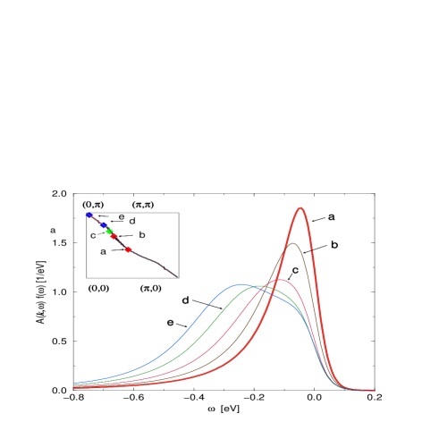
Figure 20: Product of spectral density and Fermi distribution function at different points of the Fermi surface, shown at the insert. Spin - fermion model, correlation length $\xi=3a$ Sch .

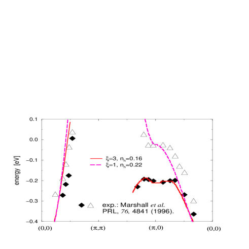
Figure 21: Position of the maximum of spectral density for two values of correlation length $\xi$ and hole concentration, calculated for spin - fermion model Sch in comparison with ARPES data of Ref.Marsh for $Bi_{2}Sr_{2}Ca_{1-x}Dy_{x}Cu_{2}O_{8+\delta}$ with $x=1$ (triangles) and $x=0.175$ (diamonds).

In Fig.21 from Sch we show calculated (for spin - fermion model with interaction (6), static limit) positions of the maximum of $A(\omega{\bf k})$ for two different concentrations of holes and appropriate experimental ARPES - data of Ref.Marsh for $Bi_{2}Sr_{2}Ca_{1-x}Dy_{x}Cu_{2}O_{8+\delta}$. These maxima positions in $(\omega,{\bf k})$ plane, obtained from ARPES, in fact determine (for Fermi - liquid like system) the experimental dispersion curves of quasiparticles (Cf. Fig.18(a)). For overdoped system the values of $n_{h}=0.22$ and $\xi=a$ were assumed. The results show rather well defined branches of the spectrum both in the direction of diagonal of the Brillouin zone, as well as in the $(0,0)-(\pi,0)$ direction. For underdoped system the values of $n_{h}=0.16$ and $\xi=3a$ were used. In this case, in diagonal direction we can again see the crossing of the spectrum with the Fermi level, while close to the “hot spots” in the vicinity of $(\pi,0)$ the smeared maximum of the spectral density remains approximately $200meV$ lower than the Fermi level (pseudogap behavior). In general, the agreement of theoretical model and experiment is rather encouraging.

Consider now the single - electron density of states:

$$N(E)=\sum_{\bf p}A(E,{\bf p})=-\frac{1}{\pi}\sum_{\bf p}ImG^{R}(E{\bf p})$$ (25)

defined by the integral of spectral density $A(E{\bf p})$ over Brillouin zone. Detailed calculations of the density of states in the “hot spots” model were performed in Ref.KS . For typical value of $t^{\prime}/t=-0.4$ rather smooth suppression of the density of states (pseudogap) was obtained. This drop in the density of states is relatively weakly dependent on the value of correlation length $\xi$. At the same time, for $t^{\prime}/t=-0.6$ (non characteristic for HTSC – cuprates) the “hot spots” on the Fermi surface still exist, but pseudogap in the density of states is practically invisible. Only the strong smearing of Van - Hove singularity, existing for the system without fluctuations, is clearly observed.

In “hot patches” model the use of (20) and (21) leads to the spectral density on these patches qualitatively similar to that shown in Fig.19 C91a ; McK . On “cold”parts of the Fermi surface the spectral density reduces to $\delta$-function, typical for Fermi - liquid (gas) (Cf. Fig.18 (a)). The density of states can be written as:

$$N(E)=-\frac{1}{\pi}N_{0}(0)\int_{0}^{2\pi}\frac{d\phi}{2\pi}\int\limits_{-\infty}^{\infty}d{\xi_{p}}ImG^{R}(E\xi_{p})=\frac{4\alpha}{\pi}N_{W}(E)+(1-\frac{4\alpha}{\pi})N_{0}(0)$$ (26)

where $N_{0}(0)$ - is the density of states of free electrons at the Fermi level, while $N_{W}(E)$ - is the density of states of one - dimensional model (square Fermi surface), obtained previously in Refs.C1 ; C2 ; C79 .

Let us quote some more detailed results for (artificial enough) limit of very large correlation lengths $\xi\to\infty$ (“toy” – model). In this case the whole perturbation series for the electron scattered by fluctuations is easily summed C1 ; C2 and an exact analytic solution for the Green’ function is obtained in the following form PS :

$$G(\epsilon_{n},p)=\int\limits_{0}^{\infty}dD{\cal P}(D)\frac{i\epsilon_{n}+\xi_{p}}{(i\epsilon_{n})^{2}-\xi_{p}^{2}-D(\phi)^{2}},$$ (27)

where $D(\phi)$ is defined for $0\leq\phi\leq\frac{\pi}{2}$ as:

$$D(\phi)=\left\{\begin{array}[]{ll}D&,0\leq\phi\leq\alpha,\>\frac{\pi}{2}-\alpha\leq\phi\leq\frac{\pi}{2}\\ 0&,\alpha\leq\phi\leq\frac{\pi}{2}-\alpha\end{array}\right.$$ (28)

For other values of $\phi$ the value of $D(\phi)$ is determined by obvious symmetry analogously to (28).

The amplitude of dielectric gap $D$ is random and distributed according to Rayleigh distribution C79 (its phase is also random and distributed homogeneously on the interval $(0,2\pi)$):

$${\cal P}(D)=\frac{2D}{W^{2}}exp\left(-\frac{D^{2}}{W^{2}}\right)$$ (29)

Thus, on the “hot patches” the Green’s function has the form of “normal” Gorkov’s function, averaged over spatially homogeneous fluctuations of dielectric gap $D$, distributed according to 29. “Anomalous” Gorkov’s function is, however, zero due to random phases of dielectric gap $D$, which corresponds to the absence of the long - range order.

For finite correlation lengths $\xi$ the amplitude of our one - dimensional random “periodic” field is approximately constant on the lengths of the order of $\xi$, while its values in different regions with sizes of the order of $\sim\xi$ are random. The crossover from one region with approximately periodic field to the other also takes place at lengths of the order of $\xi$. The electron is effectively scattered only during this transition from one region to another, which takes a time of the order of $\sim\xi/v_{F}$, leading to effective damping of the order of $\sim v_{F}/\xi$. Interesting data on numerical modeling of our random field, for one - dimensional case, can be found in Ref.Tchern .

Outside “hot patches” (the second inequality in (28)) the Green’s function (27) just coincides with that of free electrons.

Density of states, corresponding to (27), has the form (26), where

$$\frac{N_{W}(E)}{N_{0}(0)}=\left|\frac{E}{W}\right|\int\limits_{0}^{\frac{E^{2}}{W^{2}}}d{\zeta}\frac{e^{-\zeta}}{\sqrt{\frac{E^{2}}{W^{2}}-\zeta}}=2\left|\frac{E}{W}\right|exp(-\frac{E^{2}}{W^{2}})Erfi(\frac{E}{W})$$ (30)

where $Erfi(x)$ – is the probability integral of imaginary argument.

Figure 22: Density of states for “hot patches” of different sizes PS : (1) – $\alpha=\pi/4$; (2) – $\alpha=\pi/6$; (3) – $\alpha=\pi/8$; (4) – $\alpha=\pi/12$; (5) – $\alpha=\pi/24$.

In Fig.22 we show density of states of our model for different values of parameter $\alpha$, i.e. for “hot patches” of different sizes. It is seen that the pseudogap in the density of states is rather fast smeared (or filled in) as “hot patches” become smaller. In some sense the effect of diminishing $\alpha$ is analogous to the effect of diminishing correlation length $\xi$ C79 , so that the approximation of $\xi\rightarrow\infty$, is probably not so very strong limitation of this model. Finite values of $\xi$ can be easily accounted using (20) and (21), leading to additional smearing of the pseudogap for smaller $\xi$. Note the general qualitative agreement of the form of the pseudogap in this model with those observed in tunneling experiments, e.g. shown in Figs.4,5.

III.4 Two-Particle Green’ Function and Optical Conductivity.

Remarkably, for these models it is possible to calculate explicitly also two - particle Green’s functions for the electron in the random field of short - range order fluctuations C91 ; C91a (Cf. also Ref. Sch ), taking into account all Feynman diagrams of perturbation series. As calculations for “hot spots” model require rather large numerical work due to the use of “realistic” spectrum of current carriers (3), we shall limit ourselves to the simplified analysis within “hot patches” model C99 .

On “cold” parts of the Fermi surface we shall assume the existence of some small static scattering of an arbitrary nature, describing it by phenomenological scattering frequency $\gamma$, assuming, in most cases, that $\gamma\ll W$, so that we may neglect this scattering on “hot patches”. Accordingly, on “cold” parts the electronic spectrum will be described by by usual expressions for the Green’s functions for the system with weak (static) scattering.

Consider first the limit of $\xi\rightarrow\infty$ , when the single - electron Green’s function has the form (27) and two - particle Green’s function can also be found exactly using methods of Refs.C1 ; C2 .

Conductivity in this model always consists of additive contributions from “hot” and “cold” parts of the Fermi surface, analogously to (26). In particular, for its real part in the limit of $\xi\to\infty$ we have:

$$Re\sigma(\omega)=\frac{4\alpha}{\pi}Re\sigma_{W}(\omega)+(1-\frac{4\alpha}{\pi})Re\sigma_{D}(\omega)$$ (31)

where, with the account of the results of Refs.C1 ; C2 :

$$Re\sigma_{W}(\omega)=\frac{\omega_{p}^{2}}{4}\frac{W}{\omega^{2}}\int\limits_{0}^{\omega^{2}/4W^{2}}d{\zeta}exp(-\zeta)\frac{\zeta}{\sqrt{\omega^{2}/4W^{2}-\zeta}}$$ (32)

where $\omega_{p}$ – is plasma frequency and

$$Re\sigma_{D}(\omega)=\frac{\omega_{p}^{2}}{4\pi}\frac{\gamma}{\omega^{2}+\gamma^{2}}$$ (33)

– the usual Drude - like contribution of “cold” parts.

Even in this simplest approximation the dependence of $Re\sigma$ on $\omega$ is quite similar to observed in the experiments PBT ; STP ; B1 ; B2 . It is characterized by narrow “Drude” peak at small frequencies and smooth pseudogap absorption maximum at $\omega\sim 2W$. As scattering frequency $\gamma$ on “cold” parts grows, characteristic “Drude” peak at small frequencies is suppressed.

More realistic case of finite correlation lengths of fluctuations of “antiferromagnetic” short range order $\xi$ in (11) can be analyzed using (20), (21). Vertex part $J^{RA}(\epsilon,\xi_{\bf p};\epsilon+\omega,\xi_{\bf p+q})$, defining density - density response function (two - particle Green’ function) on “hot patches”an be determined from the following recursion procedure (details can be found in Refs.C91 ; C91a and also in Sch ), which takes into account all diagrams of perturbation series for interaction with fluctuations:

$$J^{RA}_{k-1}(\epsilon,\xi_{\bf p};\epsilon+\omega,\xi_{\bf p+q})=$$ (34)

$$=e+W^{2}v(k)G^{A}_{k}(\epsilon,\xi_{\bf p})G^{R}_{k}(\epsilon+\omega,\xi_{\bf p+q})J^{RA}_{k}(\epsilon,\xi_{\bf p};\epsilon+\omega,\xi_{\bf p+q})\times$$

$$\times\Biggl{\{}1+\frac{2iv_{F}\kappa k}{\omega-(-1)^{k}v_{F}q+v(k+1)W^{2}[G^{A}_{k+1}(\epsilon,\xi_{\bf p})-G^{R}_{k+1}(\epsilon+\omega,\xi_{\bf p+q})]}\Biggr{\}}$$

where $e$ – is electron charge, $R(A)$ denotes retarded (advanced) Green’s function, and the vertex part of interest to us is defined as $k=0$ term of this recursion procedure. Contribution of “hot patches” to conductivity $Re\sigma_{W}(\omega)$ in (31) is calculated as in Refs.C91 ; C91a , while $Re\sigma_{D}(\omega)$ is again determined by (33).

Typical results of such calculations are shown in Fig.23 for the case of incommensurate fluctuations.

Figure 23: Real part of conductivity as a function of frequency of external field, for different values of $\gamma$ and fixed correlation length $v_{F}\kappa=0.5W$. Conductivity is in units of $\omega_{p}^{2}/4\pi W$. (1)–$\gamma/W=0.2$; (2)–$\gamma/W=0.5$; (3)–$\gamma/W=1.0$. The size of “hot patches” $\alpha=\pi/6$. C99 . At the insert – calculated dependence of generalized scattering frequency $1/\tau$ (in units of $W$), as a function of frequency for different values of correlation length and fixed $\gamma=0.2W$. (1)–$v_{F}\kappa=0.1$; (2)–$v_{F}\kappa=0.5$; (3)–$v_{F}\kappa=1.0$ Str

The use of combinatorics of spin - fermion model leads to rather insignificant quantitative changes. The general qualitative picture remains the same also for commensurate case C99 . Conductivity is always characterized by narrow enough “Drude” peak in the region of small frequencies $\omega<\gamma$, originating from “cold” parts of the Fermi surface and a smooth maximum in the region of $\omega\sim 2W$, corresponding to the absorption through the pseudogap opened at the “hot patches’.’ “Drude” peak is rapidly suppressed as $\gamma$ grows. Dependence on correlation length of fluctuations $\xi=\kappa^{-1}$ in most interesting parameter region is weak enough. This qualitative picture is very similar to experimental dependencies observed for many HTSC – systems PBT ; STP ; B1 ; B2 , typical data were shown above in Fig.9. In this model we can also calculate the imaginary part of conductivity and the parameters of the generalized Drude model (1), (2) Str . Calculated $1/\tau(\omega)$ is shown at the insert in Fig.23 and demonstrates pseudogap behavior in the frequency region of $\omega<W$, quite analogous to that shown in Fig.10. Apparently it is not difficult to fit experimental data to our dependences using the known values of $\omega_{p}\sim 1.5-2.5eV$ and $2W\sim 0.1eV$, as well as “experimental ” values of $\gamma$, determined from the width of “Drude” peak, and varying “free” parameters $\alpha$ (the size of “hot patches”) and $\xi$ (the value of this can also be taken from other experiments Sch ).

IV Superconductivity in the Pseudogap State.

IV.1 Gorkov’s Equations.

At present there is no agreement on microscopic mechanism of Cooper pairing in HTSC - cuprates. The only well established fact is the anisotropic nature of pairing with $d$-wave symmetry Legg ; TsuK , though even here some alternative points of view exist. Apparently, the majority of researchers are inclined to believe in some kind pairing mechanism due to an exchange by spin (antiferromagnetic) excitations. A recent review of these theories can be found in Ref. Iz . Typical example of such a theory is the model of “nearly antiferromagnetic” Fermi - liquid (spin - fermion model), intensively developed by Pines and his collaborators Mont1 ; Mont2 . This model assumes that electrons interact with spin fluctuations and the form of this interaction (6) is restored, as mentioned above, from the fit to NMR experiments. MilMon . This approach continues to develop rapidly, we can only mention the very recent papers AC ; ACS ; ACF . There exist rather convincing experimental facts supporting this mechanism of pairing Iz ; ACSc . At the same time interaction of the form of (6) can be also responsible, as we shown above, for the formation of “dielectric” pseudogap already at high enough temperatures. Unfortunately, up to now there are no papers analyzing both the pseudogap formation and superconductivity within the single approach of spin - fermion model.

On the other hand rephrasing the quotation from Landau on Coulomb interaction, cited in Maks , we can only say that electron - phonon interaction was also “not canceled by anybody”, as a matter of fact as a possible mechanism of pairing in cuprates also. The review of appropriate calculations with rather impressive results can be found in Maks ; MKul and in earlier Ref.VLMaks . Probably the main difficulty for the models based on electron - phonon interaction in cuprates remains the established $d$-wave symmetry of Cooper pairs. However, there exist interesting attempts to explain the anisotropic pairing within the electron - phonon mechanism Maks ; MKul , as well as serious doubts in the effectiveness of spin - fluctuation mechanism Maks .

The author of the present review is not inclined to join either of these positions, being convinced that these (or similar FrK ) more or less “traditional” mechanisms are apparently decisive for the microscopics of HTSC. Anyhow, in the following we shall not even discuss some other more “radical” approaches, e.g. those developed in different variants and for many years models, based on the concept of Luttinger liquid PWA , mainly because of the absence there of any “stable” results and conclusions.

Significant renormalization of electronic spectrum due to the pseudogap formation inevitably leads to a strong change of properties of the system in superconducting state. In the scenario of pseudogap formation due to fluctuations of “dielectric” short - range order (AFM, SDW or CDW) we can speak precisely about the influence of the pseudogap upon superconductivity. In this formulation the analysis can be done even without assuming specific pairing mechanism, as it is done e.g. in the problem of the influence of structural disordering, impurities etc. From the physical point of view the least justified is the used above assumption of static nature of short - range order fluctuations, as dynamics of these fluctuations (e.g. in the model based on (6)) is apparently decisive at low enough temperatures (in superconducting phase), being responsible also for the pairing mechanism itself. We deliberately use these simplification as the full self - consistent solution of the problem within the model with dynamics seems to be out of reach, at least at present. Besides, in the following we shall only use the most simplified “hot patches” model . For generality we analyze both $s$-wave and $d$-wave pairing.

So, in the spirit of the previous discussion we shall not concentrate on any concrete microscopic mechanism of pairing and just assume the simplest possible BCS - like model, where the pairing is due to some kind attractive “potential” of the following form:

$$V_{sc}({\bf p,p^{\prime}})=V(\phi,\phi^{\prime})=-Ve(\phi)e(\phi^{\prime}),$$ (35)

where $\phi$ – is polar angle defining the direction of electron momentum ${\bf p}$ in highly - conducting plane, while for $e(\phi)$ we shall use the simple model dependence:

$$e(\phi)=\left\{\begin{array}[]{ll}1&(\mbox{ $s$-wave pairing})\\ \sqrt{2}\cos(2\phi)&(\mbox{ $d$-wave pairing})\end{array}.\right.$$ (36)

Attractive interaction constant $V$ is assumed, as usual, to be nonzero in some energy interval of the width $2\omega_{c}$ around the Fermi level ($\omega_{c}$ – is some characteristic frequency of excitations, responsible for attraction of electrons). The model interaction of the type of (35) was successfully used e.g. in Refs.Bork ; Fehr for the analysis of impurities influence on anisotropic Cooper pairing.

Superconducting energy gap in this case takes the following form:

$$\Delta({\bf p})\equiv\Delta(\phi)=\Delta e(\phi).$$ (37)

In the following, just not to make expressions too long, we shall use the notation of $\Delta$ instead of $\Delta(\phi)$, writing the angular dependence explicitly only when it will be necessary.

In superconducting state the perturbation theory for electron interaction with AFM fluctuations (11) should be built on “free” normal and anomalous Green’s functions of a superconductor:

$$G_{00}(\varepsilon_{n}{\bf p})=-\frac{i\varepsilon_{n}+\xi_{\bf p}}{\varepsilon_{n}^{2}+\xi^{2}_{\bf p}+|\Delta|^{2}};\quad F^{+}_{00}(\varepsilon_{n}{\bf p})=\frac{\Delta^{*}}{\varepsilon_{n}^{2}+\xi^{2}_{\bf p}+|\Delta|^{2}}$$ (38)

In this case we can formulate the direct analog of approximation (19) also in superconducting phase KS2000 . The contribution of an arbitrary diagram of the $N$-th order in interaction (10) to either normal or anomalous Green’ function consists of a product of $N+1$ “free” normal $G_{0k_{j}}$ or anomalous $F^{+}_{0k_{j}}$ Green’ functions with renormalized (in a certain way) frequencies and gaps. Here $k_{j}$ – is the number of interaction lines surrounding the $j$-th (from the beginning of the diagram) electronic line. As in normal phase the contribution of an arbitrary diagram is defined by some set of integers $k_{j}$, and each diagram with intersecting interaction lines becomes equal to some diagram without intersections. For this last reason we can analyze only diagrams with no intersections of interaction lines, taking all the other diagrams into account by the same combinatorial factors $v(k)$, attributed to interaction lines as in the normal phase. As a result we obtain an analog of Gorkov’s equations AGD . Accordingly there appears now a system of two recursion equations for normal and anomalous Green’s functions:

$$G_{k}=G_{0k}+G_{0k}\tilde{G}G_{k}-G_{0k}\tilde{F}F^{+}_{k}-F_{0k}\tilde{G}^{*}F^{+}_{k}-F_{0k}\tilde{F}^{+}G_{k}$$

$$F^{+}_{k}=F^{+}_{0k}+F^{+}_{0k}\tilde{G}G_{k}-F^{+}_{0k}\tilde{F}F^{+}_{k}+G^{*}_{0k}\tilde{G}^{*}F^{+}_{k}+G^{*}_{0k}\tilde{F}^{+}G_{k}$$ (39)

where

$$\tilde{G}=W^{2}v(k+1)G_{k+1};\quad\tilde{F}^{+}=W^{2}v(k+1)F^{+}_{k+1}$$ (40)

$$G_{0k}(\varepsilon_{n}{\bf p})=-\frac{i\varepsilon_{n}+(-1)^{k}\xi_{\bf p}}{\tilde{\varepsilon}_{n}^{2}+\xi^{2}_{\bf p}+|\tilde{\Delta}|^{2}};\quad F^{+}_{0k}(\varepsilon_{n}{\bf p})=\frac{\tilde{\Delta}^{*}}{\tilde{\varepsilon}_{n}^{2}+\xi^{2}_{\bf p}+|\tilde{\Delta}|^{2}}$$ (41)

and we introduced the abovementioned renormalized frequency $\tilde{\varepsilon}$ and gap $\tilde{\Delta}$:

$$\tilde{\varepsilon}_{n}=\eta_{k}\varepsilon_{n};\quad\tilde{\Delta}=\eta_{k}\Delta;\quad\eta_{k}=1+\frac{kv_{F}\kappa}{\sqrt{\varepsilon_{n}^{2}+|\Delta|^{2}}}$$ (42)

similar to those appearing in the analysis of a superconductor with impurities AGD .

Both normal and anomalous Green’s functions of a superconductor with pseudogap are defined from (39) at $k=0$ and represent the complete sum of all diagrams of perturbation series over interaction of superconducting electron with fluctuations of AFM short - range order.

In fact we just consider Gorkov’s Green’s functions averaged over an ensemble of random (Gaussian) fluctuations of short - range order, in many respect analogously to the similar analysis of the case of impure superconductors AGD . Here we assume here the self - averaging property of superconducting order parameter (energy gap) $\Delta$, which allows to average it independently of electronic Green’s functions in diagrammatic series. Usual arguments for the possibility of such independent averaging are the following Gor ; Genn ; Scloc : the value of $\Delta$ changes on characteristic length scale of the order of coherence length $\xi_{0}\sim v_{F}/\Delta$ of BCS theory, while Green’s functions oscillate on much shorter length scale of the order of interatomic distance. Naturally, this last assumption becomes wrong if a new characteristic length $\xi\to\infty$ appears in electronic subsystem. At the same time, until this AFM correlation length $\xi\ll\xi_{0}$ (i.e. when AFM fluctuations correlate on lengths smaller than characteristic size of Cooper pairs), the assumption of self - averaging nature of $\Delta$ is apparently still conserved, being broken only in the region of $\xi>\xi_{0}$. As a result we can use the standard approach of the theory of disordered superconductors (mean - field approximation in terms of Ref.KSad ). Possible role of non - self - averaging $\Delta$ KSad will be analyzed later. Note that in real HTSC - cuprates apparently always we have $\xi\sim\xi_{0}$, so that they belong to the region of parameters most difficult for theory.

IV.2 Critical Temperature and the Temperature Dependence of the Gap.

Energy gap of a superconductor is defined by the equation:

$$\Delta({\bf p})=-T\sum_{\bf p^{\prime}}\sum_{\varepsilon_{n}}V_{sc}({\bf p,p^{\prime}})F(\varepsilon_{n}{\bf p^{\prime}})$$ (43)

On flat parts of the Fermi surface the anomalous Green’s function is determined by recursion procedure (39). On the rest (“cold”) part of the Fermi surface scattering by AFM fluctuations is absent (in our model) and the anomalous Green’s function has the form as in Eq.(38). The results of numerical calculations of the temperature dependence of the gap for different values of correlation length of short - range order fluctuations $\xi$ can be found in Ref.KS2000 . These dependences are more or less of the usual form.

Equation for the critical temperature of superconducting transition $T_{c}$ follows immediately from (43) as $\Delta\to 0$. Calculated in Ref.KS2000 dependences of $T_{c}$ on the width of the pseudogap $W$ and correlation length (parameter $\kappa=\xi^{-1}$) are shown in Fig.24, where $T_{c0}$ – is transition temperature in the absence of the pseudogap. In this calculations we have, rather arbitrarily, taken the value of $\alpha=\pi/6$, which is pretty close to the experimental data of Ref.Onell .

Figure 24: Dependence of superconducting critical temperature on the width of the pseudogap $W$ and correlation length of AFM fluctuations (parameter $\kappa=\xi^{-1}$): $\frac{v_{F}\kappa}{W}=0.1$ (1);  $\frac{v_{F}\kappa}{W}=1.0$ (2);  $\frac{v_{F}\kappa}{W}=10.0$ (3). Dashed line — $\kappa=0$ PS . At the insert: dependence of $T_{c}$ on $\kappa$ for $\frac{W}{T_{c0}}=5$ KS2000 .

The general qualitative conclusion is that pseudogap suppresses superconductivity due to partial “dielectrization” of electronic spectrum on “hot patches” of the Fermi surface. This suppression is maximal for $\kappa=0$ (infinite correlation length of AFM fluctuations) PS ; KSad and diminishes with diminishing values of correlation length, which qualitatively corresponds to the observed phase diagram of HTSC - systems. As noted above, parameters of our model are to be considered as phenomenological. E.g. the effective width of the pseudogap $2W$ may be, apparently, identified as $E_{g}$, the experimental values of which and dependence on doping are shown in Fig.8 for $YBCO$. Experimental data on the values of correlation length $\xi$ and its temperature dependence are rather incomplete. Indirectly this information may be extracted from NMR experiments MilMon ; Sch . Direct neutron scattering data are not conclusive enough. As an example we shall mention the paper Bour , where the authors present some compilation of data on effective width of neutron scattering peak at the vector $(\pi/a,\pi/a)$ in $YBCO$ with different oxygen content. The inverse width of this peak can be naturally identified with the value of $\xi$. The authors of Ref.Bour observed an interesting correlation of superconducting critical temperature and thus defined values of $\xi^{-1}$, which is shown in Fig.25. Obviously, this dependence is in direct qualitative correspondence with dependence of $T_{c}$ on $\kappa=\xi^{-1}$, shown in Fig.24. Quantitative fit of these data to calculated dependences, following from our model, is apparently possible, but we must be also aware of rather incomplete information on doping dependence of parameter $W$.

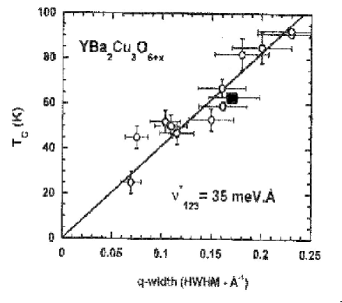
Figure 25: Temperature of superconducting transition $T_{c}$ as a function of the width of neutron scattering peak at ${\bf q}=(\pi/a,\pi/a)$, which is identified with the inverse of correlation - length of short - range order fluctuations Bour .

In particular, it is not clear, whether there is any deep physical meaning of $E_{g}\sim W$ going to zero at some “critical” doping as shown in fig.8. Pseudogap influence on electronic properties may disappear also due to correlation length $\xi$ becoming just smaller, which leads not to the “closing”, but to the “filling” of the pseudogap in the density of states. However, if we accept the data of Fig.8 on the width of the pseudogap TL , then our parameter $2W$ drops from the values of the order of $700K$ at hole concentration $p=0.05$ to the values of the order of $T_{c}\sim 100K$ near optimal doping $p=0.17$, going to zero at $p=0.19$. If we assume the validity of microscopic expression (9) for $W$, following from the theory of “nearly antiferromagnetic” Fermi - liquid, this concentration dependence may be attributed to the appropriate dependence of local spin $<{\bf S}_{i}^{2}>$ on $Cu$ - ion. The author is unaware of any direct data of this sort, but we may note Ref.JTal , where the disappearance of effective interaction with antiferromagnetic fluctuations at $p=0.19$ was demonstrated from some fit to experimental data on NMR relaxation.

Let us stress once again, that the above theoretical results are valid only assuming self - averaging nature of superconducting order parameter (gap) as averaged over AFM fluctuations (random mean - field approximation KSad ), which is apparently true for not very large values of correlation length $\xi<\xi_{0}$, where $\xi_{0}$ – is the coherence length of a superconductor (the size of Cooper pairs at $T=0$). For $\xi\gg\xi_{0}$, as we shall see below, important effects due the absence of self - averaging appear, leading to characteristic “tails” in the temperature dependence of the average gap in the region of $T_{c}<T<T_{co}$ KSad .

IV.3 Cooper Instability.

It is well known that the critical temperature may be determined also in another way, that is from the equation for Cooper instability of the normal phase:

$$1-V\chi(0,0)=0$$ (44)

where $\chi(0,0)$ is the generalized Cooper susceptibility:

$$\chi({\bf q}0;T)=-T\sum_{\varepsilon_{n}}\sum_{\bf p}G(\varepsilon_{n}{\bf p+q})G(-\varepsilon_{n}{\bf p})e^{2}(\phi)\Gamma(\varepsilon_{n},-\varepsilon_{n},\bf q)$$ (45)

Here we have to calculate the “triangular” vertex part $\Gamma(\varepsilon_{n},-\varepsilon_{n},\bf q)$, describing electron interaction with AFM fluctuations. For one - dimensional analogue of our problem (and for real frequencies, $T=0$) appropriate recursion procedure was formulated in Refs.C91 . For our two - dimensional model this procedure was used in calculations of optical conductivity, as discussed above C99 . This procedure is easily generalized for the case of Matsubara frequencies KS2000 . Below, for definiteness, we assume $\varepsilon_{n}>0$. Then, similarly to (34), we have:

$$\Gamma_{k-1}(\varepsilon_{n},-\varepsilon_{n},{\bf q})=1+$$

$$+W^{2}v(k)G_{k}\bar{G}_{k}\Biggl{\{}1+\frac{2ikv_{F}\kappa}{2i\varepsilon_{n}-(-1)^{k}v_{F}q-W^{2}v(k+1)(G_{k+1}-\bar{G}_{k+1})}\Biggr{\}}\Gamma_{k}(\varepsilon_{n},-\varepsilon_{n},{\bf q})$$

$$\Gamma(\varepsilon_{n},-\varepsilon_{n},{\bf q})\equiv\Gamma_{0}(\varepsilon_{n},-\varepsilon_{n},{\bf q})$$ (46)

where $G_{k}=G_{k}(\varepsilon_{n}{\bf p+q})$ and $\bar{G}_{k}=G_{k}(-\varepsilon_{n},{\bf p})$ are calculated according to (21).

To calculate $T_{c}$ we need the vertex at ${\bf q}=0$. Then $\bar{G}_{k}=G^{*}_{k}$ and vertices $\Gamma_{k}$ become real, which leads to considerable simplification of the procedure (46).

The following exact relation holds, similar to Ward identity KS2000 :

$$G(\varepsilon_{n}{\bf p})G(-\varepsilon_{n}{\bf p})\Gamma(\varepsilon_{n},-\varepsilon_{n},0)=-\frac{ImG(\varepsilon_{n}{\bf p})}{\varepsilon_{n}}$$ (47)

Numerical calculations fully confirm this relation, demonstrating the self - consistency of our recurrence relations for single - particle Green’s function and vertex part. The relation (47) leads to the equivalence of $T_{c}$ equation, derived from Cooper instability, and $T_{c}$ equation, obtained from the linearized gap equation, though the recurrence procedures used to derive both equations (accounting for AFM fluctuations) seem to be quite different.

IV.4 Ginzburg-Landau Equations and Basic Properties of a Superconductor with the Pseudogap close to $T_{c}$.

Ginzburg - Landau expansion for the difference of free - energy density of superconducting and normal state can be written in standard form:

$$F_{s}-F_{n}=A|\Delta_{\bf q}|^{2}+q^{2}C|\Delta_{\bf q}|^{2}+\frac{B}{2}|\Delta_{\bf q}|^{4},$$ (48)

where $\Delta_{\bf q}$ – is the amplitude of Fourier - component of superconducting order parameter:

$$\Delta(\phi,{\bf q})=\Delta_{\bf q}e(\phi).$$ (49)

This expansion (48) is determined by loop - expansion diagrams for the free - energy of an electron in the field of random fluctuations of order - parameter with small wave - vector ${\bf q}$ PS .

Let us write the coefficients of Ginzburg - Landau expansion in the following form:

$$A=A_{0}K_{A};\qquad C=C_{0}K_{C};\qquad B=B_{0}K_{B},$$ (50)

where $A_{0}$, $C_{0}$ and $B_{0}$ are standard expressions for these coefficients for the case of isotropic $s$-wave pairing:

$$A_{0}=N_{0}(0)\frac{T-T_{c}}{T_{c}};\qquad C_{0}=N_{0}(0)\frac{7\zeta(3)}{32\pi^{2}}\frac{v_{F}^{2}}{T_{c}^{2}};\qquad B_{0}=N_{0}(0)\frac{7\zeta(3)}{8\pi^{2}T_{c}^{2}},$$ (51)

The all changes of these coefficients due to the appearance of the pseudogap are contained in dimensionless coefficients $K_{A}$, $K_{C}$ and $K_{B}$. In the absence of the pseudogap all these coefficients are equal to 1, except $K_{B}=3/2$ in case of $d$-wave pairing.

Consider again the generalized Cooper susceptibility (45). Then the coefficients $K_{A}$ and $K_{C}$ can be written as KS2000 :

$$K_{A}=\frac{\chi(00;T)-\chi(00;T_{c})}{A_{0}}$$ (52)

$$K_{C}=\lim_{q\to 0}\frac{\chi({\bf q}0;T_{c})-\chi(00;T_{c})}{q^{2}C_{0}}$$ (53)

Then all calculations can be made using the recurrence procedure (46).

To find the coefficient $B$, in general case, we need more complicated procedure. Significant simplifications appear if we limit ourselves, for terms of the order of $|\Delta_{\bf q}|^{4}$ in free energy, by the usual case of $q=0$. Then the coefficient $B$ may be determined directly from the anomalous Green’s function $F$, i.e. from the recurrence procedure (39) KS2000 .

In the limit of $\xi\to\infty$ all coefficients of Ginzburg - Landau expansion may be obtained analytically PS , using the exact solution for the Green’s functions discussed above.

Ginzburg - Landau expansion defines two characteristic lengths of superconducting state: coherence length and penetration depth (of magnetic field). Coherence length at given temperature $\xi(T)$ determines the length scale of inhomogeneities of the order parameter $\Delta$:

$$\xi^{2}(T)=-\frac{C}{A}.$$ (54)

In the absence of the pseudogap:

$$\xi_{BCS}^{2}(T)=-\frac{C_{0}}{A_{0}},$$ (55)

$$\xi_{BCS}(T)\approx 0.74\frac{\xi_{0}}{\sqrt{1-T/T_{c}}},$$ (56)

where $\xi_{0}=0.18v_{F}/T_{c}$. In our model:

$$\frac{\xi^{2}(T)}{\xi_{BCS}^{2}(T)}=\frac{K_{C}}{K_{A}}.$$ (57)

Appropriate dependences of $\xi^{2}(T)/\xi_{BCS}^{2}(T)$ on the width of the pseudogap $W$ and correlation length of fluctuations (parameter $\kappa$) , for the case of $d$-wave pairing were calculated in Ref.KS2000 and found to be smooth, with relatively insignificant changes of the ratio (57) itself.

For the penetration depth of a superconductor without the pseudogap we have:

$$\lambda_{BCS}(T)=\frac{1}{\sqrt{2}}\frac{\lambda_{0}}{\sqrt{1-T/T_{c}}},$$ (58)

where $\lambda_{0}^{2}=\frac{mc^{2}}{4\pi ne^{2}}$ defines penetration depth at $T=0$. In general case:

$$\lambda^{2}(T)=-\frac{c^{2}}{32\pi e^{2}}\frac{B}{AC}.$$ (59)

Then for our model we have:

$$\frac{\lambda(T)}{\lambda_{BCS}(T)}=\left(\frac{K_{B}}{K_{A}K_{C}}\right)^{1/2}.$$ (60)

Dependences of this ratio on the pseudogap width and correlation length were also calculated for the case of $d$-wave pairing in Ref.KS2000 and found to be relatively small.

Close to $T_{c}$ the upper critical field $H_{c2}$ is determined via Ginzburg - Landau coefficients as:

$$H_{c2}=\frac{\phi_{0}}{2\pi\xi^{2}(T)}=-\frac{\phi_{0}}{2\pi}\frac{A}{C},$$ (61)

where $\phi_{0}=c\pi/e$ – is the magnetic flux quantum. Then the slope of the upper critical field near $T_{c}$ is given by:

$$\left|\frac{dH_{c2}}{dT}\right|_{T_{c}}=\frac{24\pi\phi_{0}}{7\zeta(3)v_{F}^{2}}T_{c}\frac{K_{A}}{K_{C}}.$$ (62)

Graphic dependences of this slope $\left|\frac{dH_{c2}}{dT}\right|_{T_{c}}$, at temperature $T_{c0}$ on the effective width of the pseudogap $W$ and correlation length parameter $\kappa$ can also be found in Ref.KS2000 . The slope of the upper critical field for the case of large enough correlation lengths drops fast with the growth of the pseudogap width. However, for short enough correlation lengths some growth of this slope can also be observed at small pseudogap widths. At fixed pseudogap width the slope of $H_{c2}$ grows significantly with the drop of correlation length of fluctuations.

Finally, consider the specific heat discontinuity (jump) at the transition point:

$$\frac{C_{s}-C_{n}}{\Omega}=\frac{T_{c}}{B}\left(\frac{A}{T-T_{c}}\right)^{2},$$ (63)

where $C_{s},\>C_{n}$ – are the specific heats in superconducting and normal states respectively, $\Omega$ – is the sample volume. At temperature $T=T_{c0}$ and in the absence of the pseudogap ($W=0$):

$$\left(\frac{C_{s}-C_{n}}{\Omega}\right)_{T_{c0}}=N(0)\frac{8\pi^{2}T_{c0}}{7\zeta(3)}.$$ (64)

Then the relative specific heat discontinuity in our model can be written as:

$$\frac{(C_{s}-C_{n})_{T_{c}}}{(C_{s}-C_{n})_{T_{c0}}}=\frac{T_{c}}{T_{c0}}\frac{K_{A}^{2}}{K_{B}}.$$ (65)

Appropriate dependences on effective width of the pseudogap $W$ and correlation length parameter $\kappa$ for the case of $d$-wave pairing are shown in Fig.26. It is seen that the specific heat discontinuity is rapidly suppressed with the growth of the pseudogap width and, inversely, it grows with for shorter correlation lengths of AFM fluctuations.

Figure 26: Dependence of specific heat discontinuity on pseudogap width $W$ and correlation length of AFM fluctuations (parameter $\kappa=\xi^{-1}$): $\frac{v_{F}\kappa}{W}=0.1$ (1); $\frac{v_{F}\kappa}{W}=1.0$ (2);  $\frac{v_{F}\kappa}{W}=10.0$ (3). Dashed line — $\kappa=0$ PS . At the insert: dependence of specific heat discontinuity on $\kappa$ for $\frac{W}{T_{c0}}=5$.

For superconductors with $s$-wave pairing all the dependences are quite similar to that found above, the only difference is the larger scale of $W$ leading to significant changes of all characteristics of superconducting state, corresponding to larger stability of isotropic superconductors to partial “dielectrization” of electronic spectrum due to to pseudogap formation on “hot patches” of the Fermi surface PS ; KSad .

All these results are in complete qualitative agreement with experimental data on specific heat discontinuity discussed above TL ; Loram ; Lor . As can be seen from Fig.2, specific heat discontinuity is rapidly suppressed as system moves to underdoped region, where the pseudogap width grows as is seen from the data shown in Fig. 8.

IV.5 Effects due to non-Self-Averaging Nature of the Order-Parameter.

The above analysis of superconductivity assumed the self - averaging property of superconducting order parameter $\Delta$. This assumption is apparently justified in case of correlation length of fluctuations of (AFM) short - range order $\xi$ being small in comparison with characteristic size of Cooper pairs $\xi_{0}$ (coherence length of BCS theory). The opposite limit of $\xi\gg\xi_{0}$ can be analyzed within the exactly solvable model of the pseudogap state with $\xi\to\infty$, which was described above for the case of “hot patches” model in (27), (29) KSad .

Consider first superconductivity in a system with fixed dielectric gap $D$ on “hot patches” of the Fermi surface. The problem of superconductivity in a system with partial dielectrization of electron energy spectrum on certain parts of the Fermi surface was considered previously in a number of papers (cf. e.g. Refs.Kopaev ; Ginz ), and in the form most useful for our case in a paper by Bilbro and McMillan Bilb . Below we shall use some of the results of this paper. Again we assume the simplest BCS - like model of pairing interaction (35), (36).

For the fixed value of dielectric gap $D$ on “hot patches” of the Fermi surface superconducting gap equation, defining $\Delta$ for the case of $s$-wave pairing, takes the following form:

$$1=\lambda\int_{0}^{\omega_{c}}d\xi\left\{\tilde{\alpha}\frac{th\frac{\sqrt{\xi^{2}+D^{2}+\Delta^{2}(D)}}{2T}}{\sqrt{\xi^{2}+D^{2}+\Delta^{2}(D)}}+(1-\tilde{\alpha})\frac{th\frac{\sqrt{\xi^{2}+\Delta^{2}(D)}}{2T}}{\sqrt{\xi^{2}+\Delta^{2}(D)}}\right\}$$ (66)

where $\lambda=VN_{0}(0)$ – is dimensionless coupling constant of pairing interaction, $\tilde{\alpha}=\frac{4\alpha}{\pi}$. The first term in the r.h.s. of Eq.(66) corresponds to the contribution of “hot” (dielectrized or “closed”) parts of the Fermi surface, where electronic spectrum is given by Bilb : $E_{p}=\sqrt{\xi^{2}_{p}+D^{2}+\Delta^{2}}$, while the second term gives the contribution of “cold” (metallic or “open”) parts, where the spectrum has the usual BCS form: $E_{p}=\sqrt{\xi^{2}_{p}+\Delta^{2}}$. Eq. (66) determines superconducting gap $\Delta(D)$ at fixed value of dielectric gap $D$, which is different from zero on “hot patches”.

In case of $d$-wave pairing the analogous equation has the form:

$$1=\lambda\frac{4}{\pi}\int_{0}^{\omega_{c}}d\xi\left\{\int_{0}^{\alpha}d{\phi}e^{2}(\phi)\frac{th\frac{\sqrt{\xi^{2}+D^{2}+\Delta^{2}(D)e^{2}(\phi)}}{2T}}{\sqrt{\xi^{2}+D^{2}+\Delta^{2}(D)e^{2}(\phi)}}+\int_{\alpha}^{\pi/4}d{\phi}e^{2}({\phi})\frac{th\frac{\sqrt{\xi^{2}+\Delta^{2}(D)e^{2}(\phi)}}{2T}}{\sqrt{\xi^{2}+\Delta^{2}(D)e^{2}(\phi)}}\right\}$$ (67)

From these equation it can be seen that $\Delta(D)$ diminishes with the growth of $D$, while $\Delta(0)$ coincides with the usual gap $\Delta_{0}$ in the absence of dielectrization on flat parts of the Fermi surface and appearing at temperature $T=T_{c0}$, defined by the equation:

$$1=\lambda\int_{0}^{\omega_{c}}d\xi\frac{th\frac{\xi}{2T_{c0}}}{\xi}$$ (68)

both for $s$-wave and $d$-wave pairing.

For $D\to\infty$ the first terms of Eqs.(66),(67) tend to zero, so that the appropriate equations for $\Delta_{\infty}=\Delta(D\to\infty)$ are:

$$1=\lambda\int_{0}^{\omega_{c}}d\xi(1-\tilde{\alpha})\frac{th\frac{\sqrt{\xi^{2}+\Delta^{2}_{\infty})}}{2T}}{\sqrt{\xi^{2}+\Delta^{2}_{\infty}}}\quad\mbox{($s$-wave pairing)}$$ (69)

$$1=\lambda\frac{4}{\pi}\int_{0}^{\omega_{c}}d\xi\int_{\alpha}^{\pi/4}d{\phi}e^{2}({\phi})\frac{th\frac{\sqrt{\xi^{2}+\Delta^{2}_{\infty}e^{2}(\phi)}}{2T}}{\sqrt{\xi^{2}+\Delta^{2}_{\infty}e^{2}(\phi)}}\quad\mbox{($d$-wave pairing)}$$ (70)

Equation (69) coincides with gap equation for the case of $D=0$ with “renormalized” coupling constant $\tilde{\lambda}=\lambda(1-\tilde{\alpha})$, so that for the case of $s$-wave pairing:

$$\Delta_{\infty}=\Delta_{0}(\tilde{\lambda}=\lambda(1-\tilde{\alpha}))$$ (71)

and non zero superconducting gap in the limit of $D\to\infty$ appears at $T<T_{c\infty}$

$$T_{c\infty}=T_{c0}(\tilde{\lambda}=\lambda(1-\tilde{\alpha})).$$ (72)

In the case of $d$-wave pairing from Eq.(70) we get:

$$T_{c\infty}=T_{c0}(\tilde{\lambda}=\lambda(1-\alpha_{d}))$$ (73)

where

$$\alpha_{d}=\tilde{\alpha}+\frac{\sin\pi\tilde{\alpha}}{\pi}$$ (74)

defines the “effective” size of flat parts of the Fermi surface for the case of $d$-wave pairing. Thus, for $T<T_{c\infty}$ superconducting gap is nonzero for any values of $D$ and drops form the value of $\Delta_{0}$ to $\Delta_{\infty}$ with the growth of $D$. For $T_{c\infty}<T<T_{c0}$ the gap is nonzero only for $D<D_{max}$. Appropriate dependences of $\Delta$ on $D$ can easily be obtained by numerical solution of Eqs. (66) and (67).

In our model of the pseudogap state dielectric gap $D$ is not fixed but random and distributed according to (29). The above results should be averaged over these fluctuations. It is important that within this model we can directly calculate and exactly calculate superconducting gap $\Delta$, averaged over the fluctuations of $D$:

$$<\Delta>=\int_{0}^{\infty}dD{\cal P}(D)\Delta(D)=\frac{2}{W^{2}}\int_{0}^{\infty}dDDe^{-\frac{D^{2}}{W^{2}}}\Delta(D)$$ (75)

The dependences of $\Delta(D)$ described above lead to the average gap (75) being formally nonzero up to the temperature $T=T_{c0}$, i.e. the temperature of superconducting transition in the absence of pseudogap anomalies. At the same time, the temperature of superconducting transition $T_{c}$ in a superconductor with the pseudogap is, obviously, smaller than $T_{c0}$ PS . This paradoxical behavior of $<\Delta>$ apparently can be explained by $D$-fluctuation induced appearance of local regions in the sample with $\Delta\neq 0$ (superconducting “drops”) in the whole temperature region of $T_{c}<T<T_{c0}$, with superconducting coherence appearing only for $T<T_{c}$. Of course, the full justification of this qualitative picture can be obtained only after the analysis of more realistic model with finite correlation length $\xi$ of AFM fluctuations . At the same time, simplicity of our “toy” model with $\xi\to\infty$ allows to get an exact solution for $<\Delta>$ immediately.

To determine superconducting transition temperature $T_{c}$ in a sample as a whole we may use the standard mean - field approximation procedure to average over random short - range order fluctuations (similar approach is used in the theory of impure superconductors Scloc ), which assumes the self - averaging of superconducting gap over fluctuations of $D$ (i.e., in fact, independence of $\Delta$ on fluctuations of $D$). Then the equations for this mean - field $\Delta_{mf}$ have the following form:

$$1=\lambda\int_{0}^{\omega_{c}}d\xi\left\{\tilde{\alpha}\frac{2}{W^{2}}\int_{0}^{\infty}dDDe^{-\frac{D^{2}}{W^{2}}}\frac{th\frac{\sqrt{\xi^{2}+D^{2}+\Delta^{2}_{mf}}}{2T}}{\sqrt{\xi^{2}+D^{2}+\Delta^{2}_{mf}}}+(1-\tilde{\alpha})\frac{th\frac{\sqrt{\xi^{2}+\Delta^{2}_{mf}}}{2T}}{\sqrt{\xi^{2}+\Delta^{2}_{mf}}}\right\}$$ (76)

for the case of $s$-wave pairing, and

$$1=\lambda\frac{4}{\pi}\int_{0}^{\omega_{c}}d\xi\left\{\frac{2}{W^{2}}\int_{0}^{\infty}dDDe^{-\frac{D^{2}}{W^{2}}}\int_{0}^{\alpha}d{\phi}e^{2}(\phi)\frac{th\frac{\sqrt{\xi^{2}+D^{2}+\Delta^{2}_{mf}e^{2}(\phi)}}{2T}}{\sqrt{\xi^{2}+D^{2}+\Delta^{2}_{mf}e^{2}(\phi)}}+\right.$$

$$\left.+\int_{\alpha}^{\pi/4}d{\phi}e^{2}({\phi})\frac{th\frac{\sqrt{\xi^{2}+\Delta^{2}_{mf}e^{2}(\phi)}}{2T}}{\sqrt{\xi^{2}+\Delta^{2}_{mf}e^{2}(\phi)}}\right\}$$ (77)

for the case of $d$-wave pairing. These equations are the limiting case (for $\xi\to\infty$) of superconducting gap equations analyzed above (43) using the recurrence procedure (39).

From (76) and (77) it is easy to get the appropriate $T_{c}$ - equations, giving the temperature at which the homogeneous gap $\Delta_{mf}$ first appears everywhere in the sample. For the case of $s$-wave pairing we have:

$$1=\lambda\left\{\tilde{\alpha}\frac{2}{W^{2}}\int_{0}^{\infty}dDDe^{-\frac{D^{2}}{W^{2}}}\int_{0}^{\omega_{c}}d\xi\frac{th\frac{\sqrt{\xi^{2}+D^{2}}}{2T_{c}}}{\sqrt{\xi^{2}+D^{2}}}+(1-\tilde{\alpha})\int_{0}^{\omega_{c}}d\xi\frac{th\frac{\xi}{2T_{c}}}{\xi}\right\}$$ (78)

In case of $d$-wave pairing we have just to replace $\tilde{\alpha}$ in (78) by “effective” $\alpha_{d}$ defined in (74). These equations for $T_{c}$ coincide with coincide with those obtained during the microscopic derivation of Ginzburg - Landau expansion in this model PS and with $\xi\to\infty$ limit of equations obtained using (39), (43). In general we always have $T_{c\infty}<T_{c}<T_{c0}$.

Temperature dependences of average gap $<\Delta>$ and mean - field gap $\Delta_{mf}$, obtained by numerical solution of our equations for the case of $s$-wave pairing, are shown in Fig.27 .

Figure 27: Temperature dependences of superconducting gaps $\Delta_{mf}$ (dots), $<\Delta>$ (full curves) and $\Delta_{0}$ (dashed curves) for the case of $s$-wave pairing KSad . 1. – $\lambda=0.4$; $\tilde{\alpha}=2/3$; $\omega_{c}/W=3$ ($T_{c}/T_{c0}=0.42$). 2. – $\lambda=0.4$; $\tilde{\alpha}=0.2$; $\omega_{c}/W=1$ ($T_{c}/T_{c0}=0.71$).

We see that $\Delta_{mf}$ goes to zero at $T=T_{c}<T_{c0}$, while $<\Delta>$ is nonzero up to $T=T_{c0}$ and characteristic “tails” in the temperature dependence of $<\Delta>$ in the region of $T_{c}<T<T_{c0}$, in our opinion, correspond to the abovementioned picture of superconducting “drops” appearing in this temperature interval, while superconductivity in a sample as a whole is absent. Note that temperature dependences of $<\Delta(T)>$ shown in Fig.27 are quite similar to those observed in underdoped cuprates via ARPES Nrm or specific heat measurements Lor , and shown in Figs. 3, 14, if we assume that $T_{c}$ observed in these samples corresponds to our mean - field $T_{c}$, while “drops” with $<\Delta>\neq 0$ exist in the region of $T>T_{c}$ up to $T_{c0}$, which is much higher than $T_{c}$. Non self - averaging nature of the gap in our model is also reflected in the fact that in the whole temperature region of $T<T_{c0}$ gap dispersion $<\Delta^{2}>-<\Delta>^{2}$ is different from zero, circumstantially confirming the proposed qualitative picture of “drops”. Of course, full justification of this picture is possible only with the account of finite values of $\xi$. Note that the value of $T_{c0}$ is not very well defined from the experimental point of view. Speaking above about superconducting transition temperature in the absence of the pseudogap we assumed the value of $T_{c0}$ of the order of $T_{c}$ observed for optimal doping. However, to compare the results shown in Fig.27 with data of Figs.3, 14 we need the values of $T_{c0}$ much higher than optimal $T_{c}$. in this sense the described picture of superconducting “drops” induced by “dielectric” gap fluctuations becomes not so very different from precursor pairing picture of superconducting pseudogap scenario. At the same time it is clear that the most part of data shown in Figs. 3, 14 may be explained by the existence of the pseudogap of dielectric nature, not by just discussed non self - averaging nature of superconducting $\Delta$. Note, for example, that superconducting gap obtained from tunneling data of Refs. Kras1 ; Kras2 (appearing on the “background” of much wider pseudogap) demonstrates “normal” temperature behavior going to zero at $T=T_{c}$.

Despite the fact that superconductivity in a sample as a whole for $T_{c}<T<T_{c0}$ is absent, the existence in this region of nonzero average $<\Delta>$ leads to anomalies in a number of observables, e.g. in tunneling density of states or spectral density measured via ARPES KSad .

In particular, the tunneling density of states for the case of $d$-wave pairing has the following form KSad :

$$\frac{N(E)}{N_{0}(0)}=\frac{4}{\pi}\frac{2}{W^{2}}\int_{0}^{\infty}dDDe^{-\frac{D^{2}}{W^{2}}}\left\{\int_{0}^{\alpha}d\phi\frac{|E|}{\sqrt{E^{2}-D^{2}-\Delta^{2}(D)e^{2}(\phi)}}\theta(E^{2}-\Delta^{2}(D)e^{2}(\phi)-D^{2})+\right.$$

$$\left.+\int_{\alpha}^{\pi/4}d\phi\frac{|E|}{\sqrt{E^{2}-\Delta^{2}(D)e^{2}(\phi)}}\theta(E^{2}-\Delta^{2}(D)e^{2}(\phi))\right\}$$

(79)

Assuming the self - averaging nature of the gap we have $\Delta=\Delta_{mf}$ and independent of $D$. In this case the width of superconducting pseudogap in the density of states is of the order of $\Delta_{mf}$ and appropriate contribution disappears for $T\to T_{c}$, only pseudogap due to AFM fluctuations remains. In reality we have in (79) $\Delta=\Delta(D)$, which is determined from Eq.(67).

Tunneling density of states for the case of $d$-wave pairing is shown in Fig.28.

Figure 28: Density of states in case of $d$-wave pairing KSad . $\lambda=0.4$; $\tilde{\alpha}=2/3$; $\omega_{c}/W=5$ ($T_{c}/T_{c0}=0.48$, $T_{c\infty}/T_{c0}\sim 10^{-18}$), $T/T_{c0}=$: 1. – 0.8; 2. – 0.48; 3. – 0.1. Dotted line shows the mean - field density of states $N_{mf}(E)$ for $T/T_{c0}=0.1$. Dashed line – density of states with pseudogap for $T>T_{c0}$.

We see the significant difference of the exact density of states from that obtained in the mean - field approximation, which is due to fluctuations of superconducting gap (superconducting “drops”) induced by fluctuations of AFM short range order. The exact density of states in fact does not “feel” superconducting transition in a sample as a whole at $T=T_{c}$. Characteristic scale of superconducting gap (pseudogap) in tunneling density of states becomes of the order of $\Delta_{0}$, not $\Delta_{mf}$, as in the mean - field approximation over fluctuations of short - range order. Superconducting contributions to the density of states become observable already for $T=T_{c0}>T_{c}$.

These results may, in principle, explain unusually high values of the ratio $2\Delta/T_{c}$, observed in some tunneling experiments in underdoped cuprates Renn ; biggaps , as well as in ARPES biggp . The presence of superconducting “drops” may also explain unusual diamagnetism of these systems sometimes observed above $T_{c}$ varlm .

V Conclusion. Problems for the Future.

Finally let us discuss some general conclusions and remaining problems. Scenario of pseudogap formation, based on the picture of fluctuations of AFM (SDW,CDW) short - range order leads to general qualitative agreement with main experimental facts on pseudogap in HTSC - cuprates. Our theoretical analysis was intentionally semi - phenomenological and we just “modeled” pseudogap anomalies of electronic spectrum, described by parameters of effective pseudogap width $W$ and correlation length $\xi$, which, in principle, may be determined from the experiment. Both “hot spots” and “hot patches” models can be solved “nearly exactly” Sch ; KS , which allows significant progress in the analysis of pseudogap influence upon superconductivity. Let us stress once again that it is not very important whether we use AFM - fluctuations model (as most popular in the literature) of the model of short -rang order fluctuations of some other nature, leading to partial dielectrization of the spectrum (such as CDW or structural).

Deficiencies of our models are due to simplifying assumptions necessary to obtain these “nearly exact” solutions. The main of these are the static approximation and assumption of Gaussian nature of short - range order fluctuations. The account of dynamic nature of fluctuations is absolutely necessary for low enough temperatures, particularly in superconducting phase where pairing itself may be due dynamics of these fluctuations Mont1 ; Mont2 . We feel, however, that simplified analysis given above may in fact describe the most important effects of pseudogap renormalization of electronic spectrum (pseudogap formation on “hot” parts of the Fermi surface) and its influence upon superconductivity. The account of dynamics of spin fluctuations will inevitably lead us outside the simple phenomenology of BCS model. Assumption of Gaussian statistics of fluctuations also may be justified only for high enough temperatures and not very close to the line of antiferromagnetic instability. However, even this simplest approximation allows qualitative description of almost all basic anomalies due to pseudogap formation. Without this assumption the simple and physically appealing structure of our equations is destroyed, but only this structure allows us to analyze superconducting phase in a relatively simple manner.

The extension of our semi - phenomenological approach can be apparently done within the framework of full microscopic analysis of the problem, e.g. on the basis of the Hubbard model. Such attempts were made in a number of papers, e.g. in Refs. Kam ; Benn ; Dei cited above, as well as in Refs. SLGB ; VilTre . Though many qualitative conclusions of these papers coincide or are close to those discussed above, the analysis is in most cases restricted to first diagrams of perturbation series Vil ; Month and some kind of self - consistent procedure on this basis. In this case there is no big problem also to take into account also the dynamics of spin fluctuations. However, any generalization to higher order contributions is difficult enough.

Microscopic justification of the existence of the wide region of the phase diagram with well developed fluctuations of AFM (SDW) short - range order is, of course, of principal importance. It should be noted that this region of “critical” fluctuations may be wide enough just due to the low dimensionality (quasi two - dimensional nature) of HTSC - systems. For example, the region of superconducting critical fluctuations in HTSC - cuprates may reach the width of some tens of degrees $K$ Jun . As AFM fluctuations are characterized by an energy scale which is an order of magnitude higher, the existence of the “critical” region with the width of some hundreds degrees does not seem improbable. However, the microscopic justification of such picture is still absent.

Probably the main qualitative conclusion from our theoretical picture concerns the old discussion about Fermi - liquid or non Fermi - liquid nature of electronic spectrum in HTSC - cuprates. According to our simple models the electronic spectrum (spectral density) is Fermi - liquid like only on “cold” parts of the Fermi surface (in the vicinity of Brillouin zone diagonals), while on “hot” parts the spectral density is in general non Fermi - liquid like due to strong scattering on AFM fluctuations Sch ; KS . The presence or absence of Fermi - liquid behavior essentially depends on the value of correlation length of short - range order $\xi$ (Cf. Refs.C91a ; McK ). In a recent paper VarAbr this picture was criticized on the basis of successful enough fit of experimental ARPES data of Refs.Kami ; Vall ; Valla for optimally doped $Bi-2212$ to dependences of the “marginal” Fermi - liquid theory. Particularly, in Ref.VarAbr it was claimed that Fermi - liquid like behavior of the quasiparticle damping is absent everywhere on the Fermi surface and there is no significant momentum dependence of this damping. In fact the authors of Ref. VarAbr had to introduce the significant momentum dependence of static scattering rate attributed to anisotropic impurity scattering, which was necessary to fit data, even for optimally doped system. Linear dependence of damping rate on the energy of quasiparticles, which is observed in HTSC - cuprates (and postulated in “marginal” Fermi - liquid theory), can not disprove the usual Fermi - liquid theory, because the standard quadratic dependence of da[21 mping may be observable only in some very narrow energy interval close to Fermi level, which is apparently smaller than typical precision of ARPES experiments. Rather detailed discussion of this point of view can be found in recent reviews Maks ; VLMaks . It must be stressed that the existence of anomalous scattering by AFM fluctuations (with wave vectors of the order of the vector of antiferromagnetism) is beyond any doubts .

Our theoretical discussion also used rather traditional scheme of averaging over the random field of AFM (SDW,CDW) fluctuations, which assumes the average spatial homogeneity of the system. At the same time a number of experimental data and theoretical models stress the possible phase separation in some HTSC - cuprates (especially in underdoped region) Nag ; Zaan . This phase separation takes place on microscopic scales and the system consists of “metallic” (superconducting) and “dielectric” (antiferromagnetic) “stripes” with the width of the order of few interatomic distances. Naturally this situation can hardly be described using standard methods used above, while in the opinion of many authors these “stripes” may be of primary importance for the physics of HTSC. We shall only note, that the qualitative picture of the random field of AFM (SDW,CDW) fluctuations introduced above also implicitly assumes the appearance of effectively antiferromagnetic regions of the size of the order of $\sim\xi$ intermixed with the regions of the same size, where AFM order is destroyed. In this sense the picture used above seems to be not drastically different from the concept of phase separation (“stripes”), being different mainly by the smoothness of borders between the “metallic” and “non - metallic” regions. Note also that the formalism of the number of models of phase separation is based upon the idea of the closeness of the system to some kind of CDW instability DiCas ; Cast ; Capr and explicitly introduces scattering by fluctuations with special wave vectors.

It is well known that a lot of anomalies is observed in HTSC - systems under strong structural disordering Scloc . The question of the importance of structural disordering in the pseudogap state is almost not investigated. We may mention only few papers, where the effects of random impurities were studied Tal1 ; Tal2 . From these preliminary results it may be concluded that controlled disordering may be rather informative method of studies of the pseudogap state. Theoretically these problems are not studied at all.

The studies of pseudogap anomalies in HTSC - systems can lead also to rather important conclusions with respect to possible applications. We have seen that pseudogap formation in some sense suppresses superconductivity and, in fact, such important characteristics of superconductors as critical current and critical magnetic fields are maximal not at optimal doping $p_{0}\approx 0.15-0.17$, corresponding to maximal $T_{c}$, but in the vicinity of the “critical” doping $p_{c}\approx 0.19$ TWL . This fact may be of some significance for optimization of technical superconductors made of HTSC - cuprates.

The author expresses his gratitude to Dr. E.Z.Kuchinskii for his collaboration in some of the basic papers used in theoretical part of this review.

This work was supported in part by the grants of the Russian Foundation of Basic Research 99-02-16285 and CRDF No. REC-005, as well as by the projects 108-11(00)-$\Pi$ of the State Program on “Statistical Physics” and 96-051 of the State Program on HTSC.

References

- (1) Batlogg B, Varma C Physics World 13, 33 (2000)
- (2) Timusk T, Statt B Rep.Progr.Phys. 62, 61 (1999)
- (3) Randeria M Varenna Lectures 1997, cond-mat/9710223
- (4) Randeria M, Campuzano J C Varenna Lectures 1997, cond-mat/9709107
- (5) Tohyama T, Maekawa S Supercond. Sci. Technol. 13, R17 (2000), cond-mat/0002225
- (6) Tallon J L, Loram J W Physica C349, 53 (2001), cond-mat/0005063
- (7) Geshkenbein V B, Ioffe L B, Larkin A I Phys.Rev. B55,3173(1997)
- (8) Emery V, Kivelson S A, Zachar O Phys.Rev. B56,6120(1997)
- (9) Maly J, Janko B, Levin K Phys.Rev. 56, R11407 (1997); Phys.Rev. B59, 1354 (1999), cond-mat/9710187,9805018
- (10) Gusynin V P, Loktev V M, Sharapov S G Zh. Eksp. Teor. Fiz. (JETP) 115, 1243 (1999)
- (11) Kampf A P, Schrieffer J R Phys.Rev. B41,6399(1990), B42,7967(1990)
- (12) Langer M, Schmalian J, Grabowski S, Bennemann K H Phys.Rev.Lett. 75, 4508 (1995)
- (13) Deisz J J, Hess D W, Serene J W Phys.Rev.Lett. 76, 1312 (1996)
- (14) Schmalian J, Pines D, Stojkovic B Phys.Rev.Lett. 80, 3839(1998); Phys.Rev. B60, 667 (1999)
- (15) Kuchinskii E Z, Sadovskii M V Zh. Eksp. Teor.Fiz. (JETP) 115, 1765 (1999), cond-mat/9808321
- (16) Chakravarty S, Lauglin R B, Morr D K, Nayak C cond-mat/0005443
- (17) Mott N, Davis E. Electronic Processes in Non-Crystalline Materials. (Clarendon Press, Oxford 1979)
- (18) Loram J W, Mirza K A, Cooper J R, Tallon J L Physica C 282-287, 1405 (1997)
- (19) Loram J W, Mirza K A, Cooper J R, Liang W Y, Wade J M Journal of Superconductivity 7, 243 (1994)
- (20) Renner C, Revaz B, Genoud J Y, Kadowaki K, Fisher ØPhys.Rev.Lett. 80, 149 (1998)
- (21) Krasnov V M, Yurgens A, Winkler D, Delsing P, Claeson T Phys.Rev.Lett. 84, 5860 (2000)
- (22) Krasnov V M, Kovalev A E, Yurgens A, Winkler D, cond-mat/0006479
- (23) Bucher B et al. Phys.Rev.Lett. 70, 2021 (1993)
- (24) Yasuoka H Hyperfine Interactions 105, 27 (1997)
- (25) Alloul H et al. Phys.Rev.Lett. 63, 689 (1989)
- (26) Gorny K et al. Phys.Rev.Lett. 82 , 177 (1999), cond-mat/9812013
- (27) Zheng G.-q et al. Phys.Rev.Lett. 85, 405 (2000)
- (28) Tallon J L et al. Phys.Stat.Sol.(b) 215, 531 (1999), cond-mat/9911157
- (29) Puchkov A V, Basov D N, Timusk T J.Phys.Condens.Matter 8, 10049 (1996)
- (30) Startseva T et al. Phys.Rev. B59, 7184 (1999)
- (31) Dessau D S et al. Phys.Rev.Lett. 71,2781(1993)
- (32) Shen Z X, Dessau D S Phys. Reports 253, 1 (1995)
- (33) Ino A et al., cond-mat/9809311
- (34) Gatt R et al., cond-mat/990670
- (35) Feng D L et al., cond-mat/9908056
- (36) Chuang Y D et al. Phys.Rev.Lett. 83, 3717 (1999)
- (37) Gromko A D et al., cond-mat/0003027
- (38) Bogdanov P V et al., cond-mat/0005394
- (39) Fretwell H M et al. Phys.Rev.Lett. 84, 4449 (2000)
- (40) Mesot J et al., cond-mat/9910430
- (41) Bansil A et al. Phys.Rev.Lett. 83, 5154 (1999)
- (42) Borisenko S V et al. Phys.Rev.Lett. 84, 4453 (2000)
- (43) Legner S et al., cond-mat/0002302
- (44) Norman M R et al., cond-mat/9710163
- (45) Annett J, Goldenfeld N, Leggett A J in Physical Properties of High Temperature Superconductors Vol. 5. (Ed. by D.M.Ginsberg) (Singapore: World Scientific, 1996) p. 375, cond-mat/9601060
- (46) Izyumov Yu A Uspekhi Fiz. Nauk (Physics - Uspekhi) 169, 225 (1999)
- (47) Tsuei C C, Kirtley J R Rev.Mod.Phys. 72, 969 (2000)
- (48) Ding H et al. Nature 382, 51 (1996)
- (49) Norman M R et al. Nature 392, 157 (1998), cond-mat/9710163
- (50) Norman M R, Randeria M, Ding H, Campuzano J C Phys.Rev. B57, R11093 (1998)
- (51) Kaminski A et al., cond-mat/9904390
- (52) Ronning F et al. Science 282, 2067 (1998), cond-mat/9903151
- (53) Hackl R in The Gap Symmetry and Fluctuations in High-Tc Superconductors (Ed. by J.Bok, G.Deutscher, D.Pavuna) (NY: Plenum Press, 1998) p.249
- (54) Bourges P in The Gap Symmetry and Fluctuations in High-Tc Superconductors (Ed. by J.Bok, G.Deutscher, D.Pavuna) (NY: Plenum Press, 1998) p.349
- (55) Schrieffer J R, Wen X G, Zhang S C. Phys.Rev. B39, 11663 (1989)
- (56) Izyumov Yu A Uspekhi Fiz. Nauk (Physics - Uspekhi) 161, 1 (1991)
- (57) Ziman D Principles of the Theory of Solids (Cambridge Univ. Press, 1964)
- (58) Monthoux P, Balatsky A, Pines D Phys.Rev. B46, 14803 (1992)
- (59) Monthoux P, Pines D Phys.Rev. B47, 6069 (1993); Phys.Rev. B48, 4261 (1994)
- (60) Millis A, Monien H, Pines D Phys.Rev. B42, 1671 (1990)
- (61) Barzykin V, Pines D Phys.Rev. B52, 13565 (1995)
- (62) Pines D Z.Phys. B103, 129 (1997)
- (63) Posazhennikova A I, Sadovskii M V Zh. Eksp. Teor. Fiz. (JETP) 115, 632 (1999)
- (64) Benfatto L, Caprara S, Di Castro C Eur.J.Phys. B71, 95 (2000)
- (65) Virosztek A, Ruvalds J Phys.Rev. B42, 4064 (1990)
- (66) Ruvalds J, Rieck C T, Tewari S, Thoma J, Virosztek A Phys.Rev. B51, 3797 (1995)
- (67) Zheleznyak A T, Yakovenko V M, Dzyaloshinskii I E Phys.Rev. 55, 3200 (1997)
- (68) Ziman D Models of Disorder (Cambridge Univ. Press, 1979)
- (69) Abrikosov A A, Gorkov L P, Dzyaloshinskii I E Methods of Quantum Field Theory in Statistical Physics (Pergamon Press, Oxford 1965)
- (70) Lee P A, Rice T M, Anderson P W Phys.Rev.Lett. 31, 462 (1973)
- (71) Sadovskii M V Zh. Eksp. Teor. Fiz. (JETP) 66, 1720 (1974)
- (72) Sadovskii M V Fiz. Tverd. Tela (Sov. Phys. - Solid State) 16, 2504 (1974)
- (73) Sadovskii M V Zh. Eksp. Teor. Fiz. (JETP) 77, 2070(1979)
- (74) Elyutin P V Opt. Spektrosk. (Opt. Spectrosc.) 43, 542 (1977)
- (75) Tchernyshyov O Phys.Rev. B59, 1358 (1999)
- (76) Sadovskii M V Physica C341-348, 811 (2000)
- (77) Bartosh L, Kopietz P Phys.Rev. B60, 15488 (1999)
- (78) Millis A J, Monien H Phys.Rev. B61, 12496 (2000)
- (79) Marshall D S et al. Phys.Rev.Lett. 76, 4841 (1996)
- (80) Sadovskii M V, Timofeev A A Sverkhprovodimost’ (Supercond.-Phys.Chem.Technol.) 4, 11(1991); Physica C185-189, 1431 (1991)
- (81) Sadovskii M V, Timofeev A A J.Moscow Phys.Soc. 1, 391(1991)
- (82) McKenzie R H, Scarratt D Phys.Rev. 54, R12709 (1996)
- (83) Sadovskii M.V. Pis’ma Zh. Eksp. Teor. Fiz. (JETP Lett) 69, 447 (1999); Physica C341-348, 939 (2000), cond-mat/9902192
- (84) Puchkov A V, Fournier P, Basov D N, Timusk T, Kapitulnik A, Kolesnikov N N Phys.Rev.Lett. 77, 3212 (1996)
- (85) Basov D N, Liang R, Dabrowski B, Bonn D A, Hardy W N, Timusk T Phys.Rev.Lett. 77, 4090 (1996)
- (86) Strigina N A, Thesis, Ural State Univ. (2001)
- (87) Abanov Ar, Chubukov A V, Finkelstein A M, cond-mat/9911445
- (88) Abanov Ar, Chubukov A V, cond-mat/0002122
- (89) Abanov Ar, Chubukov A V, Schmalian J, cond-mat/0005163
- (90) Abanov Ar, Chubukov A V, Schmalian J, cond-mat/0010403
- (91) Maksimov E G Uspekhi Fiz. Nauk (Physics - Uspekhi) 170, 1033 (2000)
- (92) Kuliĉ M Phys. Reports 338, 1 (2000)
- (93) Ginzburg V L, Maksimov E G Sverkhprovodimost’ (Supercond.-Phys.Chem.Technol.) 5, 1543 (1992)
- (94) Friedel J, Kohmoto M, cond-mat/9901065
- (95) Anderson P W The Theory of Superconductivity in the High- Cuprates (Princeton: Princeton University Press, 1997)
- (96) Borkovski L S, Hirschfeld P J Phys.Rev. B49, 15404 (1994)
- (97) Fehrenbacher R, Norman M R Phys.Rev. B50, 3495 (1994)
- (98) Kuchinskii E Z, Sadovskii M V Zh. Eksp. Teor. Fiz. (JETP) 119 (2001)
- (99) Gorkov L P Zh. Eksp. Teor. Fiz. (JETP) 37, 1407 (1959)
- (100) De Gennes P Superconductivity of Metals and Alloys (W.A.Benjamin, NY 1966)
- (101) Sadovskii M V Superconductivity and Localization (Singapore: World Scientific, 2000); Phys. Reports 282, 225 (1997); Sverkhprovodimost’ (Supercond.-Phys.Chem.Technol.) 8, 337 (1995)
- (102) Kuchinskii E Z, Sadovskii M V Zh. Eksp. Teor. Fiz. (JETP) 117, 613 (2000); Physica C341-348, 879 (2000)
- (103) Balatsky A V, Bourges P Phys.Rev.Lett. 82, 5337 (1999)
- (104) Tallon J L, cond-mat/9911422
- (105) Kopaev Yu V Proc. Lebedev Phys. Institute 86, 3 (1975)
- (106) Problem of High-Temperature Superconductivity (Ed. by V.L.Ginzburg and D.A.Kirzhnits) (Consultants Bureau, NY 1982) Ch.5
- (107) Bilbro G, McMillan W L Phys.Rev. B14, 1887 (1976)
- (108) Bulaevskii L N, Panjukov S V, Sadovskii M V Zh. Eksp. Teor. Fiz. (JETP) 92, 672 (1987)
- (109) Miyakawa N et al. Phys.Rev.Lett. 80, 157 (1998)
- (110) Harris J M et al. Phys.Rev. 54, R15665 (1996)
- (111) Carretta P et al., cond-mat/9911182
- (112) Schmalian J, Langer M, Grabovski S, Bennemann K H Phys.Rev. B54, 4336 (1996)
- (113) Vilk Y M, Tremblay A-M S J. de Phys.I, 7, 1309 (1997)
- (114) Vilk Y M Phys.Rev. B55, 3870 (1997)
- (115) Monthoux P Phys.Rev. B55, 11111 (1997)
- (116) Junod A, Erb A, Renner C Physica C317-318, 333 (1999)
- (117) Abrahams E, Varma C M, cond-mat/0003135
- (118) Valla T et al. Science 285, 2110 (1999)
- (119) Valla T et al., cond-mat/0003407
- (120) Li Jian-Xin, Wu W C, Lee T K, cond-mat/9901322
- (121) Nagaev E L Uspekhi Fiz. Nauk (Physics - Uspekhi) 165, 529 (1995)
- (122) Zaanen J Physica C317-318, 217 (1999)
- (123) Castellani C, Di Castro C, Grilli M Phys.Rev.Lett. 75, 4650 (1995)
- (124) Caprara S, Di Castro C, Grilli M, Perali A, Sulpizi M Physica C317-318, 230 (1999)
- (125) Tallon J L, Bernard C, Williams G W, Loram J W Phys.Rev.Lett. 79, 5294 (1997)
- (126) Tallon J L Phys.Rev. B58, R5956 (1998)
- (127) Tallon J L, Williams G V M, Loram J W Physica C338, 9 (2000)