Conductivity phenomena in semiconductors and insulators Fermions in reduced dimensions Collective modes (e.g., in one-dimensional conductors)

Transport in a classical model of an one-dimensional Mott insulator: Influence of conservation laws

Abstract

We study numerically how conservation laws affect the optical conductivity $\sigma(\omega)$ of a slightly doped one-dimensional Mott insulator. We investigate a regime where the average distance between charge excitations is large compared to their thermal de Broglie wave length and a classical description is possible. Due to conservation laws, the dc-conductivity is infinite and the Drude weight $D$ is finite even at finite temperatures. Our numerical results test and confirm exact theoretical predictions for $D$ both for integrable and non-integrable models. Small deviations from integrability induce slowly decaying modes and, consequently, low-frequency peaks in $\sigma(\omega)$, which can be described by a memory matrix approach.

Conservation laws and slowly decaying modes strongly affect transport properties[1]. The reason is that the presence of conserved quantities (e.g. momentum) can prohibit the complete decay of an electrical current $J$ (in the absence of external fields). If a certain fraction $J_{c}$ of $J$ does not decay, the dc-conductivity is infinite and the optical conductivity $\sigma(\omega)$ is characterized by a finite Drude weight $D$ on top of a regular contribution $\sigma_{\mathrm{reg}}(\omega)$ even at finite temperature $T$, $\mathrm{Re}\,\sigma(\omega)=2\pi D\,\delta(\omega)+\mathrm{Re}\,\sigma_{\mathrm{reg}}(\omega)$.

In quasi one-dimensional (1D) systems conservation laws are especially important. Even in the presence of Umklapp scattering from a periodic potential, certain pseudo-momenta are approximately conserved [2]. Further, the low-energy properties of interacting electrons in one dimension are well described by integrable models like the Luttinger, Sine-Gordon or, equivalently, the massive Thirring model, which possess an infinite number of conservation laws. While generic models are not integrable, the integrability of their low-energy theories implies that their low-frequency, low-$T$ optical conductivity can be strongly influenced by the presence of approximately conserved quantities[2, 3].

Quantitatively, the influence of conserved quantities (CQ) $P_{n}$ on the conductivity can be understood in the following way. Any linear combination of the $P_{n}$ is conserved: the $P_{n}$ span a vector space. Components of $J$ “perpendicular” to this space will decay. The component “parallel” to it, i.e. the projection $J_{c}$ of $J$ onto this space, is conserved and will give rise to an infinite conductivity. What is a physically meaningful definition of “perpendicular”? We define an operator $B$ to be perpendicular to $A$, if $\left\langle B\right\rangle=0$ in a (linear-response) experiment where a field conjugate to $A$ is applied, i.e. $A\perp B\Leftrightarrow\chi_{AB}=0$, where $\chi_{AB}$ is the usual linear-response susceptibility. Therefore, the susceptibilities are the natural scalar product of operators, $\langle A|B\rangle\equiv T\chi_{AB}$. This definition is widely used in memory functional theory [1].

The total weight of the optical conductivity is given by $\int_{-\infty}^{\infty}\mathrm{Re}\,\sigma(\omega)d\omega=2\pi(\chi_{JJ}/2)$. The non-decaying fraction $J_{c}$ of $J$ will induce a Drude weight,

$$D=\frac{\chi_{J_{c}J_{c}}^{\ }}{2}=\frac{\chi_{J_{c}J}^{\ }}{2}=\frac{1}{2}\sum_{\mathrm{all\ CQs}}\chi_{JP_{n}}^{\ }\left(\hat{\chi}_{c}^{-1}\right)_{nm}\chi_{P_{m}J}^{\ }$$ (1)

where $(\hat{\chi}_{c})_{nm}=\chi_{P_{n}P_{m}}^{\ }$ is the matrix of susceptibilities of conserved $P_{n}$, and the projector onto the space of $P_{n}$ is written as $\sum_{nm}|P_{n}\rangle\left(\hat{\chi}_{c}^{-1}/T\right)_{nm}\langle P_{m}|$. In (1) the sum extends over all the conserved quantities of the system. If the summation includes only a subset of them one obtains a lower bound for $D$, known as the Mazur inequality[4]. The physical arguments given above have been put on a more rigorous basis by Suzuki[4] who derived Eqn. (1) many years ago.

The interest in (1) was recently revived when Castella, Zotos and others [5, 6] realized that in integrable 1D quantum models the Drude weight $D$ is finite at finite $T$, induced by the conserved quantities which prohibit the decay of the current. In a number of ambitious numerical studies of (small) quantum systems [7, 8, 9], the surprising observation of a finite Drude weight at $T>0$ in systems like the Hubbard model was qualitatively confirmed. Moreover, Castella and Zotos[8] found that the mobility of a single particle coupled to Fermions is enhanced close to an integrable point. However, a number of fundamental issues remained to be answered, partly due to numerical problems and a lack of a theory to investigate the consequences of small deviations from integrability.

The goal of the study reported here is threefold: first, we want to test the important exact expression (1) for $D$ numerically for a simple system. Previous results have cast serious doubts on its validity [7]. Our second objective is to investigate how weakly violated conservation laws influence the conductivity[2, 3] and to test analytical approximations for $\sigma(\omega)$. A third goal is to calculate the optical conductivity close to a Mott transition in a 1D system. This is directly relevant to recent experiments in Bechgaard salts[10] where well defined low-frequency peaks have been observed in $\sigma(\omega)$ below a Mott gap.

The derivation of an effective model of charge excitations close to a Mott transition starts from the Luttinger liquid description of a nearly half-filled band in the presence of Umklapp scattering. Using a Luther-Emery transformation and a subsequent refermionization (see e.g. [11] for details) the charge-sector maps onto a two-band model of Fermions with a band gap $2\Delta$, i.e. a “semiconductor”. The interactions of the “particles” and “holes” are repulsive for $1/2<K<1$ where $K$ parameterizes the strength of interactions in the Luttinger liquid. Any finite repulsive interaction in 1D leads to a total reflection of particles in the low-density, low-energy limit. Therefore, Sachdev and Damle [12] argued (for a similar problem of a gapped spin-chain) that the interaction is well characterized by a hard-core model. Exactly at half filling, the densitiy of charge excitations is exponentially small for $T<\Delta$. Their distance is therefore exponentially large, much larger than their de Broglie wavelength $h/\sqrt{2\pi m_{\alpha}T}$ and for sufficiently small doping and $T<\Delta$ a classical description is possible[12]. A simulation of the resulting classical models allows to test (1) and to obtain the optical conductivity with high precision and small numerical effort.

We consider a model of two types of particles with the kinetic energy,

$$H_{\mathrm{kin}}=\sum_{i=1}^{N_{+}}\epsilon_{+}(p_{+,i})+\sum_{j=1}^{N_{-}}\epsilon_{-}(p_{-,j})\quad\mathrm{where}\quad\epsilon_{\alpha}(p)=\sqrt{m_{\alpha}^{2}+p^{2}}$$ (2)

$N_{\pm}$ is the number of particles with charge $\pm 1$ and momentum $p_{\pm,i}$. $H_{\mathrm{kin}}$ together with the local hard-core repulsion define our model. The particles are distributed randomly on a finite ring and the initial momenta are assigned according to the Boltzmann distribution.

The conductivity is computed from the ensemble average of the current-current correlation function $S(t-t^{\prime})=\frac{1}{L}\langle J(t)J(t^{\prime})\rangle$ via the fluctuation-dissipation theorem (in the classical limit)

$$\mathrm{Re}\,\sigma(\omega)=\frac{1}{2T}S(\omega)=2\pi D\delta(\omega)+\mathrm{Re}\,\sigma_{\mathrm{reg}}(\omega)\quad\mathrm{with}\quad D=\frac{1}{2T}\lim_{t\to\infty}S(t).$$ (3)

$L$ is the size of the system and the current is given by

$$J(t)=\sum_{i=1}^{N_{+}}v_{+,i}(t)-\sum_{j=1}^{N_{-}}v_{-,j}(t)$$ (4)

where $v_{\pm,i}=d\epsilon_{\pm}(p_{\pm,i})/dp_{\pm,i}$ is the velocity of the $i$th particle. Due to conservation laws, see below, the dynamics is not ergodic. Therefore, we average over several thousand runs with different initial conditions. In each run, each of the $500$ to $1800$ particles undergoes typically 1000 collisions.

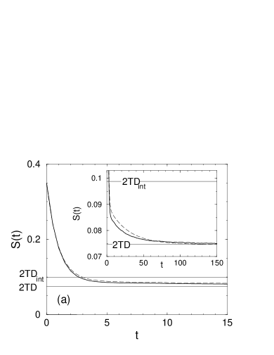
Figure 1: (a) Current-current correlation function $S(t)$ for $T=0.5$, $N_{+}/N_{-}=200/600$ and $m_{\pm}=1\pm 0.3$. In a few collisions $S(t)$ decays down to $2TD_{\mathrm{int}}$ (7). Due to the approximate conservation of $\bar{V}$, it takes much longer (inset) to relax down to $2TD$ (5). Time and distances are measured in units of the average particle spacing $L/(N_{+}+N_{-})$; in this units the typical time between collisions is $\sim\sqrt{m/T}$ for low $T$. A comparison with the analytical approximation (9) and (11) (dashed line) confirms our interpretation that despite the huge mass difference, the proximity to the integrable point is at the origin of the slowly decaying mode. To allow for a better comparison of the numerical data to the analytical approximation, we have multiplied all scattering rates in the latter by a factor of $\approx 2$ to fit the short time scale ((11) is only valid up to prefactors of order 1). (b) Optical conductivity $\mathrm{Re}\,\,\sigma(\omega)$ (same parameters, doubled system size). Weakly violated conservation laws induce a low frequency peak (see inset). The Drude peak $2\pi D\delta(\omega)$ due to momentum conservation (5) is not shown.

In the following, we compare our numerical results for $D$ with the theoretical prediction (1). We first consider the situation $m_{+}\neq m_{-}$, where we expect that only momentum, $P=\sum_{1}^{N_{+}}p_{+,i}+\sum_{1}^{N_{-}}p_{-,i}$, energy $H$ and charges $N_{\pm}$ are conserved. $H$ and $N_{\pm}$ do not contribute to (1) as $\chi_{HJ}=\chi_{N_{\pm}J}=0$ due to symmetry and therefore

$$D = \frac{1}{2}\frac{\chi^{2}_{JP}}{\chi_{PP}}=\frac{1}{2TL}\frac{\langle JP\rangle^{2}}{\langle PP\rangle}=\frac{T(\Delta N)^{2}}{2L}\frac{1}{N_{+}\left\langle p^{2}\right\rangle_{+}+N_{-}\left\langle p^{2}\right\rangle_{-}}$$ (5)

where $N=N_{+}+N_{-}$ and $\Delta N=N_{+}-N_{-}$ are the total number of particles and the total charge, respectively. Conveniently, in our model all static susceptibilities are exactly given by their value in the non-interacting theory as we are considering only local interactions in a classical system, e.g. $\chi_{JP}=\frac{1}{TL}\left(N_{+}\left\langle pv_{+}\right\rangle_{+}-N_{-}\left\langle pv_{-}\right\rangle_{-}\right)$, where the one-particle expectation value $\left\langle...\right\rangle_{\pm}$ in the absence of interactions is given by $\left\langle A\right\rangle_{\pm}=\int dpA(p)e^{-\epsilon_{\pm}(p)/T}/\int dpe^{-\epsilon_{\pm}(p)/T}$.

The situation is qualitatively different when the masses of the “particles” and “holes” are equal, $m_{+}=m_{-}$. The system is integrable and more conserved quantities exist. Jepsen [13] calculated the properties of this system analytically and we used his results [13, 12] for $\sigma(\omega)$ to check our numerics in the non-relativistic limit $T\ll m$. The whole momentum distribution of the particles is conserved for $m_{+}=m_{-}$ since in any collision of particles with equal masses the momentum is just interchanged. Hence, all moments

$$P_{n}=\sum_{i=1}^{N_{+}}p_{+,i}^{n}+\sum_{j=1}^{N_{-}}p^{n}_{-,j}$$ (6)

of the momentum distribution are conserved. What is the projection of $J$ onto the space of CQs? Consider the total velocity $V=\sum_{1}^{N_{+}}v_{+}+\sum_{1}^{N_{-}}v_{-}$ which is conserved for $m_{+}=m_{-}$ and differs from $J$ by just a minus sign. Since for equal masses $\chi_{JP_{n}}=\frac{N_{+}-N_{-}}{TL}\left\langle vp^{n}\right\rangle_{\pm}=\frac{\Delta N}{N}\chi_{VP_{n}}$, the projection $J_{c}$ of $J$ onto the space of conservation laws $P_{n}$ is parallel to $V$ and

$$D_{\mathrm{int}}=\frac{1}{2}\frac{\chi_{JV}^{2}}{\chi_{VV}}=\frac{1}{2TL}\frac{\langle JV\rangle^{2}}{\langle VV\rangle}.$$ (7)

For $m_{+}=m_{-}$, this evaluates to $\frac{1}{2TL}\frac{(\Delta N)^{2}}{N}\left\langle v^{2}\right\rangle_{\pm}$.

Figure 2: (a) The numerically determined Drude weights $D(T)$ both for an integrable model with $m_{+}=m_{-}=1$, (diamonds) and a non-integrable model ($m_{+}=1$, $m_{-}=2.7$) (triangles) agree within the statistical error bars with the theoretical prediction (7) and (5) (thick and thin solid lines) ($N_{+}=3N_{-}$). The dashed line shows the Drude weight (5) of a non-integrable system in the limit $|\Delta m|\to 0^{+}$, $m_{\pm}\approx 1$. (b) Ratio of the fast and slow decay rate $\Gamma_{f}/\Gamma_{s}$ as a function of $\Delta m$ for $m_{\pm}=1\pm\Delta m/2$, $N_{+}/N_{-}=100/300$ and $T=0.25$. Close to the integrable point, the slow decay rate vanishes $\propto(\Delta m)^{2}$. The points are obtained from a fit to $S(t)$ determined from numerical simulations. The analytical result (11,13) (line) describes the observed behavior qualitatively correct. The good agreement at high $\Delta m$ is accidentially, (11) is expected to be valid only for small $\Delta m$ and only up to prefactors of order $1$.

In Fig. 2 we compare the analytical formulas (5) and (7) to our numerical results. Within the statistical errors the computer experiments clearly confirm the theory. The conservation laws for equal masses $m_{+}=m_{-}$ are very different from those for $m_{+}\neq m_{-}$. Therefore, $D$ is not a continuous function of the mass difference $D(\Delta m\to 0)\neq D_{\mathrm{int}}=D(\Delta m=0)$ as is shown in Fig. 2a (dashed line).

What will happen if $\Delta m$ is small? This is a physically relevant situation, e.g. for a Mott insulator with a small gap $\Delta\ll\epsilon_{F}$, where corrections which break the particle-hole symmetry are small but finite. Due to this small mass difference $\Delta m$, the higher moments $P_{n}$ in (6) with $n>1$ will slowly decay and the following physical picture emerges for $|\Delta m|\ll m=(m_{+}+m_{-})/2$: we decompose the current $J=J_{f}+J_{s}$ (as before) into a “fast” component $J_{f}$ perpendicular to the currents $P_{n}$ and the projection $J_{s}$ of $J$ onto the space of slow variables $P_{n}$. After a few collisions, i.e. after the time $t_{f}$, $J_{f}$ has decayed completely and $S(t)=\left\langle J(t)J(0)\right\rangle\approx 2TD_{\mathrm{int}}$ for $t_{f}\ll t\ll t_{s}$ as is shown in Fig. 1a. $J_{s}$ is exactly conserved for $\Delta m=0$. For finite $\Delta m$ the projection $J_{c}$ of $J_{s}=J_{c}+J_{sd}$ onto momentum $P=P_{1}$ is still conserved but the component $J_{sd}$ perpendicular to $P$ decays on the scale $t_{s}\propto 1/(\Delta m)^{2}$. Accordingly, $S(t)$ decays further to $S(t\gg t_{s})=2TD$, where the decay stops (Fig. 1a).

The long-time behavior of $S(t)$ determines the low-frequency behavior of the optical conductivity (Fig. 1b): at zero frequency, $\mathrm{Re}\,\sigma(\omega)$ is characterized by a $\delta$-peak with weight $2\pi D$. For small $\omega$, we expect a sharp peak of width $\Gamma_{s}=1/t_{s}$, weight $2\pi(D_{\mathrm{int}}-D)$ and with a height approximately given by $(D_{\mathrm{int}}-D)/\Gamma_{s}$. The slow decay rate determines $\mathrm{Re}\,\,\sigma(\omega\to 0)$ [2].

In the following, we try to give a crude analytical estimate of the slow decay rate $\Gamma_{s}$ within the framework of the (classical) memory matrix formalism [1]. The correlation function

$$C_{mn}(t)=\langle j_{m}(t)j_{n}(0)\rangle$$ (8)

of a set of currents $j_{0},j_{1},...,j_{N}$ is calculated from

$$(\hat{M}(\omega)\hat{C}^{-1}-i\omega)\hat{C}(\omega)=\hat{C}\quad\mathrm{with}\quad M_{mn}(\omega)=\langle\partial_{t}j_{m}\mid Q\frac{1}{\omega-QLQ}Q\mid\partial_{t}j_{n}\rangle$$ (9)

where $C_{mn}=C(t=0)_{mn}=T\chi_{j_{m}j_{n}}$ is the matrix of susceptibilities, $\hat{M}$ the so-called memory matrix and $L$ the Liouville operator defined by the Poisson brackets with the Hamiltonian $iLA=\{A,H\}$. The time evolution of $\hat{M}$ is determined by the projection of $L$ onto the space perpendicular to the currents $j_{k}$ with the projection operator $Q=1-\sum_{kl}|j_{k}\rangle(\hat{C}^{-1})_{kl}\langle j_{l}|$.

The main idea of the memory matrix formalism is that approximations for $\hat{M}$ are much less “dangerous” than approximations for e.g. $\hat{C}(\omega)$, at least if all relevant slow variables are included in the space of the $j_{n}$. In this case, the dynamics in the perpendicular space defined by $Q$ is dominated by fast processes and therefore $\hat{M}$ is – hopefully – non-singular in the low-frequency limit. Here, we test the applicability of this approach in a situation governed by a clear separation of time scales. It is easy to check [2] that indeed the exact Drude weight (1) is reproduced if all relevant conservation laws are included, e.g. $j_{0}=J$, $j_{n}=P_{n}$, $n=1...\infty$. Actually, it is sufficient to keep track of $J$ and its projections onto the $P_{n}$ and $P$. For $\Delta m=0$, the projection $J_{s}$ of $J$ onto the space of the $P_{n}$ is parallel to $\bar{V}$ with

$$\bar{V}=\sum_{i=1}^{N_{+}+N_{-}}\frac{p_{i}}{\sqrt{m^{2}+p_{i}^{2}}}.$$ (10)

For small $\Delta m$ we replace $m$ by $(m_{+}+m_{-})/2$. We can therefore restrict our analysis to the three-dimensional space of operators $j_{0}=J,j_{1}=P$ and $j_{2}=\bar{V}$. One can check that this approximation is not only valid for $|\Delta m|\ll m$ at any temperature but also for $T\ll m\pm\Delta m$ for arbitrary $\Delta m$ because $J_{s}$ is a linear combination of $P$ and $\bar{V}$ in the latter case.

While the weights of all features in the optical conductivity can be calculated exactly, it is much more difficult to determine the decay rates for small but finite $\Delta m$. To estimate the various elements of the memory matrix, we use two approximations: we neglect all correlations between collisions and we neglect the projection operator $Q$ in (9):

$$M_{nm}(t) \approx \left\langle\partial_{t}j_{n}(t)\partial_{t}j_{m}(0)\right\rangle\approx\sum_{i}\left\langle\Delta j_{n}^{(i)}\Delta j_{m}^{(i)}\delta(t_{i})\right\rangle\delta(t)$$ (11)

$$\approx \frac{N_{+}N_{-}}{L}\left\langle\Delta j_{n}\Delta j_{m}|v_{+}-v_{-}|\right\rangle_{p_{+}p_{-}}\delta(t)$$

where $\Delta j_{n}^{(i)}(p_{+},p_{-})$ is the change of $j_{n}$ at the $i$th collision at time $t_{i}$, $\partial_{t}j_{n}=\sum_{i}\Delta j_{n}^{(i)}\delta(t-t_{i})$ and $\left\langle f_{p_{+},p_{-}}\right\rangle_{p_{+}p_{-}}=\int f_{p_{,}+p_{-}}e^{-(\epsilon_{+}(p_{+})+\epsilon_{-}(p_{-}))/T}/\int e^{-(\epsilon_{+}(p_{+})+\epsilon_{-}(p_{-}))/T}$ is the thermal average over the momenta $p_{\pm}$ of the two incoming particles with velocities $v_{\pm}$ and charge $+$ and $-$, respectively. Note that collisions of particles with equal charge do not change $j_{n}$. Both approximations in (11) are uncontrolled[14] and will induce errors of order $1$ in the prefactors of the collision rates. Nevertheless, a comparison with our numerical data shows that the qualitative dependence of $\sigma$ as a function of $T$, $\Delta m$ and $\Delta N/N$ is very well described by (11). For $N_{+}=N_{-}$ and $\Delta m=0$ and $T\to 0$ we obtain e.g. $\sigma(T)=\sqrt{\pi}/(16\sqrt{mT})$ to be compared to the exact result [12, 13] $\sigma(T)=1/\sqrt{2\pi mT}$, the error is smaller at higher $T$.

The size of $\Delta j_{n}$ determines the various collision rates. $\Delta j_{0}\approx 2(v(p_{+})-v(p_{-}))$ is finite for $\Delta m\to 0$ and $M_{00}$ describes the initial fast decay of $J$. $\Delta j_{1}$ vanishes due to momentum conservation. Accordingly, the projection of $J$ onto $P$ will not decay. $\Delta j_{2}$ is linear in $\Delta m$ as $\bar{V}$ is conserved for $\Delta m=0$ which leads to a slow decay rate proportional to $(\Delta m)^{2}$

$$\Gamma_{s}/\Gamma_{f}\propto(\Delta m)^{2}.$$ (12)

A comparison of the analytical result with the numerical data shows that our analytical calculation within the memory matrix formalism does not only reproduce the exact weights (Fig. 2b) but also describes the relevant decay rates $\Gamma_{s}$ and $\Gamma_{f}$ qualitatively and semi-quantitatively correctly. In Fig. 2b, we compare the exact decay rates determined from a fit to the numerically calculated $S(t)\approx c_{1}e^{-\Gamma_{f}t}+c_{2}e^{-\Gamma_{s}t}+c_{3}$ to the corresponding rates derived from our analytical approximations (9) and (11). In the limit $\Delta m\to 0$ we obtain

$$\Gamma_{s} = \frac{M_{22}-M_{02}^{2}/M_{00}}{C_{22}-C_{12}^{2}/C_{11}},\quad\quad\Gamma_{f}=\frac{M_{00}}{C_{00}(1-(\Delta N/N)^{2})}$$ (13)

where the memory functions $M_{nm}$ are evaluated at $\omega=0$. At low $T$ we get e.g. $\Gamma_{f}\approx 8\sqrt{T/\pi}$ and $\Gamma_{s}\approx 6(\Delta m)^{2}(1-(\Delta N/N)^{2})\sqrt{T/\pi}$.

Within our (crude) approximation scheme, $S(t)$ decays exponentially to a constant for long times. This is certainly not correct, as e.g. for $\Delta m=0$, $S(t)\sim const.-1/t^{\alpha}$ with $\alpha=3$ as is known from the exact result [13, 15]. Our numerical results suggest that the (algebraic) long-time tails are more pronounced for $\Delta m\neq 0$ but we were not able to extract the exponent $\alpha$ reliably due to large finite size effects (due to the hard-core interaction the particles cannot pass each other and their diffusion is stopped after a distance of order $\sqrt{N}$). The main physics discussed in this paper, i.e. the existence of a time-scale $1/\Gamma_{s}\propto 1/(\Delta m)^{2}$, seems not to be affected by the presence of algebraic long-time tails.

How small has $\Delta m$ to be that $\sigma(\omega)$ displays a well defined peak of width $\Gamma_{s}$ due to the slowly decaying component of $J$? To decide this question, we compare $\mathrm{Re}\,\sigma(\omega\to 0^{+},\Delta m\to 0^{+})\approx 2\Delta D_{s}/\Gamma_{s}$ with $\mathrm{Re}\,\sigma(\omega\to 0^{+},\Delta m=0)\approx 2\Delta D_{f}/\Gamma_{f}$ where $\Delta D_{s}=D_{\mathrm{int}}-D$ and $\Delta D_{f}=\chi_{JJ}/2-D_{\mathrm{int}}$ are the weights of the slowly and fast decaying modes, respectively. The low frequency peak is visible if

$$1\gg\frac{\Delta D_{f}}{\Gamma_{f}}/\frac{\Delta D_{s}}{\Gamma_{s}}\approx\frac{(\Delta m)^{2}(1-(\Delta N/N)^{2})^{2}}{2T^{2}(\Delta N/N)^{2}}$$ (14)

where the last equation is valid for low $T$. The peak is not observable for $T\lesssim|\Delta m|$ which is a consequence of the fact that the model is Galileian invariant for $T\to 0$. The slowly decaying modes are much less relevant for $\Delta N=0$, as $\chi_{PJ}=\Delta N/L$ and no well pronounced low-frequency peak develops for low $T$ [3].

In this paper we have investigated numerically and analytically the optical conductivity for a model of charge excitations above a Mott gap. Due to conservation laws, the Drude weight is finite at $T>0$ for $\Delta N\neq 0$. We can confirm predictions (7,5) for the Drude weight and $\sigma(\omega)$ both for an integrable model and in a situation where conservation laws are weakly broken and low-frequency peaks arise in $\sigma(\omega)$. One of the surprises of this study was that even for a really large mass difference, e.g. $m_{\pm}=1\pm 0.3$, the proximity of the Hamiltonian to some integrable point with $m_{+}=m_{-}$ strongly influences the low-frequency conductivity (see Fig. 1b)). At least for the model studied here, the memory matrix formalism is a reliable tool to study this type of physics qualitatively. Furthermore, we expect a quantitative agreement in situations[2] where it is possible to calculate the memory matrix perturbatively. One may speculate that the low-frequency peaks in the optical conductivity of the Bechgaard salts are related to approximate conservation laws as they are characterized by tiny weights, unusual line-shapes and a very long mean-free path[10].

We would like to thank N. Andrei, K. Damle, F. Evers, P. Wölfle and X. Zotos for helpful discussions and the Emmy-Noether program of the DFG for financial support.

References

- [1] \NameForster D. \BookHydrodynamic Fluctuations, Broken Symmetry and Correlation Functions \PublAddison-Wesley, Reading \Year1975.
- [2] \NameRosch A. Andrei N. \REVIEWPhys. Rev. Lett.8520001092.
- [3] \NameRosch A. Andrei N. in preparation.
- [4] \Name Mazur P. \REVIEWPhysica431969533; \NameSuzuki M. \REVIEWPhysica511971277.
- [5] \Name Castella H., Zotos X. Prelovek P. \REVIEWPhys. Rev. Lett.741995972; \Name Fujimoto S. Kawakami N. \REVIEWJ. Phys. A311998465; \Name Zotos X. \REVIEWPhys. Rev. Lett.8219991764.
- [6] \Name Zotos X. , Naef F. Prelovek P. \REVIEWPhys. Rev. B55199711029.
- [7] \Name Zotos X. Prelovek P. \REVIEWPhys. Rev. B531996983.
- [8] \Name Castella H. Zotos X. \REVIEWPhys. Rev. B5419964375.
- [9] \Name Kirchner S. et al. \REVIEWPhys. Rev. B5919991825.
- [10] \NameVescoli V. et al. \REVIEWScience28119981188; \NameSchwartz A. et al. \REVIEWPhys. Rev. B5819981261.
- [11] \Name Giamarchi T. \REVIEWPhys. Rev. B4419912905 and references therein.
- [12] \NameSachdev S. Damle K. \REVIEWPhys. Rev. Lett.781997943; \Name Damle K. Sachdev S. \REVIEWPhys. Rev. B5719988307.
- [13] \Name Jepsen D.W. \REVIEWJ. Math. Phys.61965405.
- [14] The problem arises because the hard-core collisions define a strong coupling problem. In a weak coupling situation[2] the projection can be neglected in lowest order.
- [15] \Name Marro J. Masoliver J. \REVIEWPhys. Rev. Lett.541985731.