International Journal of Modern Physics B,
c  World Scientific Publishing Company

1

ITINERANT AND LOCALIZED STATES

IN STRONGLY CORRELATED SYSTEMS BY A MODIFIED

MEAN-FIELD SLAVE-BOSON APPROACH

EMMANUELE CAPPELLUTI

Dipartimento di Fisica, Università “La Sapienza”, P.le Aldo Moro 2

Roma, 00185, Italy

and INFM, Unità Roma1

The standard mean field slave-boson solution for the infinite-$U$ Hubbard model is revised. A slightly modified version is proposed which includes properly the incoherent contribution of the localized states. In contrast to the standard mean field result, this new proposed solution defines a unique spectral function to be used in the calculation of local and not local quantities, and satisfies the correct thermodynamic relations. The same approach is applied also to the mean field approximation in terms of Hubbard operators. As a byproduct of this analysis, Luttinger’s theorem is shown to be fulfilled in a natural way.

1 Introduction

A paradigmatic model to study systems of strongly correlated electrons is the Hubbard model. It contains the minimum of features necessary to describe bandlike itinerant or localized electrons depending on microscopic parameters. The Hamiltonian has the simple form:

$$H=-\sum_{\sigma}\sum_{ij}t_{ij}c^{\dagger}_{i\sigma}c_{j\sigma}+U\sum_{i}c^{\dagger}_{i\uparrow}c_{i\uparrow}c^{\dagger}_{i\downarrow}c_{j\downarrow},$$ (1)

where the first term is a one-band tight-binding Hamiltonian. Its first kinetic term describes the destruction of an electron on site $j$ and the creation of an electron with the same spin on site $i$. The second term in equation (1) is the on-site repulsion between electrons, which is expected to be relevant in real materials for $d$- and $f$- orbitals. While the limiting case $U\ll t$ can easily be dealt with by means of perturbation theory, leading to a renormalized band of quasiparticles, the intermediate and the strong-coupling limits $U\simeq t$ are much more interesting. From a qualitative point of view, in these regimes the system is described by a narrow coherent band of itinerant quasiparticles on the top of a large background of incoherent localized states. The metal-insulator transition is thus characterized by the disappearing of the coherent band. This picture is confirmed by dynamical mean field analyses^?. In the strong coupling case ($U\gg t$) the bandwidth and the spectral weight of the itinerant quasiparticles scales only with the number of holes $\delta$, so that an insulating state is achieved at half-filling $\delta=0$. In such a situation the total weight of the spectral function is in its incoherent part.

On the analytical ground, all the possible informations about the single-particle properties of the system are obtained by the knowledge of the one-electron Green’s function $G$. Without losing any generality, it can be splitted in a coherent and an incoherent contribution^?:

$$G_{\sigma}({\bf k},\omega)=\frac{Z}{\omega-\epsilon({\bf k})+\mu+i0^{+}\>i{\rm sgn}[\epsilon({\bf k})-\mu]}+G^{{\rm inc}}_{\sigma}({\bf k},\omega),$$ (2)

where $Z$ is the spectral weight of itinerant states with effective dispersion $\epsilon({\bf k})$ and $G^{{\rm inc}}$ contains all the physics not described by the first term. For the above arguments, we expect $Z\propto\delta$.

A meaningful quantity that can be calculated by the Green’s function is the occupation number

$$n_{\sigma}({\bf k})=\int\frac{d\omega}{2\pi i}G_{\sigma}({\bf k},\omega){\rm e}^{-i\omega 0^{-}}.$$ (3)

In a similar way as the Green’s function, $n_{\sigma}({\bf k})$ can be distinguish in a coherent part, with a sharp jump of height $Z$ at the Fermi surface, plus the incoherent background spread over the whole Brillouin zone.

One of the most popular tools to deal with strongly correlated systems is the slave-boson technique^?. Its feasibility makes it suitable to be applied to different models, as for instance the Kondo problem or the Anderson Hamiltonian^?. In the finite $U$ Hubbard model, it is applied by introducing four auxiliary bosonic fields^?, while in the $t$-$J$ Hamiltonian, obtained as strong-coupling limit of the Hubbard one, only one boson is needed. For the purpose of this work we restrict our study to the simplest case of the so-called “$t$-model”, equivalent to the infinite-$U$ Hubbard model or to the $t$-$J$ model with zero exchange coupling constant. In this case the strong correlation arises from the constraint of no double occupancy on each site.

As above discussed, in the $U\rightarrow\infty$ limit the metal-insulator transition, at zero temperature, is driven by only one relevant parameter, the hole number $\delta$, related to the total number of electrons $n$ by $\delta=1-n$. In the mean-field approximation, which represents its simplest formulation, the slave-boson technique maps the strong correlated Hamiltonian into an effective model of non interacting fermions with renormalized bandwidth^?. Thus, the resulting Hamiltonian is thought to describe the physics of the itinerant coherent states, whereas the contribution of the localized states is totally disregarded at this level, and it can be restored only by higher order approximations. In agreement with this picture, the spectral weight associated with the coherent states can be shown to be equal to the doping $\delta$ and it can be therefore identified with $Z$. If one considers the occupation number of the electrons, the mean-field solution of the slave-boson approach accounts only for the sharp jump at the Fermi energy while the incoherent background is missing (figure 1). Incoherent states are described in the slave-boson picture only at higher order than the mean-field solution. An analysis of the finite-$U$ Hubbard model shows that the dynamics of the auxiliary bosons reconstructs the lower and upper Hubbard bands with splitting $\sim U$^?. However in the infinite-$U$ Hubbard model, where single occupancy constraint is more compelling and no energy scale but the kinetic one exists, it is not clear where the incoherent background should be located and how the total sum rule fulfilled. In the $t$-$J$ model, where the inclusion of the exchange term identifies a characteristic magnetic energy, spectral weight is expected to arise on a scale $J$ associated with spin excitations. However, the violation or less of the total sum rule is basically connected with the single occupancy constraint, independently of the exchange term which would just redistribute the total spectral weight. In this perspective, the simple $t$-model is as respresentative as the $t$-$J$ in order to test the conservation of the total spectral weight.

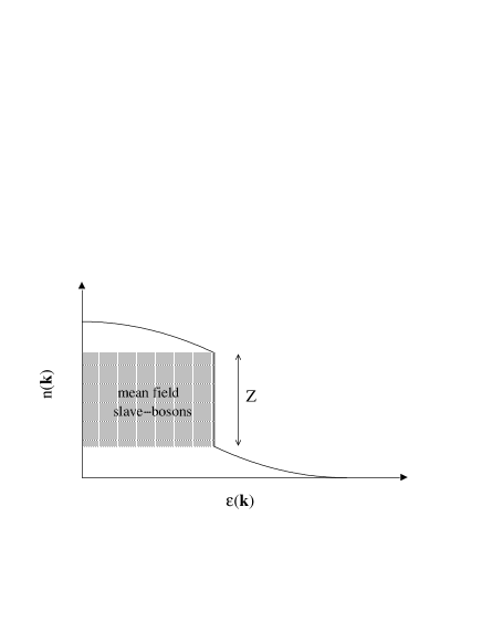
Figure 1: Sketch of the electron occupation number. The shaded area represents the spectral weight of the itinerant quasi-particles as described by the mean-field slave-boson solution.

The aim of this paper is to revise the mean-field solution in order to take into account in a proper way the incoherent background. It is shown that, even in mean-field approximation, a rigorous implementation of the no double occupancy constraint leads to an analytic expression of the Green’s function that describes on the same foot itinerant and localized states. According to its mean-field nature the proposed approach shares with the standard mean-field solution the common shortcomings due to neglecting the boson dynamics. In particular incoherent states in lower and upper bands can not be described. Nevertheless it provides an improved version of the mean-field slave-boson solution free of some inconsistencies of the standard one and preserving the correct spectral weight sum rule. The same procedure is applied to the “mean-field” solution of the $t$-model in terms of Hubbard $X$-operators, which differs deeply from the one obtained by the slave-boson technique. It is shown that the inclusion of the incoherent part permits to overcome some intrinsic inconsistencies of the $X$-operator solution, as for instance about the validity of Luttinger’s theorem.

2 Mean field approximation in the slave-boson approach

Let us start with a brief summary of the well-known mean field solution within the slave-boson formalism^?. This reviewing is finalized to present all the main analytic steps of such a derivation permitting to point out the critical passages that will be afterwards modified in order to obtain a consistent picture.

Let us consider the Hamiltonian of the $t$-model:

$$H=\sum_{i\neq j,\sigma}t_{ij}\tilde{c}^{\dagger}_{i\sigma}\tilde{c}_{j\sigma}-\mu\sum_{i,\sigma}\tilde{c}^{\dagger}_{i\sigma}\tilde{c}_{i\sigma},$$ (4)

where $\tilde{c}$, $\tilde{c}^{\dagger}$ are electronic fields operating on the reduced Hilbert space with no double occupied sites.

In the slave-boson formalism the creation (destruction) operator of the real electron is decomposed in two operators by the usual substitution:

$$\tilde{c}^{\dagger}_{i\sigma} \longrightarrow b_{i}f^{\dagger}_{i\sigma},$$ (5)

$$\tilde{c}_{i\sigma} \longrightarrow b^{\dagger}_{i}f_{i\sigma},$$ (6)

where the $b$ and $f$ operators fulfil respectively bosonic and fermionic algebras. The constraint of no double occupancy is implemented on each site by the condition

$$b^{\dagger}_{i}b_{i}+f^{\dagger}_{i\uparrow}f_{i\uparrow}+f^{\dagger}_{i\downarrow}f_{i\downarrow}=1.$$ (7)

By using the relations (5)-(6), and introducing the Lagrange multiplier $\lambda_{i}$ on each site to enforce the constraint, the slave-boson Hamiltonian reads:

$$H=\sum_{i\neq j,\sigma}t_{ij}b_{i}b^{\dagger}_{j}f^{\dagger}_{i\sigma}f_{j\sigma}-\mu\sum_{i,\sigma}f^{\dagger}_{i\sigma}f_{i\sigma}+\sum_{i}\lambda_{i}\left[b^{\dagger}_{i}b_{i}+f^{\dagger}_{i\uparrow}f_{i\uparrow}+f^{\dagger}_{i\downarrow}f_{i\downarrow}-1\right].$$ (8)

In the derivation of equation (8) the relation

$$\tilde{c}^{\dagger}_{i\sigma}\tilde{c}_{i\sigma}=b_{i}b^{\dagger}_{i}f^{\dagger}_{i\sigma}f_{i\sigma}=f^{\dagger}_{i\sigma}f_{i\sigma}$$ (9)

has been used.

In the mean-field approximation the local fields $b_{i}(t)$, $b^{\dagger}_{i}(t)$, $\lambda_{i}(t)$ are replaced by their mean-field global values: $b_{i}(t)\rightarrow\langle b_{i}\rangle\equiv b$, $b^{\dagger}_{i}(t)\rightarrow\langle b^{\dagger}_{i}\rangle\equiv b^{*}$, $\lambda_{i}(t)\rightarrow\langle\lambda_{i}\rangle\equiv\lambda$. Note that in such an approximation both the space and time dependences of $b$ and $\lambda$ are dropped. The resulting Hamiltonian describes an effective model of renormalized non interacting fermions:

$$H^{MF}=\sum_{i\neq j,\sigma}b^{2}t_{ij}f^{\dagger}_{i\sigma}f_{j\sigma}-(\mu-\lambda)\sum_{i,\sigma}f^{\dagger}_{i\sigma}f_{i\sigma}+\lambda\sum_{i}\left[b^{2}-1\right],$$ (10)

or, in Fourier space,

$$H^{MF}=\sum_{{\bf k},\sigma}\left[b^{2}t({\bf k})-\mu+\lambda\right]f^{\dagger}_{{\bf k}\sigma}f_{{\bf k}\sigma}+\lambda\left[b^{2}-1\right].$$ (11)

The Green’s function of the $f$-fermions takes the simple form

$$G^{f}_{\sigma}({\bf k};\omega)=\frac{1}{\omega-b^{2}t({\bf k})+\mu-\lambda+\>i{\rm sgn}[b^{2}t({\bf k})-\mu+\lambda]},$$ (12)

that represents the Green’s function of purely itinerant fermions with bandwidth renormalized by a factor $b^{2}$ and chemical potential shifted by $-\lambda$. The corresponding zero temperature occupation number of the $f$-particles,

$$n^{f}_{\sigma}({\bf k})=\int\frac{d\omega}{2\pi i}G^{f}_{\sigma}({\bf k},\omega){\rm e}^{-i\omega 0^{-}},$$ (13)

has thus a jump from 1 to 0 at the chemical potential. For simplicity in the following the zero temperature case will be always considered. Discussion and results can be however straightforwardly generalized at finite temperature.

The internal energy can be expressed as function of $n^{f}_{\sigma}({\bf k})$:

$$E=\sum_{{\bf k},\sigma}\left[b^{2}t({\bf k})-\mu+\lambda\right]n^{f}_{\sigma}({\bf k})+\lambda\left[b^{2}-1\right].$$ (14)

The physical solution for the mean-field parameters $b^{2}$ and $\lambda$ is obtained by minimizing equation (14). Their analytical expressions are:

$$\lambda=-\sum_{{\bf k},\sigma}t({\bf k})n^{f}_{\sigma}({\bf k}),$$ (15)

and

$$b^{2}=1-\sum_{{\bf k},\sigma}n^{f}_{\sigma}({\bf k}).$$ (16)

By using these relations, equation (14) is therefore simplified:

$$E=\sum_{{\bf k},\sigma}b^{2}t({\bf k})n^{f}_{\sigma}({\bf k})-\mu\sum_{{\bf k},\sigma}n^{f}_{\sigma}({\bf k}).$$ (17)

The total number of electrons $n$ is easily obtained by the thermodynamic relation $n=-\partial E/\partial\mu$:

$$n=n^{f}=\sum_{{\bf k},\sigma}n^{f}_{\sigma}({\bf k}),$$ (18)

which identifies the number of “real” electrons with the number of the $f$-fermions, that is to say with the number of single occupied states.

Equation (18) is indeed consistent with relation (9). However, some intrinsic inconsistencies appear just by looking at the spectral function. If one considers the Green’s function of real electrons

$$G_{\sigma}(i,j;t)=-i\langle T_{t}c_{i\sigma}(t)c^{\dagger}_{j\sigma}\rangle,$$ (19)

the relation between $G_{\sigma}$ and $G^{f}_{\sigma}$, within the mean field approximation, is simply:

$$G_{\sigma}(i,j;t)=b^{2}G^{f}_{\sigma}(i,j;t).$$ (20)

The same relation thus holds for the spectral functions $A({\bf k},\omega)=b^{2}A^{f}({\bf k},\omega)$, and for the corresponding electronic occupation number

$$n({\bf k})=b^{2}n^{f}({\bf k}).$$ (21)

This result is in partial agreement with the physical situation depicted in figure 1, where the contribution of the coherent states to the total number of electrons scales with $Z=\delta=1-n$, but it is in open contrast with Equation (18). In order to reconcile the two descriptions one should assume two relations linking $n({\bf k})$ with $n^{f}({\bf k})$, respectively $n({\bf k})=n^{f}({\bf k})$ and $n({\bf k})=b^{2}n^{f}({\bf k})$. The first one should be employed to calculate only local quantities as the total number of electrons $n$, as it has implicitly done in the expression of the internal energy in equation (17). The second one should be used for non local quantities, as shown by the kinetic energy in the same equation. It is not clear in this procedure which of them is the physical occupation number of the real electrons.

The inconsistency is clearly related to the neglecting of the incoherent background of localized states. The spectral function $A({\bf k},\omega)$ as well as the occupation number $n({\bf k})$ of the real electrons should contain both the coherent and incoherent contributions. In the following it is shown how the previous approach can be modified to take into account in a simply way both the coherent and incoherent parts, leading to an unambiguous determination of the spectral function and of the related quantities $n({\bf k})$ and $n$.

3 Modified mean-field approach

Actually, the procedure here proposed is quite simple. The basilar consideration arises from the realizing that the above discrepancies stem from the different implementations of the no double occupancy constraint. Indeed, in the evaluation of the local quantity $\tilde{c}^{\dagger}_{i\sigma}\tilde{c}_{i\sigma}$ the condition (9) has been used to identity $\langle\tilde{c}^{\dagger}_{i\sigma}\tilde{c}_{i\sigma}\rangle$ with $\langle f^{\dagger}_{i\sigma}f_{i\sigma}\rangle$. A similar equality however does not hold for the non local Green’s function of the real electrons defined in equation (19). In this situation equation (9) can not be applied whereas the relation (20) is rather fulfilled. An appropriate way to deal with the generic Green’s function is to split it in the local and non local part:

$$G_{\sigma}(i,j;t)=-i\langle T_{t}\tilde{c}_{i\sigma}(t)\tilde{c}^{\dagger}_{j\sigma}\rangle\left[1-\delta_{ij}\right]-i\langle T_{t}\tilde{c}_{i\sigma}(t)\tilde{c}^{\dagger}_{i\sigma}\rangle\delta_{ij}.$$ (22)

Let us now introduce the slave-boson formalism and perform the mean field approximation in two steps: firstly the fields $b_{i}(t)$, $b^{\dagger}_{i}(t)$ are replaced by their mean field values with respect to the time $b_{i}(t)\rightarrow b_{i}$, $b^{\dagger}_{i}(t)\rightarrow b^{\dagger}_{i}$. Note that they still preserve a full site dependence. As a consequence of this first approximation the relation (9) can now be formulated in the dynamic version:

$$\tilde{c}^{\dagger}_{i\sigma}(t)\tilde{c}_{i\sigma}=b_{i}b^{\dagger}_{i}f^{\dagger}_{i\sigma}(t)f_{i\sigma}=f^{\dagger}_{i\sigma}(t)f_{i\sigma}.$$ (23)

We can now safely apply in equation (22) the spatial mean field approximation in the first non local part, while in the second local term the relation (23) can correctly be employed. The resulting Green’s function becomes:

$$G_{\sigma}(i,j;t)=-ib^{2}\langle T_{t}f_{i\sigma}(t)f^{\dagger}_{j\sigma}\rangle\left[1-\delta_{ij}\right]-i\langle T_{t}f_{i\sigma}(t)f^{\dagger}_{i\sigma}\rangle\delta_{ij},$$ (24)

or, in a more compact way,

$$G_{\sigma}(i,j;t)=-ib^{2}\langle T_{t}f_{i\sigma}(t)f^{\dagger}_{j\sigma}\rangle-i\left[1-b^{2}\right]\langle T_{t}f_{i\sigma}(t)f^{\dagger}_{i\sigma}\rangle\delta_{ij}.$$ (25)

In Fourier space, the analytic expression of the electronic Green’s function takes the form:

$$G_{\sigma}({\bf k};\omega)=ZG^{f}_{\sigma}({\bf k};\omega)+\left(1-Z\right)\sum_{{\bf k}}G_{\sigma}({\bf k};\omega),$$ (26)

where $Z$ is the coherent spectral weight $Z=b^{2}$. A straightforward consequence of equation (26) is:

$$\sum_{{\bf k}}G_{\sigma}({\bf k};\omega)=\sum_{{\bf k}}G^{f}_{\sigma}({\bf k};\omega),$$ (27)

so that the electronic propagator $G$ can be fully expressed as function of $G^{f}$:

$$G_{\sigma}({\bf k};\omega)=ZG^{f}_{\sigma}({\bf k};\omega)+\left(1-Z\right)\sum_{{\bf k}}G^{f}_{\sigma}({\bf k};\omega).$$ (28)

From equation (26), the occupation number of the real electrons is also immediately evaluated:

$$n_{\sigma}({\bf k})=Zn^{f}_{\sigma}({\bf k})+\left(1-Z\right)n_{\sigma},$$ (29)

where $n_{\sigma}$ is the total number of electrons per spin.

The analytic expressions of the Green’s function for the $f$-fermions, and consequently of $n^{f}_{\sigma}({\bf k})$, in the present approach are just the same as in the standard mean field slave-boson result given by equation (12). This can be easily checked by considering that the mean field Hamiltonian in term of $f$-operators, as defined in equation (10), is still valid in the present approach.

In agreement with the intuitive picture, the occupation number derived in the present paper contains two contributions: one describing itinerant dispersive states with total spectral weight $Z$ and accounting for the sharp jump at the Fermi energy; and an incoherent part of localized states with no ${\bf k}$-dependence and containing $(1-Z)n$ spectral weight. The resulting picture is shown in figure 2.

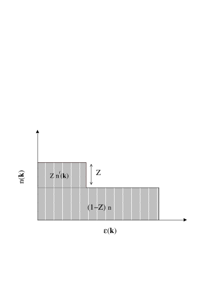
Figure 2: Occupation number of real electrons as calculated by equation (29). It is composed by a coherent part with $Zn^{f}$ states and an incoherent one with $(1-Z)n$ states.

It should be stressed that equation (28) defines in an unambiguous way the Green’s function of real electrons $G$, although expressed as function of $G^{f}$. It can be now directly employed to calculate any quantity involving one-particle physics, with no more need to deal with auxiliary fields. In particular, this unique definition of $G$, and consequently of $n({\bf k})$, yields a consistent derivation of the total number of electrons and of the internal energy, overcoming the discrepancy found in the standard mean field slave-boson solution.

By working directly in $\tilde{c}$-operators, the total number of electrons $n$ and the internal energy $E$ are expressed as function of $n_{\sigma}({\bf k})$ as:

$$n=\sum_{{\bf k},\sigma}\langle\tilde{c}^{\dagger}_{{\bf k},\sigma}\tilde{c}_{{\bf k},\sigma}\rangle=\sum_{{\bf k},\sigma}n_{\sigma}({\bf k}),$$ (30)

$$E=\sum_{{\bf k},\sigma}\left[t({\bf k})-\mu\right]\langle\tilde{c}^{\dagger}_{{\bf k},\sigma}\tilde{c}_{{\bf k},\sigma}\rangle=\sum_{{\bf k},\sigma}\left[t({\bf k})-\mu\right]n_{\sigma}({\bf k}).$$ (31)

Inserting equation (29) in (30) we then obtain

$$n=\sum_{{\bf k},\sigma}n^{f}_{\sigma}({\bf k}).$$ (32)

On the other hand, as previously discussed, the number of particles can be derived also by the thermodynamic relation $n=-\partial E/\partial\mu$. The internal energy, by using the same expression of $n_{\sigma}({\bf k})$ as in the calculation of $n$, reads:

$$E=\sum_{{\bf k},\sigma}\left[b^{2}t({\bf k})-\mu\right]n^{f}_{\sigma}({\bf k}).$$ (33)

In the same way as in the standard mean field slave-boson derivation, the physical values of $b^{2}$ and $\lambda$ that appear as parameters in $n^{f}_{\sigma}({\bf k})$ are found:

$$\lambda=-\sum_{{\bf k},\sigma}t({\bf k})n^{f}_{\sigma}({\bf k}),$$ (34)

$$b^{2}=1-\sum_{{\bf k},\sigma}n^{f}_{\sigma}({\bf k}).$$ (35)

Then, deriving $E$ with respect to $\mu$ as required by the thermodynamic relation, one finally obtains

$$n=\sum_{{\bf k},\sigma}n^{f}_{\sigma}({\bf k}),$$ (36)

just like in equation (32).

This result shows the fully consistency of the analytic expression of $G$ derived in the present approach. The Green’s function for real electrons is univocally determined and its employment to calculate the total number of electrons and the internal energy obeys the thermodynamic relation $\partial E/\partial\mu=-n$. It is also worthy to note that Luttinger’s theorem is naturally fulfilled by using the Green’s function here derived. This is particularly interesting since the validity of Luttinger’s theorem has not been imposed as a precondition to be satisfied. This will appear even more relevant if compared with the results of mean field theories performed within the $X$-operator formalism, where not only the thermodynamic relation $\partial E/\partial\mu=-n$ is not fulfilled, but the validity or the breakdown of Luttinger’s theorem is controversial. In the next section it will be shown how the inclusion of the incoherent background, in the same spirit of the present analysis, allows to overcome all these inconsistencies also in the mean field solutions based on the Hubbard $X$-operators.

4 Hubbard operators and mean field theories

One of the advantages of using $X$-operators is that they permit to work directly in terms of real electrons, without introducing any auxiliary field. In the case of the $t$-model here considered, the $X$-operators live in the reduced Hilbert space constructed on each site by the states $|0\rangle$, $|\uparrow\rangle$, $|\downarrow\rangle$. The Hubbard $X$-operators can then be represented as projection operators: $X^{\alpha\beta}=|\alpha\rangle\langle\beta|$. It is easy to check that they follow the algebra:

$$\left[X^{\alpha\beta}_{i},X^{\gamma\delta}_{j}\right]_{\pm}=\delta_{ij}\left(\delta_{\beta\gamma}X^{\alpha\delta}_{i}\pm\delta_{\alpha\delta}X^{\gamma\beta}_{i}\right).$$ (37)

Moreover the more restrictive relation

$$X^{\alpha\beta}X^{\gamma\delta}=\delta_{\beta\gamma}X^{\alpha\delta}$$ (38)

is obeyed.

By using the Hubbard operator formalism, the $t$-model Hamiltonian can be written as:

$$H=\sum_{i\neq j,\sigma}t_{ij}X^{\sigma 0}_{i}X^{0\sigma}_{j}-\mu\sum_{i,\sigma}X^{\sigma\sigma}_{i}.$$ (39)

In similar way, the Green’s function of real electrons is defined as:

$$G_{\sigma}(i,j;t)=-i\langle T_{t}X^{0\sigma}_{i}(t)X^{\sigma 0}_{j}\rangle.$$ (40)

Different mean field approximations in terms of Hubbard $X$-operators have been performed in literature by using several approaches: diagrammatic studies^?,? as well as derivations based on the equation of motion^?. All these analyses converge to a unique expression of the mean field Green’s function:

$$G_{\sigma}({\bf k};\omega)=\frac{Z}{\omega-Zt({\bf k})+\mu-\lambda+\>i{\rm sgn}[Zt({\bf k})-\mu+\lambda]},$$ (41)

where, unlike in the slave-boson technique,

$$Z=1-\frac{n}{2},$$ (42)

and

$$\lambda=-\frac{1}{2}\sum_{{\bf k},\sigma}t({\bf k})n^{f}_{\sigma}({\bf k}).$$ (43)

Coherently with the spirit of a mean field approximation, equation (41) describes a system of non interacting electrons with total spectral weight $(1-n/2)$ and with a dispersive band renormalized by the same factor.

The occupation number is directly evaluated by (41). In fact, equation (38) implies as a particular case the relation

$$X^{\sigma\sigma}_{i}=X^{\sigma 0}_{i}X^{0\sigma}_{i},$$ (44)

hence

$$n_{\sigma}({\bf k})=\left(1-\frac{n}{2}\right)\Theta\left[\mu-\left(1-n/2\right)t({\bf k})-\lambda\right],$$ (45)

where $\Theta$ is the Heaviside function. The corresponding total number of electrons,

$$n=\left(1-\frac{n}{2}\right)\sum_{{\bf k},\sigma}n_{\sigma}({\bf k}),$$ (46)

shows one the peculiarities of the mean field solutions based on $X$-operators, namely the breakdown of Luttinger’s theorem. In fact, according to equation (46), the half-filled case $n=1$ corresponds to the complete filling of the electronic band and to a vanishing Fermi surface. On the contrary, the half-band filling case corresponds to $n=2/3$ leading to unphysical results. For instance, all the properties and instabilities of the system due to possible nesting of the Fermi surface, as antiferromagnetic or charge-density-wave ordering, lie around this particular value $n=2/3$, a clear artifact of the approximation.

On the other hand, the same breakdown of Luttinger’s theorem appears questionable. One could as well use the above widely discussed thermodynamic relation $\partial E/\partial\mu=-n$ to determine the total number of electrons. However, it is easy to check that the expression (45), once plugged in the internal energy

$$E=\sum_{i\neq j,\sigma}\left[t_{ij}-\mu\delta_{ij}\right]\langle X^{\sigma 0}_{i}X^{0\sigma}_{j}\rangle=\sum_{{\bf k},\sigma}\left[t({\bf k})-\mu\right]n_{\sigma}({\bf k}),$$ (47)

does not reproduce the result of equation (46).

We found ourselves in the same controversial situation as for the slave-boson solution. As before, one should postulate that the electronic propagator in equation (41) (and related functions like spectral function or occupation number $n_{\sigma}({\bf k})$) has to be used only for non local quantities as the kinetic energy, but it does not give any information about the total number of particles. This inconsistency was in that case solved by the introduction of the incoherent background. An identical result will be also recovered in the Hubbard operator approach.

Let us rewrite the “correct” occupation number by adding an incoherent contribution $B$:

$$n_{\sigma}({\bf k})=\left(1-\frac{n}{2}\right)\Theta\left[\mu-\left(1-n/2\right)t({\bf k})-\lambda\right]+B.$$ (48)

The total number of electrons is thus given by:

$$n=\left(1-\frac{n}{2}\right)\sum_{{\bf k},\sigma}\Theta\left[\mu-\left(1-n/2\right)t({\bf k})-\lambda\right]+2B.$$ (49)

By substituting equation (48) in (47), the internal energy becomes:

$$E=\left(1-\frac{n}{2}\right)\sum_{{\bf k},\sigma}t({\bf k})\Theta\left[\mu-\left(1-n/2\right)t({\bf k})-\lambda\right]-\mu n.$$ (50)

The thermodynamic relation can now be employed to determine the spectral weight of the incoherent background $B$ by requiring the total number of electrons to be equal to equation (49). The derivative of the internal energy in equation (50) with respect to $\mu$ gives

$$\frac{\partial E}{\partial\mu}=-n=\frac{\partial n}{\partial\mu}\lambda-n-\mu\frac{\partial n}{\partial\mu}+\left(\mu-\lambda\right)\frac{\partial}{\partial\mu}\sum_{{\bf k},\sigma}\Theta\left[\mu-\left(1-n/2\right)t({\bf k})-\lambda\right],$$ (51)

where the equality

$$\left(1-\frac{n}{2}\right)t({\bf k})\frac{\partial}{\partial\mu}\Theta\left[\mu-\left(1-n/2\right)t({\bf k})-\lambda\right]=\left(\mu-\lambda\right)\frac{\partial}{\partial\mu}\Theta\left[\mu-\left(1-n/2\right)t({\bf k})-\lambda\right]$$ (52)

has been used. Equation (51) can be further simplified to obtain

$$\frac{\partial n}{\partial\mu}=\frac{\partial}{\partial\mu}\sum_{{\bf k},\sigma}\Theta\left[\mu-\left(1-n/2\right)t({\bf k})-\lambda\right],$$ (53)

whose solution is trivially:

$$n=\sum_{{\bf k},\sigma}\Theta\left[\mu-\left(1-n/2\right)t({\bf k})-\lambda\right].$$ (54)

The constant $B$ is thus easily obtained by equating (49) with (54):

$$B=\frac{n^{2}}{4}.$$ (55)

Note that the validity of Luttinger’s theorem is now unambiguously defined and, just as in the slave-boson formalism, arises in a natural way from the correct $n_{\sigma}({\bf k})$ which includes the proper incoherent background.

5 Summary and discussion

A slightly modified version of the slave-boson mean field approximation has been proposed in this paper to account for the localized incoherent background missing in the standard mean field theories. In contrast to them, the resulting Green’s function here derived can be safely used in the calculation of any, local or non local, quantity as the kinetic energy, the total number of electrons or the internal energy. It has also been shown that Luttinger’s theorem is naturally fulfilled when such a Green’s function is employed.

This approach permits a particular compact and suitable way, although approximate, to deal with the redistribution of the one-particle spectral weight due to strong correlation effects. Broken symmetry states, at a mean field level, can be also taken into account in similar way. A straightforward generalization is the superconducting case. It is well known that no purely local $s$-wave Cooper pair can be established in a strongly correlated system, once an attractive interaction is taken into account, because of the forbidding of double occupancy. However, a common shortcoming of the standard mean field theories is to allow for a finite local $s$-wave order parameter as a consequence of the relaxing of the local constraint^?. This spurious result disappears when the modified mean field approximation here proposed is used. Just in the same way as in the normal state, the anomalous propagator $F(ij;t)=-i\langle\tilde{c}^{\dagger}_{i\uparrow}(t)\tilde{c}^{\dagger}_{j\downarrow}\rangle$ can be splitted in a local and non local part. Following the previous procedure, it easy to obtain the corresponding BCS expression for the anomalous Green’s function $F$:

$$F({\bf k};\omega)=-Z\frac{\Delta({\bf k})}{\omega^{2}-\xi^{2}({\bf k})-\Delta^{2}({\bf k})}+Z\sum_{{\bf k}}\frac{\Delta({\bf k})}{\omega^{2}-\xi^{2}({\bf k})-\Delta^{2}({\bf k})}.$$ (56)

Note that both the local part has the same spectral weight $Z=b^{2}$ as the non local one because the relation (9) can not be employed in this case. and the non local part have the same spectral weight. From equation (56) it is thus clear that the condensate relative to local Cooper pairs, given by the order parameter $\sum_{{\bf k}}F({\bf k};\omega)$, is identically zero, as physically expected.

Acknowledgements

The author would like to thank R. Zeyher and M. Grilli for the useful discussions.

References

- [1] For a review see: A. Georges, G. Kotliar, W. Krauth, M.J. Rozenberg, Rev. Mod. Phys. 68, 13 (1996).
- [2] A.A. Abrikosov, L.P. Gorkov and I.E. Dzyaloshinski, Methods of Quantum Field Theory in Statistical Physics, (Dover, New York, 1975).
- [3] P. Coleman, Phys. Rev. B29, 3035 (1987).
- [4] G. Bickers, Rev. Mod. Phys. 59, 845 (1987).
- [5] G. Kotliar, A.E. Ruckenstein, Phys. Rev. Lett. 57, 1362 (1986).
- [6] G. Kotliar, J. Liu, Phys. Rev. Lett. 61, 1784 (1988).
- [7] R. Raimondi and C. Castellani, Phys. Rev. B48, 11453 (1993).
- [8] Yu A. Izyumov, B.M. Letfulov, J. Phys.: Condens. Matter 2, 8905 (1990).
- [9] I.S. Sandalov, M. Richter, Phys. Rev. B50, 12855 (1994).
- [10] N.M. Plakida, V.Yu. Yushankhai, I.V. Stasyuk, Physica C160, 80 (1989).