Density of states, Potts zeros, and Fisher zeros of the $Q$-state Potts model for continuous $Q$

Abstract

The $Q$-state Potts model can be extended to non-integer and even complex $Q$ by expressing the partition function in the Fortuin-Kasteleyn (F-K) representation. In the F-K representation the partition function, $Z(Q,a)$, is a polynomial in $Q$ and $v=a-1$ ($a=e^{\beta J}$) and the coefficients of this polynomial, $\Phi(b,c)$, are the number of graphs on the lattice consisting of $b$ bonds and $c$ connected clusters. We introduce the random-cluster transfer matrix to compute $\Phi(b,c)$ exactly on finite square lattices with several types of boundary conditions. Given the F-K representation of the partition function we begin by studying the critical Potts model $Z_{CP}=Z(Q,a_{c}(Q))$, where $a_{c}(Q)=1+\sqrt{Q}$. We find a set of zeros in the complex $w=\sqrt{Q}$ plane that map to (or close to) the Beraha numbers for real positive $Q$. We also identify $\tilde{Q}_{c}(L)$, the value of $Q$ for a lattice of width $L$ above which the locus of zeros in the complex $p=v/\sqrt{Q}$ plane lies on the unit circle. By finite-size scaling we find that $1/\tilde{Q}_{c}(L)\to 0$ as $L\to\infty$. We then study zeros of the antiferromagnetic (AF) Potts model in the complex $Q$ plane and determine $Q_{c}(a)$, the largest value of $Q$ for a fixed value of $a$ below which there is AF order. We find excellent agreement with Baxter’s conjecture $Q_{c}^{AF}(a)=(1-a)(a+3)$. We also investigate the locus of zeros of the ferromagnetic Potts model in the complex $Q$ plane and confirm that $Q_{c}^{FM}(a)=(a-1)^{2}$. We show that the edge singularity in the complex $Q$ plane approaches $Q_{c}$ as $Q_{c}(L)\sim Q_{c}+AL^{-y_{q}}$, and determine the scaling exponent $y_{q}$ for several values of $Q$. Finally, by finite size scaling of the Fisher zeros near the antiferromagnetic critical point we determine the thermal exponent $y_{t}$ as a function of $Q$ in the range $2\leq Q\leq 3$. Using data for lattices of size $3\leq L\leq 8$ we find that $y_{t}$ is a smooth function of $Q$ and is well fit by $y_{t}={1+Au+Bu^{2}\over C+Du}$ where $u=-{2\over\pi}\cos^{-1}{\sqrt{Q}\over 2}$. For $Q=3$ we find $y_{t}\simeq 0.6$; however if we include lattices up to $L=12$ we find $y_{t}\simeq 0.50(8)$ in rough agreement with a recent result of Ferreira and Sokal $[$J. Stat. Phys. 96, 461 (1999)$]$.

PACS number(s): 05.10.$-$a, 05.50.+q, 64.60.Cn, 75.10.Hk

I introduction

The $Q$-state Potts model[1] in two dimensions exhibits a rich variety of critical behavior and is very fertile ground for the analytical and numerical investigation of first- and second-order phase transitions. With the exception of the $Q=2$ Potts (Ising) model in the absence of an external magnetic field, exact solutions for arbitrary $Q$ are not known. However, some exact results at the critical temperature have been established for the $Q$-state Potts model. From the duality relation the ferromagnetic critical temperature is known to be $T_{c}=J/k_{B}{\rm ln}(1+\sqrt{Q})$ for the isotropic square lattice. Baxter[2] calculated the free energy at $T_{c}$ in the thermodynamic limit, and showed that the Potts model has a second-order phase transition for $Q\leq 4$ and a first-order transition for $Q>4$. The critical exponents for the ferromagnetic Potts model are well known[3, 4, 5].

On the other hand, the antiferromagnetic Potts model is much less well understood than the ferromagnetic model. Recently the three-state Potts antiferromagnet on the square lattice has attracted a good deal of interest[6, 7, 8, 9, 10, 11, 12, 13, 14, 15, 16, 17, 18, 19, 20, 21, 22, 23, 24, 25, 26]. Baxter[10] conjectured that the critical point of the Potts antiferromagnet on the square lattice is given by $T_{c}=J/k_{B}{\rm ln}(\sqrt{4-Q}-1)$, and evaluated the critical free energy and internal energy. The Baxter formula for the critical temperature gives the known exact value for $Q=2$, a critical point at zero temperature for $Q=3$, and no critical point for $Q>3$. For continuous $Q$ in the range $0<Q<3$, Kim et al.[27] have studied the antiferromagnetic Potts critical point through the zeros of the partition function and found good agreement with the Baxter formula. With the exception of the Ising model, the critical exponents of the Potts antiferromagnets are not known. However, for $Q=3$ the ratio of critical exponents $\gamma/\nu$ is known to be 5/3[16, 17].

By introducing the concept of the zeros of the partition function in the complex magnetic-field plane (Yang-Lee zeros), Yang and Lee[28] proposed a mechanism for the occurrence of phase transitions in the thermodynamic limit and yielded a new insight into the unsolved problem of the Ising model in an arbitrary nonzero external magnetic field. It has been shown[28, 29, 30] that the distribution of the zeros of a model determines its critical behavior. Lee and Yang[28] also formulated the celebrated circle theorem which states that the Yang-Lee zeros of the Ising ferromagnet lie on the unit circle in the complex magnetic-field ($x=e^{\beta h}$) plane. However, for the $Q$-state Potts model with $Q>2$ the Yang-Lee zeros lie close to, but not on, the unit circle with the two exceptions of the critical point $x=1$ ($h=0$) itself and the zeros in the limit $T=0$[31].

Fisher[32] emphasized that the partition function zeros in the complex temperature plane (Fisher zeros) are also very useful in understanding phase transitions, and showed that for the square lattice Ising model in the absence of an external magnetic field the Fisher zeros lie on two circles in the thermodynamic limit. In particular, using the Fisher zeros both the ferromagnetic phase and the antiferromagnetic phase can be considered at the same time. The critical behavior of the Potts model in both the ferromagnetic and antiferromagnetic phases have been studied using the distribution of the Fisher zeros, and the Baxter conjecture for the antiferromagnetic critical temperature has been verified[27]. Recently the Fisher zeros of the $Q$-state Potts model on square lattices have been studied extensively for integer $Q>2$[33, 34, 35, 36, 37, 38, 39, 40, 41, 42, 43, 44, 45, 46] and noninteger $Q$[27]. Exact numerical studies have shown[27, 35, 36, 40, 41, 43, 44, 46] that for self-dual boundary conditions the Fisher zeros of the $Q>1$ Potts models on a finite square lattice are located on the unit circle in the complex $p$ plane for ${\rm Re}(p)>0$, where $p=(e^{\beta J}-1)/\sqrt{Q}$. It has been analytically shown that all the Fisher zeros of the infinite-state Potts model lie on the unit circle for any size of square lattice with self-dual boundary conditions[42], and the Fisher zeros near the ferromagnetic critical point of the $Q>4$ Potts models on the square lattice lie on the unit circle in the thermodynamic limit[45]. Chen et al.[41] conjectured that when $Q$ reaches a certain critical value $\tilde{Q}_{c}(L)$, all Fisher zeros for $L\times L$ square lattices with self-dual boundary conditions are located at the unit circle $|p|=1$. In this paper we verify this conjecture and find that $\tilde{Q}_{c}(L)$ approaches infinity in the thermodynamic limit, and we study the thermal exponent $y_{t}$ of the square-lattice Potts antiferromagnet using the Fisher zeros near the antiferromagnetic critical point.

In this paper we also discuss the partition function zeros in the complex $Q$ plane (Potts zeros) of the $Q$-state Potts model. The Potts zeros at $\beta J=-\infty$ have been investigated extensively to understand the ground states of the antiferromagnetic Potts model and the chromatic polynomial in graph theory[23, 26, 47, 48, 49, 50, 51]. Recently the Potts zeros at finite temperatures have been studied for cyclic ladder graphs and $e^{\beta J}\leq 1$[50].

In the next section we describe two algorithms to evaluate the density of states, from which the exact partition function of the $Q$-state Potts model is obtained. The first algorithm (microcanonical transfer matrix) is applied to only integer $Q$ but allows us to calculate the density of states for relatively larger lattices, while the second algorithm (random-cluster transfer matrix) gives the density of states for any value of $Q$. In Sec. III we discuss the Potts model at $a=e^{\beta J}=1\pm\sqrt{Q}$, its Potts zeros, and the related properties of the Fisher zeros. In the subsequent two sections we study the Potts zeros for the antiferromagnetic interval $0\leq a\leq 1$ (Sec. IV) and for the ferromagnetic interval $a\geq 1$ (Sec. V). In Sec. VI we discuss the thermal exponent $y_{t}$ of the square lattice $Q$-state Potts antiferromagnet for $2\leq Q\leq 3$ using the Fisher zeros.

II density of states

The $Q$-state Potts model for integer $Q$ on a lattice $G$ with $N_{s}$ sites and $N_{b}$ bonds is defined by the Hamiltonian

$${\cal H}_{Q}=-J\sum_{\langle i,j\rangle}\delta(\sigma_{i},\sigma_{j}),$$ (1)

where $J$ is the coupling constant, $\langle i,j\rangle$ indicates a sum over nearest-neighbor pairs, $\delta$ is the Kronecker delta, and $\sigma_{i}=1,2,...,Q$. The partition function of the model is

$$Z_{Q}=\sum_{\{\sigma_{n}\}}e^{-\beta{\cal H}_{Q}},$$ (2)

where $\{\sigma_{n}\}$ denotes a sum over $Q^{N_{s}}$ possible spin configurations and $\beta=(k_{B}T)^{-1}$. If we define the density of states with energy $0\leq E\leq N_{b}$ by

$$\Omega_{Q}(E)=\sum_{\{\sigma_{n}\}}\delta(E-\sum_{\langle i,j\rangle}\delta(\sigma_{i},\sigma_{j})),$$ (3)

which takes on only integer values, then the partition function can be written as

$$Z_{Q}(a)=\sum_{E=0}^{N_{b}}\Omega_{Q}(E)a^{E},$$ (4)

where $a=e^{\beta J}$ and states with $E=0$ ($E=N_{b}$) correspond to the antiferromagnetic (ferromagnetic) ground states. From Eq. (4) it is clear that $Z_{Q}(a)$ is simply a polynomial in $a$. We have calculated exact integer values for $\Omega_{Q=3}(E)$ of the three-state Potts model on finite $L\times L$ square lattices up to $L=12$ using the microcanonical transfer matrix ($\mu$TM)[52].

Here we describe briefly the $\mu$TM[52] on an $L\times N$ square lattice with periodic boundary conditions in the horizontal direction (length $L$) and free boundaries in the vertical direction (length $N$). First, an array, $\omega^{(1)}$, which is indexed by the energy $E$ and variables $\sigma_{i}$, $1\leq i\leq L$ for the first row of sites is initialized as

$$\omega^{(1)}(E;\sigma_{1},\sigma_{2},...,\sigma_{L})=\delta(E-\sum_{i=1}^{L}\delta(\sigma_{i},\sigma_{i+1})).$$ (5)

Now each spin in the row is traced over in turn, introducing a new spin variable from the next row,

$$\tilde{\omega}(E;\sigma^{\prime}_{1},\sigma_{2},...,\sigma_{L})=\sum_{\sigma_{1}}\omega^{(1)}(E-\delta(\sigma^{\prime}_{1},\sigma_{1});\sigma_{1},\sigma_{2},...,\sigma_{L}).$$ (6)

This procedure is repeated until all the spins in the first row have been traced over, leaving a new function of the $L$ spins in the second row. The horizontal bonds connecting the spins in the second row are then taken into account by shifting the energy,

$$\omega^{(2)}(E;\sigma^{\prime}_{1},\sigma^{\prime}_{2},...,\sigma^{\prime}_{L})=\tilde{\omega}(E-\sum_{i=1}^{L}\delta(\sigma^{\prime}_{i},\sigma^{\prime}_{i+1});\sigma^{\prime}_{1},\sigma^{\prime}_{2},...,\sigma^{\prime}_{L}).$$ (7)

This procedure is then applied to each row in turn until the final ($N$th) row is reached. The density of states is then given by

$$\Omega_{Q}(E)=\sum_{\sigma^{\prime}_{1}}\sum_{\sigma^{\prime}_{2}}...\sum_{\sigma^{\prime}_{L}}\omega^{(N)}(E;\sigma^{\prime}_{1},\sigma^{\prime}_{2},...,\sigma^{\prime}_{L}).$$ (8)

The permutation symmetry of the $Q$-state Potts model allows us to freeze the last spin $\sigma_{L}=1$ of each row. Now we need to consider only $Q^{L-1}$ possible spin configurations in each row instead of $Q^{L}$ configurations, and we save a great amount of memory and CPU time.

On the other hand, Fortuin and Kasteleyn[53] have shown that the partition function is also given by

$$Z(a,Q)=\sum_{G^{\prime}\subseteq G}(a-1)^{b(G^{\prime})}Q^{c(G^{\prime})},$$ (9)

where the summation is taken over all subgraphs $G^{\prime}\subseteq G$, and $b(G^{\prime})$ and $c(G^{\prime})$ are, respectively, the number of occupied bonds and clusters in $G^{\prime}$. In Eq. (9) $Q$ need not be an integer and Eq. (9) defines the partition function of the $Q$-state Potts model for continuous $Q$. The random-cluster (or Fortuin-Kasteleyn) representation of the Potts model, Eq. (9), is also known as the Tutte dichromatic polynomial or the Whitney rank function in graph theory[50, 51]. Introducing the density of states indexed by the number of occupied bonds $0\leq b\leq N_{b}$ and the number of clusters $1\leq c\leq N_{s}$,

$$\Phi(b,c)=\sum_{G^{\prime}}\delta(b-b(G^{\prime}))\delta(c-c(G^{\prime})),$$ (10)

which also takes on only integer values, the random-cluster representation of the Potts model can be written as

$$Z(a,Q)=\sum_{b=0}^{N_{b}}\sum_{c=1}^{N_{s}}\Phi(b,c)(a-1)^{b}Q^{c},$$ (11)

which is again a polynomial in $a-1$ and $Q$. We have evaluated exact integer values for $\Phi(b,c)$ on finite $L\times L$ square lattices up to $L=8$ for free, cylindrical, and self-dual boundary conditions using the random-cluster tranfer matrix. The self-dual lattices considered in this paper are periodic in the horizontal direction and there is another site above the $L\times L$ square lattice, which connects to $L$ sites on the last ($L$th) row (Figure 1).

The algorithm (random-cluster transfer matrix) used to obtain the density of states $\Phi(b,c)$ is similar in spirit to that of Chen and Hu[54]. We consider an $L\times N$ square lattice with periodic boundary conditions in the horizontal direction (length $L$) and free boundaries in the vertical direction (length $N$). We define $\phi_{L}^{(m)}(b,c,\{t\})$ as the density of states for the $L\times m$ square lattice without the horizontal bonds in the $m$th row as a function of the number of occupied bonds $b=0,1,...,2L(m-1)$, the number of clusters $c=1,2,...,Lm$, and the top labels $\{t\}=\{t_{1},t_{2},...,t_{L}\}$ which tell whether each site in the $m$th row is connected to the other sites in the same row.

The first step is to calculate $\phi_{L}^{(2)}(b,c,\{t\})$ using the Hoshen-Kopelman (HK) algorithm[55]. The sites in the first row are labeled $1,2,...,L$ from left to right and $L+1$ to $2L$ in the second row. Cluster labels $s_{i}$ ($i=1,2,...,2L$) are determined for each site and the top label $t_{j}$ ($j=1,2,...,L$) for the site $j+L$ in the second row for each bond configuration. The top label $t_{j}$ is the smallest number of the set of indices $j=1,2,...,L$ for the sites in the second row belonging to the same cluster which includes the site $j+L$. Because $t_{j}\leq j$, the maximum number of sets of top labels $\{t\}$ is $L!$. Counting the cases $s_{i}=i$ gives the number of clusters $c$.

Given $\phi_{L}^{(m)}(b,c,\{t\})$, $\phi_{L}^{(m+1)}(b,c,\{t\})$ is calculated recursively by

$$\phi_{L}^{(m+1)}(b,c,\{t\})=\sum_{\gamma=1}^{\gamma_{max}}\sum_{b^{\prime},c^{\prime},\{t^{\prime}\}}\phi_{L}^{(m)}(b^{\prime},c^{\prime},\{t^{\prime}\})\delta(b-b^{\prime}-b_{g})\delta(c-c^{\prime}-\Delta c)\delta(\{t^{\prime}\}\to\{t\})$$ (12)

for $m=2,3,...,N-1$, where $\gamma$ labels the $2^{2L}(=\gamma_{max})$ possible bond configurations in the newly added piece, $g$, consisting of the horizontal bonds in the $m$th row and the vertical bonds between the $m$th row and the $(m+1)$th row, and $b_{g}$ is the number of occupied bonds in $g$. The sites $i$ in $g$ are labeled from left to right by $1,2,...,L$ in the $m$th row and by $L+1,L+2,...,2L$ in the $(m+1)$th row. We again use the HK algorithm to determine the cluster labels $\{s_{1},s_{2},...,s_{2L}\}$ and the number of clusters $c_{g}$ in $g$, and the updated old top labels $\{\tilde{t}^{\prime}\}=\{\tilde{t}^{\prime}_{1},\tilde{t}^{\prime}_{2},...,\tilde{t}^{\prime}_{L}\}$ and the new top labels $\{t\}=\{t_{1},t_{2},...,t_{L}\}$ making a comparison between the cluster labels $\{s_{1},s_{2},...,s_{L}\}$ and the old top labels $\{t^{\prime}\}=\{t^{\prime}_{1},t^{\prime}_{2},...,t^{\prime}_{L}\}$. In Eq. (12) $\Delta c$ is given by the Chen-Hu formula[54]

$$\Delta c=c_{g}-n-n^{\prime}+n^{\prime\prime},$$ (13)

where $n$ is the number of the cluster labels satisfying $s_{i}=i$ for $i=1,2,...,L$, $n^{\prime}$ the number of the old top labels satisfying $t^{\prime}_{i}=i$, and $n^{\prime\prime}$ the number of the updated old top labels satisfying $\tilde{t}^{\prime}_{i}=i$.

Finally, the density of states $\Phi(b,c)$ is obtained by

$$\Phi(b,c)=\sum_{\gamma=1}^{\gamma_{max}}\sum_{b^{\prime},c^{\prime},\{t^{\prime}\}}\phi_{L}^{(N)}(b^{\prime},c^{\prime},\{t^{\prime}\})\delta(b-b^{\prime}-b_{g})\delta(c-c^{\prime}-\Delta c)$$ (14)

with $\gamma_{max}=2^{L}$ and $g$ made up of the horizontal bonds in the last ($N$th) row.

The random-cluster transfer matrix works very well, but for comparatively large lattices a considerable amount of memory is required to store $\phi_{L}^{(N)}(b,c,\{t\})$. At the expense of a slight increase in the complexity of the code it is possible to reduce the memory requirements substantially. First, the $L!$ sets of top labels include many unused sets, such as $\{...,t_{i}=i,t_{j}=i,t_{k}=j,...\}$ ($i<j<k$), which account for 56.7 % of all sets for $L=5$ and 96.8 % for $L=10$ and can be removed easily from $\phi_{L}^{(m)}(b,c,\{t\})$. Second, we should consider the fact that only some range of $c$ is used for a fixed $b$. For example, in $\phi_{5}^{(5)}(b,c,\{t\})$ only $c=1$ to 11 ($\delta c=11$) are needed for $b=24$. Here $c=1$ results from the sparsest distributions of 24 occupied bonds and $c=11$ from the most compact distributions. $\delta c\leq 11$ for all $b\neq 24$, and $(\delta c)_{max}=11$. We can calculate $(\delta c)_{max}$ easily for $\phi_{L}^{(N)}(b,c,\{t\})$ and reduce a large amount of memory. Third, $\Phi(b,c)$ can be obtained directly from $\phi_{L}^{(m)}(b^{\prime},c^{\prime},\{t^{\prime}\})$ ($m\leq N-1$) with $\gamma_{max}=2^{L+2L(N-m)}$ using Eq. (14). This method decreases memory requirements but increases CPU time, while the former two methods reduce both the memory and CPU time requirements. In general, the random-cluster transfer matrix based on Eq. (12) is very fast, taking just 30 seconds on a PC with one PENTIUM 100 MHz CPU to obtain $\Phi(b,c)$ on the $5\times 5$ square lattice with free boundary conditions.

The density of states $\Omega_{Q}(E)$ is related to the density of states $\Phi(b,c)$ by

$$\Omega_{Q}(E)=\sum_{b=E}^{N_{b}}\sum_{c=1}^{N_{s}}\Phi(b,c)Q^{c}{b\choose E}(-1)^{b-E}$$ (15)

for integer $Q$. In Eq. (15) $Q$ need not be an integer and Eq. (15) defines the density of states $\Omega_{Q}(E)$ of the $Q$-state Potts model for noninteger $Q$.

III the critical Potts model

At the ferromagnetic critical point, $a_{c}=1+\sqrt{Q}$, the partition function of the $Q$-state Potts model becomes

$$Z_{CP}=\sum_{b,c}\Phi(b,c)\biggl{(}\sqrt{Q}\biggr{)}^{b+2c},$$ (16)

which is a polynomial in $\sqrt{Q}$. This defines what we refer to as the critical Potts model. Since $b=N_{s}-1$, $c=1$ and $b=0$, $c=N_{s}$ set the lowest and highest orders, respectively, in the polynomial, we can write Eq. (16) as

$$Z_{CP}=w^{N_{s}+1}\sum_{r=0}^{N_{s}-1}K_{r}w^{r},$$ (17)

where $w=\sqrt{Q}$. The coefficients $K_{r}$ of the new polynomial $Z_{CP}$ satisfy

$$\sum_{r=0}^{N_{s}-1}K_{r}=2^{N_{b}}$$ (18)

and

$$\sum_{r=0}^{N_{s}-1}K_{r}(-1)^{r}=0.$$ (19)

Table I shows the coefficients $K_{r}$ for the $8\times 8$ square lattice with free boundary conditions.

In addition to the ferromagnetic critical point $a_{c}=1+\sqrt{Q}$, the point $\bar{a}_{c}=1-\sqrt{Q}$, which is sometimes referred to the unphysical critical point, also maps into itself under the dual transformation $(\tilde{a}-1)(a-1)=Q$[1]. This leads us to consider the corresponding critical Potts partition function

$$\bar{Z}_{CP}=\bar{w}^{N_{s}+1}\sum_{r=0}^{N_{s}-1}K_{r}\bar{w}^{r},$$ (20)

where $\bar{w}=-w$. Evidently $\bar{Z}_{CP}$ can be obtained from ${Z}_{CP}$ simply by continuing $w$ to negative values. With this understanding we consider $Z_{CP}(w)$ for arbitrary complex values of $w$. Note that the map of the complex $w$ plane on to the complex $Q$ plane is now 2-to-1.

Figure 2 shows the Potts zeros in the complex $w$ plane of the critical Potts model on an $8\times 8$ square lattice with self-dual boundary conditions. The zero at $w=0$ is $N_{s}+1$ degenerate, and most of the remaining $N_{s}-1$ zeros lie in the half space ${\rm Re}(w)<0$. Several of these zeros lie on the negative real axis, and these will map on to the positive real $Q$ axis as shown in Figure 3. Some of these zeros (Table II) lie at or close to the Beraha numbers [47]

$$B_{n}=4\cos^{2}{\pi\over n}$$ (21)

with $n=2,3,4,...$ and $0\leq B_{n}\leq 4$. In the study of the phase diagram of the Potts model Saleur[18] assumed that the Potts model at the unphysical critical point, $\bar{a}_{c}=1-\sqrt{Q}$, is singular when $Q=B_{n}$, and our results verify this observation. Table II shows the Potts zeros of the critical Potts model on the $L\times L$ square lattice which lie at or close to the Beraha numbers for free ($N_{b}=2L^{2}-2L$), cylindrical ($2L^{2}-L$), and self-dual ($2L^{2}$) boundary conditions. As the number of bonds, $N_{b}$, increases, the number of the Potts zeros at or close to the Beraha numbers $B_{n}$ increases for a fixed $L$, and as $L$ increases the number of the Potts zeros at or close to $B_{n}$ increases for any specified type of boundary conditions. We expect that in the thermodynamic limit the Potts zeros on the positive real axis cover all the Beraha numbers $B_{n}$ ($n=2,3,...$).

For self-dual boundary conditions there exist unexpected Potts zeros on the positive real axis for $Q>4$ (Table III). These zeros do not exist for non-dual boundary conditions, and the largest of these zeros, which we shall denote by $Q_{max}(L)$, has an interesting significance. Recently the partition function zeros in the complex temperature plane (Fisher zeros) have been studied extensively for the Potts model[27, 33, 34, 35, 36, 37, 38, 39, 40, 41, 42, 43, 44, 45, 46]. By numerical methods it has been shown [27, 35, 36, 40, 41, 43, 44, 46] that for self-dual boundary conditions the Fisher zeros of the $Q>1$ Potts models on a finite square lattice are located on the unit circle in the complex $p$ plane for ${\rm Re}(p)>0$, where $p=(a-1)/\sqrt{Q}$. Chen et al.[41] conjectured that when $Q$ reaches a certain critical value $\tilde{Q}_{c}(L)$, all Fisher zeros are located on the unit circle $|p|=1$. However, the value of $\tilde{Q}_{c}(L)$ and how it scales with $L$ were not addressed. We find that $\tilde{Q}_{c}(L)$ is identical to $Q_{max}(L)$ and that $\tilde{Q}_{c}(L)$ increases with $L$ as shown in Table III.

Figure 4 shows the Fisher zeros in the complex $p$ plane of the $Q$-state Potts model on the $4\times 4$ square lattice with self-dual boundary conditions. For $Q=75$ the two zeros on the negative real axis lie off the unit circle, while for $Q=76$ all the Fisher zeros lie on the unit circle. At $Q=\tilde{Q}_{c}$ ($=75.37...$ for $L=4$) the two zeros lie on $p=-1$. In general, for the values of $Q$ (both $Q\leq 4$ and $Q>4$) that are determined from the Potts zeros on the positive real axis, two Fisher zeros always lie at $p=-1$. $Q=1$ is exceptional in that all Fisher zeros of the one-state Potts model lie at $p=-1$[41]. Note that in Figure 4(b) the Fisher zeros are grouped and there exists a wide gap between two neighboring groups except for $p=-1$. Whenever all Fisher zeros lie on the unit circle, the number of groups of zeros is $2L_{x}$ and the number of zeros for each group is $L_{y}$, where $L_{x}$ and $L_{y}$ are the lattice sizes in the horizontal and vertical directions, respectively.

By using the Bulirsch-Stoer (BST) algorithm[56] we extrapolated $1/\tilde{Q}_{c}(L)$ for finite lattices to infinite size. The error estimates are twice the difference between the ($n-1,1$) and ($n-1,2$) approximants. For $\omega=1$ (the parameter of the BST algorithm) we get $1/\tilde{Q}_{c}=0.0007(8)$ and $1/\tilde{Q}_{c}=0.0001(7)$ for $\omega=2$. These results imply that in the thermodynamic limit all the Fisher zeros lie on the unit circle only in the limit $Q\to\infty$[42]. Conversely, this observation implies that the locus of zeros in the thermodynamic limit for finite $Q$ is an open question.

IV antiferromagnetic Potts zeros

For antiferromagnetic interaction, $J<0$, the physical interval is $0\leq a\leq 1$ ($0\leq T\leq\infty$). At zero temperature ($a=0$) the partition function is

$$Z=\sum_{b,c}\Phi(b,c)(-1)^{b}Q^{c},$$ (22)

which is also known as the chromatic polynomial in graph theory [50, 51]. Figure 5 shows the zeros of the chromatic polynomial in the complex $Q$ plane for the $8\times 8$ square lattice for cylindrical[47] and self-dual boundary conditions. In Figure 5, except for the zeros at the Beraha numbers 0, 1 and 2 ($Q=2.0000000000007$ for cylindrical boundary conditions), the Potts zeros are distributed along curves which cut the positive real axis between $Q=2$ and 3. The intersection of the locus of the Potts zeros with the real axis depends on the boundary condition: for $L=8$ and cylindrical boundary conditions we have $Q=2.551073$, while for self-dual boundary conditions we find a pair of zeros at $Q=2.636589$ and 2.645969 which are slightly larger than the fifth Beraha number $B_{5}=2.618034$. For the $7\times 7$ self-dual lattice these zeros lie at $Q=2.621577$ and $Q=2.684634$ (Figure 6). In addition for $L=7$ there are isolated zeros on the real axis at the Beraha numbers $B_{2}=0$, $B_{3}=1$, and $B_{4}=2$, and an additional zero appears at $B_{6}=3$ (Figure 6). $Q=3$ corresponds to the critical value $Q_{c}$[48, 49] which separates the region ($Q\leq 3$) with antiferromagnetically ordered ground-states from the region ($Q>3$) of disordered states at $T=0$. Here we generalize this concept to finite temperatures and define $Q_{c}(a)$ to be the value of $Q$ for a given value of $a$ below which there is antiferromagnetic order. Because four colors are needed to color an $L\times L$ square lattice with self-dual boundary conditions such that no two nearest neighbors have the same color, there exists a trivial Potts zero at $Q_{c}=3$ when $L=3,5,7,...$ .

Figure 6 shows the Potts zeros of the dichromatic polynomial at several temperatures for the $7\times 7$ lattice with self-dual boundary conditions. As $a$ is increased the zeros move toward the origin and converge on the point $Q=0$ for $a=1$[50]. The antiferromagnetic critical point is given by $a_{c}(Q)=\sqrt{4-Q}-1$[10, 27], from which we have

$$Q_{c}(a)=(1-a)(a+3).$$ (23)

Table IV shows the Potts zeros $Q_{c}(L)$ on ($L=4,6,8$) or closest to ($L=3,5,7$) the positive real axis for $a=0.5$. From the BST extrapolation we obtained $Q_{c}=1.78(18)$ (from $L=4,6,8$) and $Q_{c}=1.77(36)-0.01(3)i$ (from $L=3,5,7$) in agreement with Eq. (23). Figure 7 compares Eq. (23) (continuous curve) with the BST estimates from $Q_{c}(a,L)$ for $L=3,5,7$ and self-dual boundary conditions for several values of $a$.

V ferromagnetic Potts zeros

For ferromagnetic interaction, $J>0$, the physical interval is $a=[1,\infty]$ ($T=[\infty,0]$). Figure 8 shows the Potts zeros of the dichromatic polynomial on $L\times L$ lattices with cylindrical boundary conditions for $a=1+\sqrt{2}=2.414...$ and $a=1+\sqrt{3}=2.732...$ . For free and self-dual boundary conditions the distribution of the Potts zeros is similar to that for cylindrical boundary conditions. Unlike the antiferromagnetic Potts zeros which are distributed mainly in the ${\rm Re}(Q)>0$ region (Figures 5 and 6), many ferromagnetic Potts zeros lie in the ${\rm Re}(Q)<0$ region. With the exception of the trivial zero at $Q=0$ the ferromagnetic Potts zeros are distributed along a single curve which moves away from the origin as $a$ increases. There is no zero on the positive real axis, but the zero $Q_{1}(a,L)$ closest to the positive real axis approaches the real axis as $L$ increases. As in the Yang-Lee theory[28], we expect $Q_{1}(a,L)\to Q_{c}(a)$ in the limit $L\to\infty$. Table V shows the BST estimates from $Q_{1}(a,L)$ at $a=1+\sqrt{2}$ and $1+\sqrt{3}$ for different boundary conditions, suggesting that the locus of the Potts zeros cuts the positive real axis at $Q_{c}=2$ and 3, respectively, in the thermodynamic limit. From the ferromagnetic critical point, $a_{c}(Q)=1+\sqrt{Q}$, we obtain

$$Q_{c}(a)=(a-1)^{2},$$ (24)

which we have confirmed for $a=1+\sqrt{2}$ and $1+\sqrt{3}$ and other values of $a>1$ (Figure 9).

The behavior of the closest zero $Q_{1}(a,L)$ suggests a new scaling exponent $y_{q}$ defined as

$$Q_{1}(a,L)\simeq Q_{c}(a)+AL^{-y_{q}}.$$ (25)

For finite lattices we define[27, 38, 39, 46, 52]

$$y_{q}(L)=-{{\rm ln\{Im}[Q_{1}(L+1)]/{\rm Im}[Q_{1}(L)]\}\over{\rm ln}[(L+1)/L]}.$$ (26)

The exponent $y_{q}$ is to the Potts zeros in the complex $Q$ plane what the thermal exponent $y_{t}$ (or the magnetic exponent $y_{h}$) is to the Fisher zeros in the complex temperature plane (the Yang-Lee zeros in the complex magnetic-field plane). Figure 10 shows the BST estimates from $y_{q}(L)$ for $a=2$ ($Q_{c}=1$), $1+\sqrt{2}$ ($Q_{c}=2$), $1+\sqrt{3}$ ($Q_{c}=3$), and 3 ($Q_{c}=4$). The exponent $y_{q}$ increases as $a$ (or $Q_{c}$) increases. Figure 10 compares our results for $y_{q}$ versus $a_{c}(Q)$ with the den Nijs formula[3, 27] for the thermal exponent $y_{t}(a_{c}(Q))$ of the ferromagnetic Potts model. Clearly the general behaviors of $y_{q}$ and $y_{t}$ with $a_{c}(Q)$ are similar; these initial results are of insufficient precision to settle the question that $y_{q}=y_{t}$ or not.

VI Fisher zeros and Potts antiferromagnets

For antiferromagnetic interaction $J<0$ the physical interval is $0\leq a=e^{\beta J}\leq 1$ ($0\leq T\leq\infty$), which corresponds to

$${-1\over\sqrt{Q}}\leq p={a-1\over\sqrt{Q}}\leq 0.$$ (27)

From the exact partition functions, Eqs. (4) and (11), we have evaluated Fisher zeros of the Potts model. Figure 11 shows the Fisher zeros in the complex $p$ plane of the three-state Potts model on a $12\times 12$ square lattice with free boundary conditions. The Fisher zeros in the complex $p$ plane of the $Q$-state Potts model for several values of non-integer $Q$ have been shown for the $8\times 8$ square lattice with self-dual boundary conditions[27]. Figure 12 shows the Fisher zeros in the complex $p$ plane of the $Q=2.5$ Potts model on an $8\times 8$ square lattice with free boundary conditions. In Figures 11 and 12 there is a group of complex zeros approaching the antiferromagnetic critical point $a_{c}=\sqrt{4-Q}-1$, equivalently, $p_{c}=(a_{c}-1)/\sqrt{Q}$ and crossing the real axis at this critical point in the thermodynamic limit[27]. For an $L\times L$ square lattice $a_{c}(L)$ or $p_{c}(L)$ denotes the closest zero to the antiferromagnetic critical point or edge singularity. Based on the finite-size scaling law of the partition function zeros near the critical point[57, 58] we expect

$${\rm Im}[a_{c}(L)]\sim L^{-y_{t}},$$ (28)

from which we can estimate the thermal exponent $y_{t}(L)$ for finite lattices as[27, 38, 39, 46, 52]

$$y_{t}(L)=-{\ln\{{\rm Im}[a_{c}(L+1)]/{\rm Im}[a_{c}(L)]\}\over\ln[(L+1)/L]}.$$ (29)

Table VI shows the thermal exponents $y_{t}(L)$ of the Ising ($Q=2$) antiferromagnet and the three-state Potts antiferromagnet for free boundary conditions. By using the BST algorithm we extrapolated our results for $y_{t}(L)$ to infinite size for $2\leq Q\leq 3$. Figure 13 shows the thermal exponent $y_{t}$ of the Potts antiferromagnet by the BST estimates with $\omega=1$ (the parameter of the BST algorithm) for free boundary conditions. For the BST extrapolation of finite-size results of the Potts antiferromagnet we prefer free boundary condition to other boundary conditions. The reason for this is that even though finite size effects are larger for free than cylindrical boundary conditions, the edge singularity approaches the critical point monotonically only if we consider a sequence of lattices with $L$ even. For free boundary conditions this is not a problem and the increased effectiveness of the BST algorithm with longer sequences more than compensates the stronger finite-size effects[23, 27]. In Figure 13 there are two BST estimates for $Q=3$. The upper estimate resulted from data for $L=3\sim 8$, while the lower one uses $L=3\sim 12$. In Figure 13 the continuous curve is the fit to the BST estimates with

$$y_{t}={1+Au+Bu^{2}\over C+Du},$$ (30)

where

$$u=-{2\over\pi}\cos^{-1}{\sqrt{Q}\over 2},$$ (31)

and $A=-2.2821$, $B=-7.4390$, $C=3.9818$, and $D=7.4011$. The variable $u$ arises naturally in the expressions for the free energy $f_{c}(-{\pi\over 2}u)$ at the ferromagnetic[2] and antiferromagnetic[10] critical temperatures, and in the critical exponents $y_{t}$[3, 5, 27] and $y_{h}$[4, 5] of the ferromagnetic Potts model. The form used in Eq. (30) has also been used to describe the critical exponent $y_{h}$ of the ferromagnetic Potts model[4].

The BST estimates of the thermal exponent $y_{t}$ for $Q<3$ are insensitive to the parameter of the BST algorithm, $\omega$. However, as $Q$ approaches 3 the BST results for the three-state Potts antiferromagnet are very sensitive to $\omega$. For example, we obtained $y_{t}=0.50(8)$ for $\omega=1$, $y_{t}=0.59(2)$ for $\omega=2$, and $y_{t}=0.60(2)$ for $\omega=3$ using data for $L=3\sim 12$. The BST estimates of the thermal exponents of the $Q$-state Potts antiferromagnets for non-integer $Q$ are also sensitive to $\omega$ when $Q\approx 3$. Recently Ferreira and Sokal [20, 24] have suggested the correlation length for the three-state Potts antiferromagnet has the form

$$\xi\sim a^{-1/y_{t}}(-\ln a)^{r}(1+c_{1}a+c_{2}a^{2}+...)$$ (32)

with $y_{t}={1\over 2}$[18, 20, 24], $r\approx 1$, and $c_{1}\approx 15$. For $Q=3$ the sensitivity of the BST estimates of the thermal exponent to $\omega$ may result from this kind of logarithmic behavior.

Figure 14 shows the BST results extrapolated from ${\rm Im}[a_{c}(L)]$ for $L=3\sim 12$ of the three-state Potts antiferromagnet with free boundary conditions as a function of $\omega$ along with the error estimates. When we use the BST algorithm to estimate a critical point, the best value of the free parameter $\omega$ is the critical exponent $y_{t}$[56]. We have obtained the desired result ${\rm Im}(a_{c})=0$ for $\omega=0.5$ which strongly suggests $y_{t}=0.5$.

VII conclusion

We have introduced the random-cluster transfer matrix to calculate exact integer values for the density of states $\Phi(b,c)$, from which the exact partition function $Z(a,Q)$ can be obtained for any value of $Q$, even for complex $Q$. We have found a subset of the zeros of the partition function of the critical Potts model in the complex $w=\sqrt{Q}$ plane which lie close to or at the Beraha numbers on the negative real axis. The largest of these determines $\tilde{Q}_{c}(L)$, the value of $Q$ above which the locus of zeros in the complex $p$ plane lie on the unit circle. By studying the scaling behavior of $\tilde{Q}_{c}(L)$ with $L$ we find that $1/\tilde{Q}_{c}(L)\to 0$ as $L\to\infty$, indicating that all the zeros do not lie strictly on the unit circle in the thermodynamic limit.

We have studied the locus of zeros of the dichromatic polynomials in both the ferromagnetic and antiferromagnetic cases and find that the Yang-Lee mechanism is at work in the complex $Q$ plane. We find $Q_{c}^{AF}(a)=(1-a)(a+3)$ in agreement with Baxter[10, 27], and $Q_{c}^{FM}(a)=(a-1)^{2}$ which is well known from duality arguments. Finally, we introduce a new finite-size scaling exponent, $y_{q}$, which describes the approach of the edge singularity in the complex $Q$ plane to the critical point as $L\to\infty$. We find that $y_{q}$ varies with $Q$ in much the same way as the thermal exponent $y_{t}$ of the ferromagnetic Potts model, but as yet we have not established a functional relation between $y_{t}$ and $y_{q}$.

We have also described the microcanonical transfer matrix to evaluate exact integer values for the density of states $\Omega_{Q}(E)$ for the $Q$-state Potts model. From the densities of states $\Phi(b,c)$ and $\Omega_{Q}(E)$ the partition functions $Z(a,Q)$ and $Z_{Q}(a)$ are obtained at any temperature $a$. Using the Fisher zeros of the exact partition functions we have estimated the thermal exponents $y_{t}$ of the square-lattice $Q$-state Potts antiferromagnets for $2\leq Q\leq 3$. For $Q<3$ the BST estimates are quite stable and $y_{t}$ is well approximated by a simple algebraic function of $u=-{2\over\pi}\cos^{-1}{\sqrt{Q}\over 2}$. However, as $Q$ approaches 3, the BST estimates become sensitive to the choice of the scaling exponent $\omega$ and to the data set used. Logarithmic or other corrections to scaling may be responsible for this behavior. For $3\leq L\leq 8$ and using the fit from data for $Q<3$ we estimate $y_{t}(Q=3)\simeq 0.60(2)$, whereas if we include calculations for $L$ up to 12 we find $y_{t}(3)\simeq 0.50(8)$, in agreement with the leading scaling behavior suggested by Ferreira and Sokal[20, 24]. We hope to resolve this issue by extending our exact calculations to larger lattices both exactly and by evaluating the density of states by microcanonical Monte Carlo sampling[59].

ACKNOWLEDGMENTS

We thank Profs. Chin-Kun Hu and F. Y. Wu for their warm hospitality during our stay in the Institute of Physics of the Academia Sinica, where part of this work was carried out. We are grateful to Prof. Robert Shrock for valuable discussions and for making available his two preprints[26, 50] before publication. S.-Y. K. thanks Drs. Chi-Ning Chen, Jau-Ann Chen, and Youngho Park and Prof. Nickolay Sh. Izmailian for their kind hospitality extended to him at the Institute of Physics of the Academia Sinica.

TABLE I.: The coefficients $K_{r}$ of the partition function $Z_{CP}$ of the critical Potts model on the $8\times 8$ square lattice with free boundary conditions.

$r$	$K_{r}$	$r$	$K_{r}$
0	126231322912498539682594816	1	2561398756299931321297272832
2	25524986518920425393717379072	3	166557700763955734137534296320
4	800610370286991686735405550336	5	3023834586769553668673015126432
6	9347575153984981720573769774608	7	24326213916516119921387986971009
8	54404758441262921869365590686720	9	106224421227588059984113069365972
10	183329627865230663968273103188608	11	282506930412461406319413706064154
12	391942582489345467968147273830784	13	492998772987796894034162031881014
14	565568818070192070648821897874128	15	594803437106450324737629079389339
16	576045479726330572980576680006144	17	515761419835859402146512922316166
18	428419763789360447590812451240080	19	331188758886170694649818860535541
20	238937966305748243499621822108592	21	161285868900631598864845612258887
22	102094428513780610351844031072160	23	60729794216206721605782144017468
24	34010305186209829834846747925664	25	17962439609348242109957007244868
26	8960463658391600957849394069728	27	4227668735828771561070342983222
28	1888880629020154547292686697440	29	800023985396669919928624375932
30	321508677911960109772525527808	31	122688547769932427716252035294
32	44483696316227122956909056000	33	15331317278052765348109117036
34	5024202380355112158475486704	35	1565743527537870861554921235
36	464007025651505425890675200	37	130734234800779492211596986
38	35006515754308767635423136	39	8903442105259073008726006
40	2149257909558929021370016	41	491955405372613275069456
42	106650313357232985654928	43	21867081986237184782295
44	4233470330438712180496	45	772403311175092063841
46	132514803950430984480	47	21322374026497257618
48	3208188678305076656	49	449814829279725547
50	58534057491001584	51	7036231117685951
52	776998275543312	53	78304124284593
54	7144741728032	55	584538167122
56	42365906128	57	2678567507
58	144763280	59	6504139
60	233296	61	6265
62	112	63	1

TABLE II.: The Potts zeros on the positive real $Q$ axis of the critical Potts model which lie at or close to the Beraha numbers $B_{n}$ ($n=2,3,...$).

boundary condition	free	cylindrical	self-dual	self-dual
system size	$8\times 8$	$8\times 8$	$5\times 5$	$8\times 8$
$B_{2}=0$	0	0	0	0
$B_{3}=1$	1	1	1	1
$B_{4}=2$	2.000000	2.000000	2.000000	2.000000
$B_{5}=2.618034$	2.618034	2.618034	2.618055	2.618034
$B_{6}=3$	3.000031	3.000000	2.992072	3.000000
$B_{7}=3.246980$	3.226656	3.246976		3.246980
$B_{8}=3.414214$		3.415672	3.412158	3.414685
$B_{9}=3.532089$		3.521330		3.524855
$B_{10}=3.618034$				3.618701
$B_{16}=3.847759$				3.839893
$B_{30}=3.956295$			3.957208
$B_{64}=3.990369$				3.990438

TABLE III.: The Potts zeros on the positive real axis for $Q>4$ for the $L\times L$ square lattice with self-dual boundary conditions.

$L=4$	5	6	7	8
75.373518	185.886317	395.130118	754.036414	1324.684018
7.566911		21.911010	40.294754	66.309209
			6.401881	15.678097
				5.326082

TABLE IV.: The Potts zeros on or closest to the positive real axis for the $L\times L$ square lattice with self-dual boundary conditions at $a=0.5$.

$L$	$Q_{c}(L)$	$L$	$Q_{c}(L)$
3	$1.279400+0.161071i$	4	1.441800
5	$1.499871+0.0695198i$	6	1.574011
7	$1.583953+0.0407605i$	8	1.632666

TABLE V.: The BST estimates from $Q_{1}(a,L)$ for different boundary conditions.

$a$	free	cylindrical	self-dual
$1+\sqrt{2}$	$1.90(10)+0.09(24)i$	$1.94(7)+0.15(14)i$	$1.95(10)+0.13(11)i$
$1+\sqrt{3}$	$2.84(9)-0.13(31)i$	$2.88(2)+0.00(15)i$	$2.89(8)-0.03(10)i$

TABLE VI.: The thermal exponents $y_{t}(L)$ of the $Q$-state Potts antiferromagnets for $Q=2$ and $Q=3$ with free boundary conditions. The last row is the BST extrapolation with $\omega=1$ to infinite size.

$L$	$y_{t}(L)$ ($Q=2$)	$y_{t}(L)$ ($Q=3$)
3	0.859670530424	0.672417300113
4	0.882900616441	0.840771366429
5	0.895500892567	0.750192805568
6	0.904846051999	0.714132507277
7	0.912493138251	0.694522575800
8	0.918981910221	0.681414203729
9	0.924586147759	0.671514256321
10	0.929481322004	0.663473505003
11	0.933794047470	0.656641075731
$\infty$	1.000005(9)	0.50(8)

FIG. 1.: $5\times 5$ square lattice with self-dual boundary conditions.

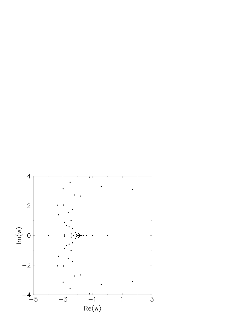
FIG. 2.: Potts zeros in the complex $w$ ($=Q^{1\over 2}$) plane of the partition function $Z_{CP}$ for the $8\times 8$ square lattice with self-dual boundary conditions.

FIG. 3.: Potts zeros in the complex $Q$ plane of the critical Potts model for the $8\times 8$ square lattice with free boundary conditions.

FIG. 4.: Fisher zeros in the complex $p$ plane of the $Q$-state Potts model on the $4\times 4$ square lattice with self-dual boundary conditions for (a) $Q=75$ and (b) $Q=76$.

FIG. 5.: Potts zeros in the complex $Q$ plane of the chromatic polynomial on the $8\times 8$ square lattice for cylindrical [15] and self-dual boundary conditions.

FIG. 6.: Potts zeros of the dichromatic polynomial for $0\leq a\leq 1$ on the $7\times 7$ square lattice with self-dual boundary conditions.

FIG. 7.: BST extrapolation of $Q_{c}^{AF}$ as a function of $a$ for self-dual boundary conditions. The continuous curve is given by $Q_{c}=(1-a)(a+3)$.

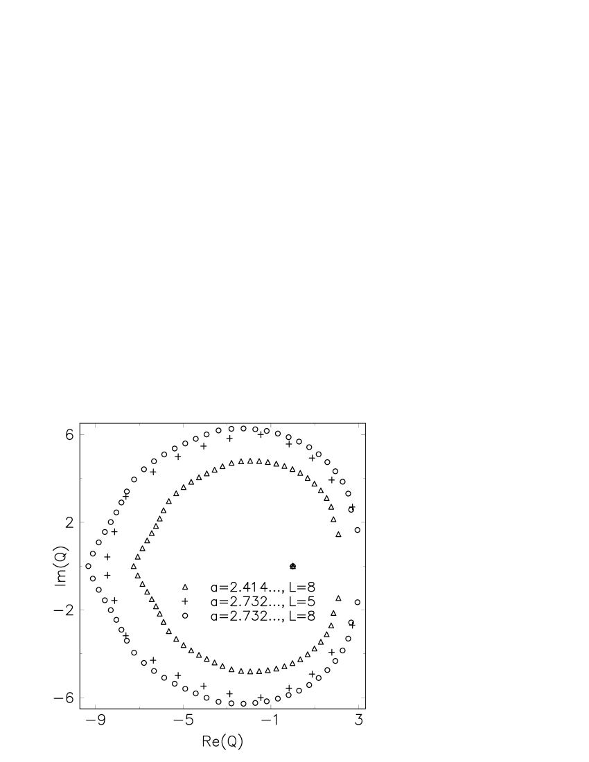
FIG. 8.: Potts zeros in the complex $Q$ plane of the dichromatic polynomial on the $L\times L$ square lattices with cylindrical boundary conditions for $a>1$.

FIG. 9.: BST extrapolation of $Q_{c}^{FM}$ as a function of $a$ for self-dual boundary conditions. The continuous curve is given by $Q_{c}=(a-1)^{2}$.

FIG. 10.: The exponent $y_{q}$ as a function of $a$ for free, cylindrical, and self-dual boundary conditions. The slight horizontal offset for data for cylindrical and self-dual boundary conditions is for clarity only. The long-dashed curve is the thermal exponent $y_{t}$ by the den Nijs formula.

FIG. 11.: Fisher zeros in the complex $p$ plane of the three-state Potts model on $12\times 12$ square lattice with free boundary conditions. The dotted line is the antiferromagnetic interval.

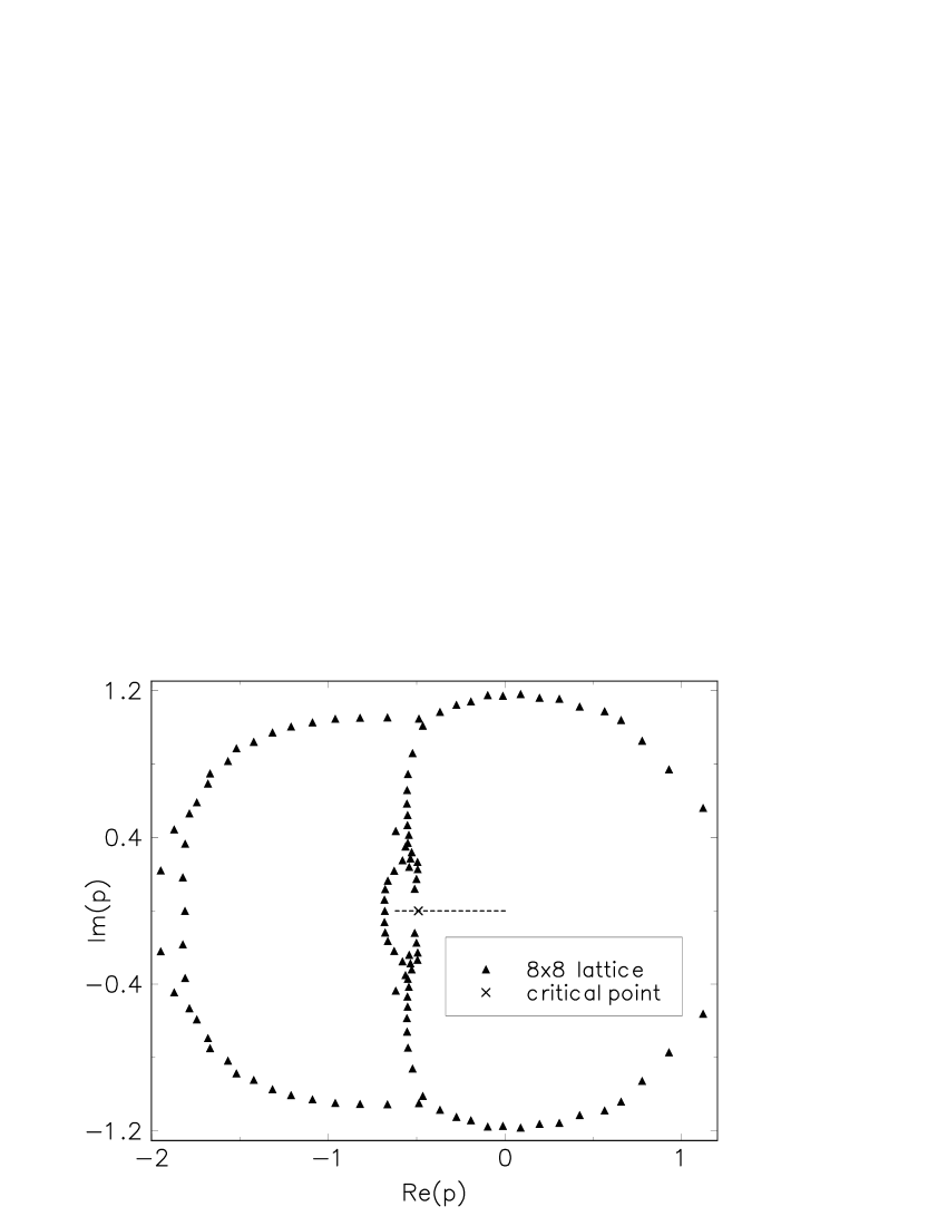
FIG. 12.: Fisher zeros in the complex $p$ plane of the $Q=2.5$ Potts model on $8\times 8$ square lattice with free boundary conditions. The dotted line shows the antiferromagnetic interval.

FIG. 13.: The thermal exponents $y_{t}$ of the $Q$-state Potts antiferromagnets by the BST estimates (filled circles) from data for $L=3\sim 8$ and free boundary conditions. For $Q=3$ the BST estimate (filled triangle) from data for $L=3\sim 12$ is added and has the slight horizontal offset for clarity only.

FIG. 14.: BST extrapolation of the imaginary part of the critical point, ${\rm Im}(a_{c})$, for the three-state Potts antiferromagnet as a function of the parameter $\omega$.

REFERENCES

- [1] F. Y. Wu, Rev. Mod. Phys. 54, 235 (1982), and references therein.
- [2] R. J. Baxter, J. Phys. C 6, L445 (1973).
- [3] M. P. M. den Nijs, J. Phys. A 12, 1857 (1979); B. Nienhuis, E. K. Riedel, and M. Schick, J. Phys. A 13, L31 (1980); J. L. Black and V. J. Emery, Phys. Rev. B 23, 429 (1981); B. Nienhuis, J. Phys. A 15, 199 (1982).
- [4] R. B. Pearson, Phys. Rev. B 22, 2579 (1980); B. Nienhuis, E. K. Riedel, and M. Schick, J. Phys. A 13, L189 (1980); M. P. M. den Nijs, Phys. Rev. B 27, 1674 (1983).
- [5] H. W. J. Blöte, M. P. Nightingale, and B. Derrida, J. Phys. A 14, L45 (1981); H. W. J. Blöte and M. P. Nightingale, Physica A 112, 405 (1982).
- [6] G. S. Grest and J. R. Banavar, Phys. Rev. Lett. 46, 1458 (1981).
- [7] J. L. Cardy, Phys. Rev. B 24, 5128 (1981).
- [8] C. Jayaprakash and J. Tobochnik, Phys. Rev. B 25, 4890 (1982).
- [9] M. P. Nightingale and M. Schick, J. Phys. A 15, L39 (1982).
- [10] R. J. Baxter, Proc. R. Soc. London A 383, 43 (1982).
- [11] M. P. M. den Nijs, M. P. Nightingale, and M. Schick, Phys. Rev. B 26, 2490 (1982).
- [12] T. Temesvári, J. Phys. A 15, L625 (1982).
- [13] F. Fucito, J. Phys. A 16, L541 (1983).
- [14] Z. Rácz and T. Vicsek, Phys. Rev. B 27, 2992 (1983).
- [15] J. Kolafa, J. Phys. A 17, L777 (1984).
- [16] J.-S. Wang, R. H. Swendsen, and R. Kotecký, Phys. Rev. Lett. 63, 109 (1989); Phys. Rev. B 42, 2465 (1990).
- [17] H. Park and M. Widom, Phys. Rev. Lett. 63, 1193 (1989).
- [18] H. Saleur, Nucl. Phys. B 360, 219 (1991).
- [19] A. Bakchich, A. Benyoussef, and M. Touzani, Physica A 192, 516 (1993).
- [20] S. J. Ferreira and A. D. Sokal, Phys. Rev. B 51, 6727 (1995).
- [21] J. K. Burton Jr. and C. L. Henley, J. Phys. A 30, 8385 (1997).
- [22] J. Salas and A. D. Sokal, J. Stat. Phys. 92, 729 (1998).
- [23] R. Shrock and S.-H. Tsai, Phys. Rev. E 58, 4332 (1998).
- [24] S. J. Ferreira and A. D. Sokal, J. Stat. Phys. 96, 461 (1999).
- [25] C. Moore, M. G. Nordahl, N. Minar, and C. R. Shalizi, Phys. Rev. E 60, 5344 (1999).
- [26] R. Shrock, Physica A 281, 221 (2000).
- [27] S.-Y. Kim, R. J. Creswick, C.-N. Chen, and C.-K. Hu, Physica A 281, 262 (2000).
- [28] C. N. Yang and T. D. Lee, Phys. Rev. 87, 404 (1952); T. D. Lee and C. N. Yang, ibid. 87, 410 (1952).
- [29] R. J. Creswick and S.-Y. Kim, Phys. Rev. E 56, 2418 (1997); Comput. Phys. Commun. 121, 26 (1999), and references therein.
- [30] R. Kenna and A. C. Irving, Nucl. Phys. B 485, 583 (1997), and references therein.
- [31] S.-Y. Kim and R. J. Creswick, Phys. Rev. Lett. 81, 2000 (1998); Physica A 281, 252 (2000).
- [32] M. E. Fisher, in Lectures in Theoretical Physics, edited by W. E. Brittin (University of Colorado Press, Boulder, 1965), Vol. 7c, p. 1.
- [33] J. M. Maillard and R. Rammal, J. Phys. A 16, 353 (1983).
- [34] P. P. Martin, Nucl. Phys. B 225, 497 (1983).
- [35] P. P. Martin, in Integrable Systems in Statistical Mechanics, edited by G. M. D’Ariano, A. Montorsi, and M. G. Rasetti (World Scientific, Singapore, 1985), p. 129.
- [36] P. P. Martin, J. Phys. A 19, 3267 (1986).
- [37] D. W. Wood, R. W. Turnbull, and J. K. Ball, J. Phys. A 20, 3465 (1987).
- [38] G. Bhanot, J. Stat. Phys. 60, 55 (1990).
- [39] N. A. Alves, B. A. Berg, and R. Villanova, Phys. Rev. B 43, 5846 (1991).
- [40] P. P. Martin, Potts Models and Related Problems in Statistical Mechanics (World Scientific, Singapore, 1991).
- [41] C.-N. Chen, C.-K. Hu, and F. Y. Wu, Phys. Rev. Lett. 76, 169 (1996).
- [42] F. Y. Wu, G. Rollet, H. Y. Huang, J. M. Maillard, C.-K. Hu, and C.-N. Chen, Phys. Rev. Lett. 76, 173 (1996).
- [43] V. Matveev and R. Shrock, Phys. Rev. E 54, 6174 (1996).
- [44] R. J. Creswick and S.-Y. Kim, in Computer Simulation Studies in Condensed-Matter Physics, edited by D. P. Landau, K. K. Mon, and H.-B. Schüttler (Springer, Berlin, 1998), Vol. 10, p. 224. [cond-mat/9909390]
- [45] R. Kenna, J. Phys. A 31, 9419 (1998); Nucl. Phys. B, Proc. Suppl. 63, 646 (1998).
- [46] S.-Y. Kim and R. J. Creswick, Phys. Rev. E 58, 7006 (1998).
- [47] R. J. Baxter, J. Phys. A 20, 5241 (1987), and references therein.
- [48] R. Shrock and S.-H. Tsai, Phys. Rev. E 55, 5165 (1997).
- [49] N. Biggs and R. Shrock, J. Phys. A 32, L489 (1999).
- [50] R. Shrock, cond-mat/9908387 (in Proceedings of the 1999 British Combinatorial Conference), Chromatic polynomials and their zeros and asymptotic limits for families of graphs, and references therein.
- [51] A. D. Sokal, cond-mat/9904146 (Combin. Prob. Comput., in press), Bounds on the complex zeros of (di)chromatic polynomials and Potts-model partition functions, and references therein.
- [52] R. J. Creswick, Phys. Rev. E 52, 5735 (1995).
- [53] P. W. Kasteleyn and C. M. Fortuin, J. Phys. Soc. Jpn. Suppl. 26, 11 (1969); C. M. Fortuin and P. W. Kasteleyn, Physica 57, 536 (1972).
- [54] C.-N. Chen and C.-K. Hu, Phys. Rev. B 43, 11519 (1991).
- [55] J. Hoshen and R. Kopelman, Phys. Rev. B 14, 3438 (1976).
- [56] R. Bulirsch and J. Stoer, Numer. Math. 6, 413 (1964); M. Henkel and G. Schütz, J. Phys. A 21, 2617 (1988).
- [57] C. Itzykson, R. B. Pearson, and J. B. Zuber, Nucl. Phys. B 220, 415 (1983).
- [58] M. L. Glasser, V. Privman, and L. S. Schulman, Phys. Rev. B 35, 1841 (1987).
- [59] K.-C. Lee, J. Phys. A 28, 4835 (1995); C. M. Care, ibid. 29, L505 (1996), and references therein.