Instanton picture of the spin tunneling in the Lipkin model

Abstract

A consistent theory of the ground state energy and its splitting due to the process of tunneling for the Lipkin model is presented. For the functional integral in terms of the spin coherent states for the partition function of the model we accurately calculate the trivial and the instanton saddle point contributions. We show that such calculation has to be perfomed very accurately taking into account the discrete nature of the functional integral. Such accurate consideration leads to finite corrections to a naive continous consideration. We present comparison with numerical calculation of the ground state energy and the tunneling splitting and with the results obtained by the quasiclassical method and get excellent agreement.

I Introduction

Lipkin, Meshkov and Glick [1] proposed in 1965 an exactly solvable two-level many-fermion model which has been used to test various kinds of many-body theories. The model Hamiltonian reads

$$H=\tilde{\omega}\hat{S}_{0}-\frac{1}{2}f(\hat{S}_{+}^{2}+\hat{S}_{-}^{2})$$ (1)

where $f$ is the coupling constant, $\tilde{\omega}$ is the energy difference between the two levels,

$$\hat{S}_{0}=\frac{1}{2}\sum_{m=1}^{\Omega}(c_{+m}^{{\dagger}}c_{+m}-c_{-m}^{{\dagger}}c_{-m}),$$ (2)

$$\hat{S}_{+}={1\over 2}\sum_{m=1}^{\Omega}c_{+m}^{{\dagger}}c_{-m},\quad\hat{S}_{-}=\hat{S}_{+}^{{\dagger}},$$ (3)

and $\Omega$ is the degree of degeneracy of each level. The single particle states are labeled by the quantum numbers $\pm m.$ The operators $\hat{S}_{0},\hat{S}_{\pm}$ satisfy the commutation relations of the $su(2)$ algebra.

The transformation associated with the unitary operator ${\rm e}^{i\pi\hat{S}_{0}}$ leaves the Hamiltonian invariant. If $\chi=f\Omega/\tilde{\omega}<1,$ the mean field groundstate of the model is classified according to the trivial representation of the symmetry group. The symmetry is spontaneously broken if $\chi>1.$

A splitting of the levels is then observed, which is analogous to the occurrence of rotational bands in deformed nuclei. The model is also of great interest in condensed matter physics, since it is related to the anysotropic Heisenberg model. In the strong coupling limit, $\chi\gg 1,$ the level splitting vanishes for odd $\Omega.$ This behaviour is easily understood in the framework of Kramers theorem and is related to the well known phenomenon of tunnelling suppression for odd spin anysotropic Heisenberg ferromagnets.

In this paper we formulate a general physical picture of the calculation of the ground state energy and its splitting by the instanton method. Such method was applied to the anisotropic Heisenberg model for description of the tunneling of the magnetic moment of small magnetic particles with large spin [2, 3, 4, 5, 6, 9]. Although the physical picture of the spin tunneling was formulated in these papers the quantitative results of the papers [3, 4, 5, 6, 9] are not completely correct.

We show that special care is required when computing the instanton contributions in order to take also correctly into account the small amplitude quantum fluctuations. On more technical language the functional determinants have to be calculated very accurately taking properly into account the operator ordering generating the functional integral for the partition sum. We show that it is essential to keep in mind that the fuctional integral is generated by the spin coherent state method. Taking accurately into account the discrete nature in time of the functional leads to essential corrections to the ground state energy and to its tunneling splitting. After taking into account all these contribution our result completely coinsides with the one of [2] obtained by the semiclassical method and the contradiction existing in literature is resolved.

The structure of the paper is as follws. In Sec. II we present the functional integral for the Lipkin model. In Sec. III we review the the simple results for the tunneling in the framework of the continuous approximation for the functional integral. In Sec. IV we calculated accurately the contribution of the trivial saddle point to the partition function and determine the ground state energy. In Sec. V we calculeted the determinant and the measure of integration over time in the framework of the canonical fromulation of the functional integral. In Sec. VI we calculate accurately the functional determinant for the instanton saddle point taking into account the corrections due to discretization. In Sec. VII we present comparison between the analytical theory and the numerical calculations for the Lipkin model and find an excellent agreement when additional contributions discovered in this paper are taken into account.

II Functional integral for the Lipkin model

It is convenient to rewrite the Hamiltonian of the model in the rotated reference frame

$$\hat{H}=\hat{H}_{2}+\hat{H}_{1},\ \ \ \hat{H}_{1}=\tilde{\omega}\hat{S}_{y},$$ (4)

$$\hat{H}_{2}=f(\hat{S}_{z}^{2}-\hat{S}_{x}^{2})=f\biggl{(}{3\over 2}\hat{S}_{z}^{2}-{1\over 2}s(s+1)-{1\over 4}(\hat{S}_{+}^{2}+\hat{S}_{-}^{2})\biggr{)}.$$ (5)

Here we assume that the magnitude of spin $s\gg 1$. The first term in the Hamiltonian (4) describes interaction between nucleons, the second one represents an energy splitting and can be regarded as an external magnetic field. The choice of the coordinate axis is determined by the convenience condition for further calculations.

The Lipkin model can be reduced to the anisotropic Heisenberg model [3]. For that we add to the Hamiltonian (4) the term $f(S_{x}^{2}+S_{y}^{2}+S_{z}^{2}-s(s+1))=0$ and the Hamiltonian (4) takes the form

$$\hat{H}=-fs(s+1)+f(2\hat{S}_{z}^{2}+\hat{S}_{y}^{2})+\tilde{\omega}S_{y}.$$ (6)

In the language of the Heisenberg model the magnetic field here is in the direction of the second axis $y$. The parameter $\lambda$ of the paper [3] is $1/2$ for our case. We concentrate our attention on the accurate treatment of the ground state energy of the model and its tunneling splitting when the second term in (4) is absent or $\tilde{\omega}=0$.

In this special case the Lipkin model is invariant under the time reflection. In the case of half-integer spin $s$ this symmetry leads to the two-fold Kramer’s degeneracy of the ground state [5, 6]. In the case of integer spin $s$ instead of degeneracy we have the splitting of the ground state. This splitting has to be small because for large $s$ the difference between integer and half-integer spin has to be small. In fact this splitting is exponentially small.

To solve this problem we have used the instanton method [7] applied to the functional integral for the partition function of our spin system in terms of spin coherent states [8]. The coherent states are given by the following formula [8]:

$$|z\rangle=(1+|z|^{2})^{-s}\exp(z\hat{S}_{+})|0\rangle,\ \ \ \hat{S}_{-}|0\rangle=0,$$ (7)

$$\hat{S}_{z}|0\rangle=-s|0\rangle,$$ (8)

where $z$ is a complex number. They possess many remarkable properties and with the help of them the partition function can be represented in the form [8]:

$$Z=Tr[\exp(-T\hat{H})],$$ (9)

$$Z=\int_{-\infty}^{\infty}\cdot\cdot\cdot\int_{-\infty}^{\infty}\prod_{n=0}^{N-1}\frac{(2s+1)dz_{n}dz^{*}_{n}}{\pi(1+|z_{n}|^{2})^{2}}\exp(A(z)).$$ (10)

Here the interval of the imaginary time $T$ is split into $N$ parts: $T=N\Delta$, and in every section an integration over $z^{\prime}_{n}=\mbox{Re}z_{n}$ and $z^{\prime\prime}_{n}=\mbox{Im}z_{n}$ is performed. The action of the system $A(z)$ has the form

$$A(z)=\sum_{n=0}^{N-1}[2s\ln(1+z^{*}_{n+1}z_{n})-$$ (11)

$$2s\ln(1+|z_{n}|^{2})-\Delta H(z^{*}_{n+1},z_{n})],$$ (12)

where the variables $z_{n}$ satisfy the periodic boundary conditions: $z_{N}=z_{0}$ or in the continuum limit $z(T)=z(0)$, and the Hamiltonian

$$H(z^{*}_{n+1},z_{n})=\frac{\langle z_{n+1}|\hat{H}|z_{n}\rangle}{\langle z_{n+1}|z_{n}\rangle}.$$ (13)

The matrix elements of all essential operators have the form

$$\langle z|\hat{S}_{0}|z^{\prime}\rangle=-s(1-z^{*}z^{\prime})(1+z^{*}z^{\prime})Q_{s},\ \$$ (14)

$$\langle z|\hat{S}_{-}|z^{\prime}\rangle=2sz^{\prime}(1+z^{*}z^{\prime})Q_{s},$$ (15)

$$\langle z|\hat{S}_{+}|z^{\prime}\rangle=2sz^{*}(1+z^{*}z^{\prime})Q_{s},\ \$$ (16)

$$\langle z|\hat{S}^{2}_{+}|z^{\prime}\rangle=2s(2s-1)z^{*2}Q_{s},$$ (17)

$$\langle z|\hat{S}^{2}_{-}|z^{\prime}\rangle=2s(2s-1)z^{\prime 2}Q_{s},\ \$$ (18)

$$\langle z|\hat{S}^{2}_{0}|z^{\prime}\rangle=(s^{2}(1+z^{*}z^{\prime})^{2}-2s(2s-1)z^{*}z^{\prime})Q_{s}$$ (19)

$$\langle z|z^{\prime}\rangle=(1+z^{*}z^{\prime})^{2}Q_{s},\ \$$ (20)

$$Q_{s}=(1+z^{*}z^{\prime})^{2s-2}/(1+|z|^{2})^{s}(1+|z^{\prime}|^{2})^{s}.$$ (21)

III Naive classical picture for the ground state energy and its instanton splitting

A Classical action and its minima

In many cases (but not in all !) one can take the continuum limit when $z_{n+1}$ is close to $z_{n}$. In this continuum limit it is convenient to introduce the canonically conjugated variables $\varphi$ and $p=\cos\theta$:

$$z=\rho\exp{(i\varphi)},\ \ \ \rho^{2}=\frac{s-p}{s+p},\ \ \ \begin{array}[]{c}0\leq\varphi\leq 2\pi,\\ -s\leq p\leq s\end{array}.$$ (24)

The action of the system $A(z)$ in the continuum limit is

$$A(\varphi,p)=\int_{0}^{T}[i(p-s)\dot{\varphi}-H(p,\varphi)]dt,$$ (25)

$$H(p,\varphi)=(g/2)(p^{2}(1+\cos^{2}\varphi)-s^{2}\cos^{2}\varphi),$$ (26)

where $H(p,\varphi)$ is the Hamiltonian of the problem, $g=f(2S-1)/S,\ \ g>0$ is the coupling constant. This Hamiltonian is unusual because the mass depends on the coordinate $\varphi$. The second essential peculiarity is the presence in the action of the term $is\dot{\varphi}$ which separates integer and half-integer spins [5, 6]. In spite of that the ground state energy and the splitting can be found.

One can easily check that the Hamiltonian has two minima at the points $\varphi=0,\ \pi$ and $p=0$. These minima are deep for $s\gg 1$ and the Hamiltonian in the neighborhood of the minima has the simple form of a harmonic oscillator

$$H(p,\varphi)=E_{min}+gp^{2}+gs^{2}\varphi^{2}/2,\ \ \ E_{min}=-s^{2}g/2$$ (27)

and the vibration frequency is $\omega=\sqrt{2}gs$. One can assume that the energy of the ground state

$$E_{0\ naive}=E_{min}+\hbar\omega/2.$$ (28)

This expression for $E_{0}$ can be obtained if we calculate the contribution of the trivial saddle piont to the partition function by the method of [7].

B The instanton contribution to the splitting of the ground state

Besides the trivial saddle point contribution to the partition function discussed above (11) there exists a set of nontrivial saddle point contributions. These saddle points, in their main features, can be discussed in terms of the continuum action (25). The discussion of the Gaussian fluctuations around the saddle points has to be done more accurately but the result can be expressed in terms of the continuum action only. The instanton saddle points for the action (25) are realized at the imaginary momentum $p_{t}=isu_{t}$. The Hamiltonian equations of motion which follow from (25) are:

$$\dot{\varphi}=gs(1+\cos^{2}\varphi)u,$$ (29)

$$\dot{u}=gs\sin\varphi\cos\varphi(1+u^{2}).$$ (30)

We are interested in the time periodic solution of Eqs. (29): $\varphi(0)=\varphi(T),\ p(0)=p(T)$. These periodic solutions can be constructed from the elementary solutions which are named instantons and anti–instantons. It is obvious from Fig. 1 that there are two types of instantons (A and B) and two types of anti–instantons ($\bar{A}$ and $\bar{B}$) for our problem.

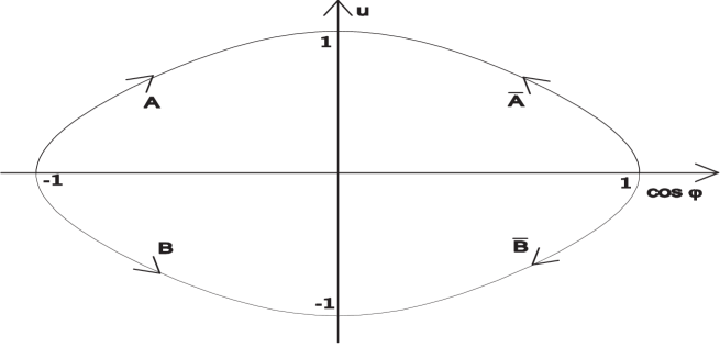
FIG. 1.: Instanton trajectories in the phase $cos(\varphi)-u$ space. The curve A corresponds to the $A$–instanton and $\bar{A}$ antiinstanton, the curve B corresponds to the B-instanton and $\bar{B}$ antiinstanton. $cos(\varphi)$ is along the horizontal axis, the momentum $u$ is along the vertical axis.

Each of them is labeled by the time $t_{0}$ at which $\cos(\varphi(t_{0}))=0$ and $u(t_{0})=\pm 1$.

The A–instanton starts at the time $t\rightarrow-\infty$ from the point of phase space $(\varphi=-\pi,u=0)$ at the time $t=t_{0}$ arrives at the point $(\varphi=0,u=-1)$ and at the time $t\rightarrow\infty$ arrives at the point $(\varphi=\pi,u=0)$.

The B–instanton starts at the time $t\rightarrow-\infty$ from the point of phase space $(\varphi=-\pi,u=0)$ at the time $t=t_{0}$ arrives at the point $(\varphi=0,u=1)$ and at the time $t\rightarrow\infty$ arrives at the point $(\varphi=\pi,u=0)$.

The A–anti–instanton starts at the time $t\rightarrow-\infty$ from the point of phase space $(\varphi=\pi,u=0)$ at the time $t=t_{0}$ arrives at the point $(\varphi=0,u=1)$ and at the time $t\rightarrow\infty$ arrives at the point $(\varphi=-\pi,u=0)$.

The B–anti–instanton starts at the time $t\rightarrow-\infty$ from the point of phase space $(\varphi=\pi,u=0)$ at the time $t=t_{0}$ arrives at the point $(\varphi=0,u=1)$ and at the time $t\rightarrow\infty$ arrives at the point $(\varphi=-\pi,u=0)$.

The analytic form of these solutions can be easily constructed if we take into account the energy conservation during the process of motion $H(u,\varphi)=E_{min}$. In this case we have the following algebraic connection between $p$ and $\varphi$:

$$u^{2}=\frac{1-\cos^{2}\varphi}{1+\cos^{2}\varphi}.$$ (31)

Combining formula (29) and (31) we get the equation of motion for instantons and anti–instantons:

$$\dot{\varphi}=\pm gs\sqrt{1-\cos^{4}\varphi},$$ (32)

where the sign $\pm$ corresponds to the two types of instantons. This equation of motion can be easily solved and we have

$$\cos\varphi_{t}^{0}=\pm\frac{\sinh(\tau_{0})}{\sqrt{2+\sinh^{2}(\tau_{0})}},\ \ \ u_{t}^{0}=\mp\frac{1}{\cosh(\tau_{0})},$$ (33)

where $\tau_{0}=\omega(t-t_{0})$.

The instanton action $A_{0}$ counting from the energy minimum is

$$A_{0}=gs^{2}\int_{0}^{T}(1-\cos^{2}\varphi)dt=$$ (34)

$$s\int_{0}^{\pi}\sqrt{(1-\cos^{2}\varphi)\over(1+\cos^{2}\varphi)}d\varphi=2s\ln(1+\sqrt{2}).$$ (35)

The calculation of the instantons and anti–instantons contribution to the partition function is based on the idea of an approximate saddle point. The general trajectory for an approximate saddle point is shown in Fig. 2.

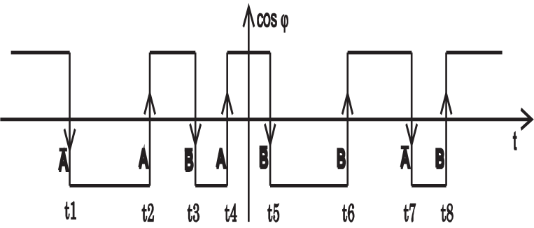
FIG. 2.: The scheme of the consecutive fast instanton and antiinstanton transitions at times $t_{1},\ t_{2},...\ t_{8}$. The time $t$ is along the horizontal axis, $\cos(\varphi)$ is along the vertical axis.

This trajectory starts from the point $\varphi=\pi,\ u=0$ and finishes at the same one. It represents a sequence of fast instanton and anti–instanton transitions (A and B types). The centers of theses instantons and anti–instantons (points where $\varphi=\pm\pi/2,\ u=\pm 1$) are situated at the arbitrary (but ordered points) $t_{l}$. Notice, that for the exact solution we have a periodical lattice of instantons and anti–instantons. The contribution of an approximate saddle point to the partition function can be presented in the form ([7]):

$$Z_{apr}^{n}=\int_{0}^{T}\cdot\cdot\cdot\int_{0}^{T}\prod_{l=1}^{n-1}\theta(t_{l+1}-t_{l})\cdot$$ (36)

$$\prod_{l=1}^{n}[Ke^{-A_{0}-is\varphi_{l}}dt_{l}][{\det}^{\prime}(\hat{L}_{sad})]^{-1/2}.$$ (37)

The integral over the positions of the instantons $t_{l}$ in Eq. (36) represents a sum of contributions to the partition function over the manifold with almost the same action $A_{0}$. The factor $K^{n}$ gives the measure of the integration over degenerate minima [7]. Its explicit form can be derived if we connect the time $t_{l}$ with the amplitude of the zero mode of the quadratic form $\hat{L}_{ins}$ describing of the fluctuations around of the instanton solution. The factor $\exp(-A_{0}-is\varphi_{l})$ gives the exponent contribution to the partition function. The quantity $s\varphi_{l}$ is the Berry phase which follows from Eq. (25) for the continuum action. This phase $s\varphi_{l}$ is equal to $s\pi$ for $A$–instanton and $\bar{B}$–anti–instanton and $-s\pi$ for $B$–instanton and $\bar{A}$–anti–instanton.

The last factor in Eq. (36), ${\det}^{\prime}(\hat{L}_{sad})$, represents the determinant of the quadratic form describing fluctuations around the approximate saddle point solution excluding eigenvalues corresponding to zero mode fluctuations. We understand the determinant as a product of the eigenvalues of the corresponding quadratic form. Our aim is to describe the calculation of this determinant in more detail.

(1). One can represent ${\det}^{\prime}(\hat{L}_{sad})$ as a product

$${\det}^{\prime}(\hat{L}_{sad})=\det(\hat{L}_{0})\cdot X,\ \ \ X={\det}^{\prime}(\hat{L}_{sad})/\det(\hat{L}_{0}),$$ (38)

where $\det(\hat{L}_{0})$ is the determinant of the trivial saddle point which we calculate in Sec. VI (66). It is important to notice that the magnitudes of determinants ${\det}^{\prime}(\hat{L}_{sad})$ and $\det(\hat{L}_{0})$ depend on the method of regularization of the functional integral for the partition function or (what is just the same) from the large eigenvalues of the quadratic forms $\hat{L}_{sad}$ and $\hat{L}_{0}$. But it is obvious (see Fig. 3) that for $T\omega/n\gg 1$ the large eigenvalues of the quadratic forms $\hat{L}_{sad}$ and $\hat{L}_{0}$ are the same because during almost all time of motion the variables $\varphi(t)$ and $u(t)$ are close to the trivial saddle points where $\varphi=0,\ \pi$ and $u=0$.

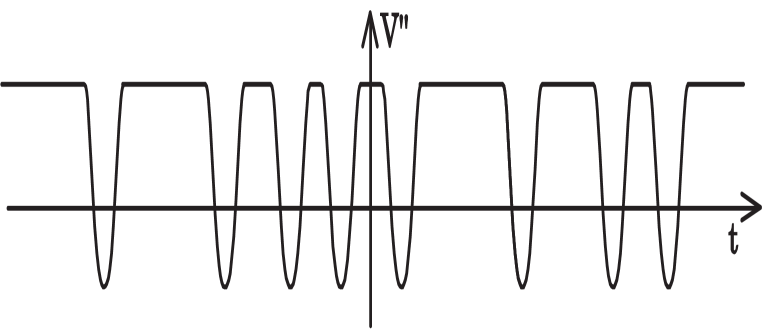
FIG. 3.: The effective potential energy for the ”particle” in the field of many instanton transitions. The time $t$ is along the horizontal axis the effective potential energy is along the vertical axis.

This means that the quadratic forms $\hat{L}_{sad}$ and $\hat{L}_{0}$ differ from each other only during the time $n/\omega\ll T$. This means that the quantity $X$ can be presented as the ratio of determinants in the continuum limit

$$X={\det}^{\prime}(\hat{L}_{sad\ cont})/\det(\hat{L}_{0\ cont}).$$ (39)

(2). For simplification of the problem it is convenient to integrate the action over the variable $p$. For that we spread the limits of integration to $\pm\infty$ in the expression (25) for the partition function. Such spreading of the limits of integration can be justified in the case

$$g\Delta s^{2}\gg 1,\ \ \mbox{or}\ \ s\gg 1/\Delta\omega,\ \ \ \Delta\omega\ll 1.$$ (40)

Because $\Delta\omega<0.1$ this leads to conclusion that such integration is justified for $s\gg 10$. We want to stress that this condition includes the time quantization step $\Delta$. Therefore the expression for the partition function takes the form of a functional integral over the variable $\varphi$, and in the leading approximation over $1/s$ we have

$$Z=\int_{0}^{2\pi}\cdot\cdot\cdot\int_{0}^{2\pi}e^{A_{B}+A_{\varphi}}\prod_{t=0}^{T}\frac{d\varphi_{t}}{\sqrt{2\pi\Delta g(1+\cos^{2}\varphi_{t})}},$$ (41)

$$A_{B}=-is\int_{0}^{T}\dot{\varphi}_{t}\ dt,\ \ \$$ (42)

$$A_{\varphi}=-(1/2)\int_{0}^{T}\biggl{(}\dot{\varphi}^{2}_{t}/g(1+\cos^{2}\varphi_{t})-gs^{2}\cos^{2}\varphi_{t}\biggr{)}dt,$$ (43)

where $A_{B}$ is the Berry phase, $A_{\varphi}$ is the action of the field $\varphi$. We want to remind that the measure of integration of the functional integral over configuration space depends on the time step $\Delta$.

It is natural to introduce a new variable $\psi_{t}$ in the functional integral (41) through relations:

$$d\psi_{t}=(g(1+\cos^{2}\varphi_{t}))^{-1/2}d\varphi_{t},$$ (44)

$$\psi_{t}=\int_{0}^{\varphi_{t}}(g(1+\cos^{2}y))^{-1/2}dy.$$ (45)

The explicit form of $\psi_{t}$ as function of $\varphi_{t}$ is an elliptic function but this explicit form is unnecessary for further calculations. In terms of $\psi_{t}$ the action $A_{\varphi}$ takes the canonical form

$$A_{\varphi}=-(1/2)\int_{0}^{T}[\dot{\psi}_{t}^{2}-gs^{2}\cos^{2}\varphi_{t}]\ dt,$$ (46)

where $\varphi_{t}$ in this formula is a function of $\psi_{t}$. One can check that this action has the instantons minima for $\cos\varphi^{0}_{t}$ according to Eq. (33) and the instanton action $A_{0}$ according to (34). Decomposing the action (46) around the multi-instanton minima and using (44) we get the part of the action quadratic in fluctuations in the form

$$A_{\varphi}^{q}=-(1/2)\int[\delta\psi_{t}\ \hat{L}_{sad\ cont}\ \delta\psi_{t}]\ dt,$$ (47)

$$\hat{L}_{sad\ cont}=-\frac{\partial^{2}}{\partial t^{2}}+V^{\prime\prime}(\varphi_{t}^{0}),\ \ \$$ (48)

$$V^{\prime\prime}(\varphi_{t}^{0})=\frac{\omega^{2}}{2}(2\cos^{2}\varphi_{t}^{0}-1)(1+\cos^{2}\varphi_{t}^{0}).$$ (49)

The function $V^{\prime\prime}(\varphi_{t}^{0})$ plays the role of the potential energy for the problem of fluctuations around the instantons (see Fig.3). For the trivial saddle point $\cos^{2}\varphi_{t}=1$, $V^{\prime\prime}(\varphi_{t}^{0})=\omega^{2}$ and the operator $\hat{L}_{0\ cont}$ has the simple form:

$$\hat{L}_{0\ cont}=-\frac{\partial^{2}}{\partial t^{2}}+\omega^{2}.$$ (50)

The typical function $V^{\prime\prime}(\varphi_{t}^{0})$ is shown in Fig. 3. It is equal to $\omega^{2}$ in almost all region $0\leq t\leq T$, excluding narrow regions of order $1/\omega$ around the instanton transitions at points $t=t_{l}$ where it has wells of depth $-\omega^{2}/2$.

(3). At this point we can calculate the ratio of determinants $X$ (39). This calculation is based on the small parameter $n/\omega T\ll 1$ and we can prove that the ratio $X$ is equal to the product of the ratio of determinants for each region containing an instanton or an anti–instanton:

$$X=\prod_{l=1}^{n}X_{l},\ \ \ X_{l}={\det}^{\prime}(\hat{L}_{l,\ ins\ cont})/\det(\hat{L}_{l,\ 0\ cont}),$$ (51)

where the operators $\hat{L}_{l,\ ins\ cont}$ and $\hat{L}_{l,\ 0\ cont}$ are defined in the region $((t_{l+1}+t_{l})/2,\ (t_{l}+t_{l-1})/2)$ around the position $l$–instanton $t_{l}$ on the class of functions which satisfy the zero boundary conditions at the points $((t_{l+1}+t_{l})/2$ and $(t_{l}+t_{l-1})/2)$. This statement can be justified by the following arguments. Every determinant $\det(\hat{d})$ is the product of the eigenvalues of the operator $\hat{d}$ on some class of functions. In our case we can consider the class of functions with zero boundary conditions at points $((t_{l+1}+t_{l})/2$ and $(t_{l}+t_{l-1})/2)$. In this case all eigenvalues will be nondegenerated. For example, for the periodic boundary conditions they will be twice degenerated what is inconvenient. All eigenfunctions of the operator $\hat{d}$ in the region $[0,\ T]$ can be divided into two classes: those localized close to the instanton positions $t_{l}$ with the ”bounded” eigenvalues forming almost degenerated groups of $n$ eigenvalues and the propagating eigenfunctions with ”continuum” eigenvalues almost the same as in the case of the trivial saddle point. It is obvious that the contribution of the ”bounded” eigenvalues to the total determinant can be presented as the product of $n$ contributions. The ”continuum” eigenvalues can be calculated in the quasiclassical approximation and can also be split into $n$ parts. This argument proves the validity of Eq. (51).

(4). Because our problem is reduced to the well-known one for the usual instantons we can use results of Coleman [7]. The quantities $X_{l}$ of Eq. (51) can be calculated if we construct the normalized eigenfunction $\chi(t)=N\dot{\psi}(t)$, with $N=1/\sqrt{A_{0}}$, of the operator $\hat{L}_{sad\ cont}$ (47) with zero eigenvalue [7]. The function $\chi(t)$ has a form

$$\chi(t)=-s\sqrt{2g/(A_{0}(2+\sinh^{2}\tau_{0}))},\ \ \ \tau_{0}=\omega(t-t_{0}),$$ (52)

with asymptotic behavior at $\tau_{0}\Rightarrow\infty$

$$\lim|\chi(t)|\Rightarrow A_{\tau}\exp(-|\tau_{0}|),\ \ A_{\tau}=2(2)^{1/4}\sqrt{s\omega/A_{0}}.$$ (53)

On the basis of this solution one can prove [7] that the quantity

$$X_{l}=1/(2A^{2}_{\tau})$$ (54)

and does not depends on $l$ and $t_{l}$. The final formula for ${\det}^{\prime}(\hat{L}_{sad})$ entering in Eq. (36) for the partition function $Z_{apr}^{n}$ can be easily obtained if we combine Eqs. (38,39,51)

$${\det}^{\prime}(\hat{L}_{sad})=\det(\hat{L}_{0})/(2A^{2}_{\tau})^{n}.$$ (55)

(5). The quantity $K$ from Eq. (36) for the partition function $Z_{apr}^{n}$, which gives the measure of integration over time [7], can be calculated if we take into account the explicit form of the measure $dG_{t}$ in the functional integral (41) for the partition function for $s\gg 1$

$$dG_{t}=d\psi_{t}/\sqrt{2\pi\Delta}\Rightarrow Kdt\ \ \mbox{with}\ \ K=\sqrt{A_{0}/2\pi}.$$ (56)

At present all quantities entering in Eq. (36) for $Z_{apr}^{n}$ are defined and we have

$$Z_{apr}^{n}=(\det(\hat{L}_{0}))^{-1/2}(IT)^{n}\exp(-i\Phi)/n!,\ \$$ (57)

$$I=C\exp(-A_{0}),C=\sqrt{2\Delta}A_{\tau}K=2\ 2^{1/4}\omega\sqrt{s/\pi},$$ (58)

where $\Phi$ is the total Berry phase during all time of transitions.

For obtaning the final answer for $Z$ it is necessary to sum all saddle point contributions to the partition function. These total saddle point contributions can be presented in the form of the following sum:

$$Z=Z_{0}[1+(A+B)(\bar{A}+\bar{B})T^{2}/2+\ ...\$$ (59)

$$[(A+B)(\bar{A}+\bar{B})T^{2}]^{n}/(2n!)+\ ...].$$ (60)

where $Z_{0}$ is the contribution of the trivial saddle point, $A,B,\bar{A},\bar{B}$ are instanton and anti–instanton without the determinant of the trivial saddle point. The dependence on the Berry phase can be easily determined:

$$A,\bar{B}=\exp(i\pi s)I,\ \ \ B,\bar{A}=\exp(-i\pi s)I,$$ (61)

$$(A+B)(\bar{A}+\bar{B})=4I^{2}\cos^{2}(\pi s).$$ (62)

After these calculations we can sum all terms of the expression (59) in the form of $\cosh(-T\Delta E/2)$ and write the final answer for the energy of the ground state and its splitting by taking into account the explicit form of $Z_{0}$ (80) for the trivial saddle point:

$$E_{\pm}=E_{0}\pm\delta E/2,\ \ \ E_{0}=E_{min}+\omega/2,$$ (63)

$$\delta E=8\ 2^{1/4}\omega\sqrt{s/\pi}\exp(-2s\ln(1+\sqrt{2}))\cos(\pi s)],$$ (64)

where $E_{min}=-gs^{2}/2,\ \omega=\sqrt{2}sg,\ g=f(2s-1)/s$.

We can see that this splitting is exponentially small for large $s$ and equals zero in the case of half–integer spins in full agreement with Kramers theorem [5, 6]. The cancellation of the splitting for the case of the half-integer spin takes place due to the compensation of the contributions of the instantons of $A$ and $B$ type to the partition function $Z$.

But, unfortunately, expressions (63) for the ground state energy $E_{0}$ and the instanton splitting $\delta E$ are valid only qualitatively. The correct answer for $E_{0}$ contains the correction $-3gs/4$ and for the instanton splitting $\delta E$ the additional factor $1/(1+\sqrt{2})$. The origin of these corrections is in the subtle nature of the functional integral which demands accurate treatments when we calculate functional determinants.

IV Energy of the ground state or the trivial saddle point contribution to the partition function

The expression $E_{0}$ for the ground state energy is wrong due to an incorrect definition of the product of operators at the same point in terms of the variables $\varphi$ and $p$. The natural variables for the functional integral (9) are the $z$–variables. The trivial saddle points in terms of these variables are $z=\pm 1$. In the neighborhood of the saddle points we can represent the $z$–variables in the form

$$z=\pm 1+\sqrt{2/s}\ a,\ \ \,z^{*}=\pm 1+\sqrt{2/s}\ a^{*}.$$ (65)

The quadratic part of the action close to the saddle point is

$$A_{q}(a)=\sum_{n=0}^{N-1}[(a^{*}_{n+1}a_{n}-a^{*}_{n}a_{n})-\alpha a^{*}_{n+1}a_{n}-$$ (66)

$$(\beta/2)(a^{*2}_{n+1}+a^{2}_{n})],$$ (67)

where $\alpha=3Tsg/N,\ \beta=Tsg/N$. The quadratic form $A_{q}(a)$ can be partly diagonalized if we pass to the $\omega$-representation for the variables $a_{n},\ a^{*}_{n}$:

$$a_{n}=N^{-1/2}\sum_{m=0}^{N-1}\exp(i\omega_{m}n)a_{m},$$ (68)

$$a^{*}_{n}=N^{-1/2}\sum_{m=0}^{N-1}\exp(-i\omega_{m}n)a^{*}_{m},$$ (69)

where $\omega_{m}=2\pi im/N$. The action in the $\omega$-representation has the form:

$$A_{q}(a)=\sum_{m=0}^{N-1}[((1-\alpha)\exp(-i\omega_{m})-1)a^{*}_{m}a_{m}-$$ (70)

$$\beta(a^{*}_{m}a^{*}_{N-m}+a_{m}a_{N-m})].$$ (71)

The Gaussian integrals with the quadratic form (68) can be easily performed and the determinant $D^{-1}$ can be obtained. The determinant $D$ is equal to the product of the eigenvalues $\lambda_{m}$ of the quadratic form (68)

$$\lambda_{m}=\alpha^{2}-\beta^{2}+2(1-\alpha)(1-\cos\omega_{m}),$$ (72)

The partition function $Z$ has the following expression in terms of $\lambda_{m}$:

$$Z=\exp(E_{min}T)Y,\ \ \ Y=\prod_{m=0}^{N-1}\lambda_{m}^{-1/2}.$$ (73)

For the calculation of the quantity $Y$ it is convenient to represent the eigenvalues $\lambda_{m}$ in the form

$$\lambda_{m}=\mu_{m}\mu_{N-m},\ \ \ \mu_{m}=b+c\exp(i\omega_{m}),$$ (74)

$$(b,c)=(1/2)\left(\sqrt{\alpha^{2}-\beta^{2}}\pm\sqrt{(2-\alpha)^{2}-\beta^{2}}\right)$$ (75)

$$\simeq\pm(1-\alpha/2\pm\sqrt{\alpha^{2}-\beta^{2}}/2).$$ (76)

In terms of the quantities $\mu_{m}$ we have for $Y$

$$Y=\prod_{m=0}^{N-1}\mu^{-1}_{m}=\exp[-\sum_{m=0}^{N-1}\ln(\mu_{m})]=$$ (77)

$$\exp[-N\ln(b)-\sum_{m=0}^{N-1}\ln(1+(c/b)\exp(i\omega_{m}))].$$ (78)

The sum over $m$ in Eq. (77) can be easily performed if we expand the logarithmic function in a series over $x=(c/b)\exp(i\omega_{m})$ and take into account only the terms $x^{p}$ with $p=kN$, where $k$ is integer, which give nonzero contributions. The result for $Y$ has the form

$$Y=b^{-N}(1-(c/b)^{N})^{-1}.$$ (79)

Using the property $\alpha,\ \beta,\ b,\ c\simeq 1+d/N$ we easily get for the partition function and the ground state energy

$$Z_{0}=2\exp[-E_{0}T][1-\exp(-\omega T)]^{-1},\ \ \$$ (80)

$$E_{0}=E_{min}+(\omega-\omega_{0})/2,$$ (81)

where $\omega=\sqrt{2}sg,\ \omega_{0}=3sg/2$. The factor $2$ in this formula takes into account the presence of two minima in the action or the two types of the low–frequency excitations.

We can see that the result (80) differs from the naive result $E_{0\ naive}$ obtained previously. From the point of view of the functional integral this difference is due to the contribution of the large eigenvalues of the quadratic form (66) which correspond to the large $\omega$ in the partition function (73). From the operator point of view the quadratic form (66) expressed in terms of operators (for example with the help of the Holstein – Primakoff representation with the quantization along $x$) has to be diagonalized with the help of the Bogoluibov’s $u-v$ transformation. As a result of such diagonalization the ground state energy is shifted by the amount $(\omega-\omega_{0})/2$.

V Calculation of the determinant and the measure of integration over time in the continuum approximation

A Calculation of the determinant

In this section we present the calculation of the ratio of the functional determinants (33) $X_{l}$ without the primary integration over the variable $p$ which permits us to avoid the artificial limitation (40) $g\Delta s^{2}\gg 1$. Our consideration is based on the arguments of Coleman [7] applied to the system of two differential equations of the first order in time. This system of equations can be easily obtained if we introduce the quantum corrections to the classical solution $\varphi_{t}^{0},\ u_{t}^{0}$ (33)

$$\psi_{t}=\sqrt{s}\delta\varphi_{t},\ \ \ \ v_{t}=\sqrt{s}\delta u_{t}.$$ (82)

The quantum correction to the action has the form

$$A_{2}=-(1/2)\int_{-T/2}^{T/2}y_{ti}\hat{L}^{ij}_{0\ cont}y_{tj}dt,\ \ \ i,j=1,2,$$ (83)

where $y_{t1}=\psi_{t},\ y_{t2}=v_{t}$ and the $2\times 2$ matrix $\hat{L}_{0}$ can be presented in the form

$$\hat{L}_{0}=-\hat{\epsilon}\frac{\partial}{\partial t}+\hat{B},\ \ \ \hat{\epsilon}^{2}=-1,$$ (84)

$$\hat{\epsilon}=\left(\begin{array}[]{cc}0&1\\ -1&0\end{array}\right),\ \ \ \hat{B}=\left(\begin{array}[]{cc}a_{t}&b_{t}\\ b_{t}&c_{t}\end{array}\right),$$ (89)

where the functions $a_{t},\ b_{t},\ c_{t}$ can be easily calculated if we take the variation of Eq. (29) with respect to $\varphi_{t}$ and $u_{t}$:

$$a_{t}=gs(1+u_{t}^{2})\cos(2\varphi_{t}),\ \ \ b_{t}=gsu_{t}\sin(2\varphi_{t}),$$ (90)

$$c_{t}=-gs(1+\cos^{2}(\varphi_{t})).$$ (91)

For the trivial saddle point we have

$$a_{t}=gs,\ \ \ b_{t}=0,\ \ \ c_{t}=-2gs.$$ (92)

One can see that the operator $\hat{L}_{0}$ is Hermitian.

We can fix the class of eigenfunctions of the operator $\hat{L}_{0}$ (84) if we demand that $\psi(-T/2)=\psi(T/2)=0$. For this class of eigenfunctions all eigenvalues of the operator $\hat{L}_{0}$ are nondegenerated and the ratio of the determinants $X_{l}$ for the instanton saddle point and for the trivial saddle point is the ratio of the products of all eigenvalues. The same arguments as in [7] leads us to the conclusion that

$$X_{l}=\psi^{0}_{inst}(T/2)/\psi^{0}_{triv}(T/2)\lambda_{0}.$$ (93)

Here $\psi^{0}_{inst}(t)$ and $\psi^{0}_{triv}(t)$ are eigenfunctions of the operator $\hat{L}_{0}$ (with zero eigenvalue) with the boundary conditions:

$$\psi^{0}(-T/2)=0\ \mbox{and}\ \partial\psi^{0}(-T/2)/\partial t=1,$$ (94)

and $\lambda_{0}$ is the eigenvalue of the operator $\hat{L}_{0}$ which corresponds to zero mode.

For the case of the trivial saddle point such solution can be constructed directly:

$${\bf y}(t)\equiv(\psi(t),v(t))=$$ (95)

$$\omega^{-1}(\sinh(\omega(t+T/2)),\cosh(\omega(t+T/2)/\sqrt{2}),$$ (96)

where $\omega=\sqrt{2}sg$ and

$$\psi^{0}_{triv}(T/2)\simeq\exp(\omega T)/2\omega.$$ (97)

For the case of the instanton saddle point the function $\psi^{0}_{inst}(t)$ can be constructed on the basis of the zero mode eigenfuction of the operator $\hat{L}_{0}$ which is proportional to the time derivative of the instanton solution (33)

$${\bf y}_{t}^{a}=\sqrt{s}A(\dot{\varphi}_{t}^{0},\ \dot{u}_{t}^{0})=$$ (98)

$$2\sqrt{2}\omega A\left(-\frac{2\cosh(\tau_{0})}{1+\cosh^{2}(\tau_{0})},\ \frac{\sqrt{2}\sinh(\tau_{0})}{\cosh^{2}(\tau_{0})}\right),$$ (99)

where $A$ is the normalization constant due to the normalization condition

$$\int^{\infty}_{-\infty}{\bf y}_{t}^{2}dt=1.$$ (100)

This solution has the simple asymptotic form

$${\bf y}_{t}^{a}=2\omega A(-\sqrt{2},\ \pm 1)\exp(-|\tau_{0}|)\ \ \ \mbox{for}\ \ \ |\tau_{0}|\Rightarrow\pm\infty.$$ (101)

The solution (98) does not satisfy the boundary conditions (94) and we have to construct the second linear independent eigenfunction ${\bf y}_{t}^{b}$ of the operator $\hat{L}_{0}$ with the zero eigenvalue. The asymptotic form of this solution can be easily determined from the solution for the trivial saddle point

$${\bf y}_{t}^{b}=2\omega A(\mp\sqrt{2},\ -1)\exp(|\tau_{0}|)\ \ \ \mbox{for}\ \ \ |\tau_{0}|\Rightarrow\pm\infty.$$ (102)

It is important to note that these two solutions satisfy at any $t$ the condition of conservation of the current or the Wronskian which can be easily deduced from the explicit form of the operator $\hat{L}_{0}$

$$I={\bf y}_{t}^{a}\hat{\epsilon}{\bf y}_{t}^{b}=16\omega A^{2}.$$ (103)

At this point we can construct the eigenfunction $\psi^{0}_{inst}(t)$

$${\bf y}^{0}_{inst}(t)=-(4\sqrt{2}A\omega^{2})^{-1}(e^{\omega T/2}{\bf y}_{t}^{a}+e^{-\omega T/2}{\bf y}_{t}^{b}).$$ (104)

One can easily check that $\psi^{0}_{inst}(T/2)=1$.

The last step which is necessary in order to determine the ratio $X_{l}$ consists of finding the eigenvalue $\lambda_{0}$ which corresponds to the zero mode. For that it is convenient to convert the equation on the eigenvalues $\lambda$ into the form of an integral equation. This integral equation has the form

$${\bf y}^{\lambda}(t)= {\bf y}^{0}_{inst}(t)+\frac{\lambda}{16\omega^{2}A^{2}}\int_{-T/2}^{t}[{\bf y}_{t}^{a}(({\bf y}^{b}_{t^{\prime}}\cdot{\bf y}^{\lambda}(t^{\prime}))-$$ (106)

$${\bf y}_{t}^{b}({\bf y}^{a}_{t^{\prime}}\cdot{\bf y}^{\lambda}(t^{\prime}))]dt^{\prime}.$$

Using conservation of the current $I$ (103) one can verify that this equation is equivalent to the original one. Moreover, the boundary condition $\psi^{\lambda}(-T/2)=0$ is satisfied. The second boundary condition in the framework of perturbation theory has the form

$$0\equiv\psi^{\lambda}(T/2)= 1+\frac{\lambda}{16\omega^{2}A^{2}}\int_{-T/2}^{T/2}[\psi_{t}^{a}(({\bf y}^{b}_{t^{\prime}}\cdot{\bf y}^{0}_{inst}(t^{\prime}))-$$ (108)

$$\psi_{t}^{b}({\bf y}^{a}_{t^{\prime}}\cdot{\bf y}^{0}_{inst}(t^{\prime}))]dt^{\prime}.$$

The integral in the right hand side of Eq.(108) can be calculated asymptotically [7] and we obtain the following relation for determination of $\lambda_{0}$

$$0=1-(\lambda_{0}/16\sqrt{2}\omega^{2}A^{2}\omega)\exp(\omega T).$$ (109)

Combining Eqs. (93,97,109) we get for the ratio $X_{l}$ (93)

$$X_{l}= \frac{1}{(\exp(\omega T)/2\omega)\cdot(\Delta 16\sqrt{2}\omega^{3}A^{2})\exp(-\omega T)}=$$ (111)

$$\frac{1}{8\sqrt{2}\omega^{2}\Delta A^{2}}.$$

We take into account in Eq. (111) that the operator in the quadratic form (83) is in fact proportional to $\Delta$ and all eigenvalues are also proportional to $\Delta$.

B Calculation of the measure of integration over time

The measure of integration over time can be determined if we follow basically [7]. The difference between our approach and [7] is that we use the canonical formulation. The measure of integration over variables $\psi$ and $v$ in the leading order (with respect to $1/s$) is canonical

$$d\mu=\prod_{n=0}^{N-1}\frac{d\psi_{n}}{\sqrt{2\pi}}\frac{dv_{n}}{\sqrt{2\pi}},\ \ \ \Delta N=T.$$ (112)

We stress in this expression for the measure that integration over each independent variable contains a factor $1/\sqrt{2\pi}$. We want to pass to integration over the amplitude of the eigenfunctions of the operator $\hat{L}_{0}$ (84). Then the measure takes the form

$$d\mu=\prod_{i=0}^{2N-1}\frac{dc_{i}}{\sqrt{2\pi}}.$$ (113)

We want to find the connection between the amplitude of the zero mode $c_{0}$ and the time variable $t_{0}$ which corresponds to the shift of position of the instanton. For that let us calculate the change of the original variables ${\bf y}_{t}=(\psi_{t},\ v_{t})$ due to the change of $c_{0}$ and $t_{0}$:

$$d{\bf y}_{t}=\sqrt{\Delta}{\bf y}_{t}^{a}dc_{0},$$ (114)

$$d{\bf y}_{t}=\sqrt{s}(\dot{\varphi}_{t}^{0},\ \dot{u}_{t}^{0})dt=A^{-1}{\bf y}_{t}^{a}dt.$$ (115)

The additional factor $\sqrt{\Delta}$ preceding $dc_{0}$ is due to the difference between continuos and discrete normalization. Comparing these two expressions we get

$$d\mu_{0}=dc_{0}/\sqrt{2\pi}=Kdt,\ \ \ K=A^{-1}\sqrt{s/2\pi\Delta}.$$ (116)

Therefore the constant $C$(57) which determines the instanton contribution to the partition function is

$$C\equiv X_{l}^{-1/2}K=22^{1/4}\sqrt{s/\pi}\omega.$$ (117)

The normalization constant $A$ completely disappears from the final expression for the constant $C$. This expression completely coincides with that one (57) which was obtained on the basis of paper [7] for the action integrated out over the variable $p$.

VI Calculation of corrections to the determinant caused by the discrete nature of the functional integral over time

In our calculation we passed carelessly from the original variables $z^{*}_{t},\ z_{t}$ to the natural variables $\varphi_{t},\ p_{t}$. Small corrections of the order $\Delta\omega$ can lead to finite contributions to such quantities as the measure of integration and $\det(\hat{L}_{0})$. Practically they are the same quantities because by change of variables of integration they can be reduced to each other. At first we explain a mechanism of such corrections on a qualitative level and after that we apply it to our case.

Let us suppose that each variable $c_{i}$ in the measure (113) has a small multiplicative correction of the order $\Delta\omega$

$$d\mu\Rightarrow\prod_{i=1}^{N}\frac{dc_{i}}{\sqrt{2\pi}}(1+\alpha_{i}\Delta\omega)=d\mu_{0}R,\ \ \$$ (118)

$$R=\prod_{i=1}^{N}(1+\alpha_{i}\Delta\omega).$$ (119)

This factor $R$ to $d\mu_{0}$ can be presented in an exponential form and it is different from unity

$$R=\exp(\delta A_{0}),\ \ \ \$$ (120)

$$deltaA_{0}=\sum_{i=1}^{N}\ln(1+\alpha_{i}\Delta\omega)\simeq\omega\int_{0}^{T}\alpha_{t}dt,$$ (121)

where $\delta A_{0}$ is the correction to the classical action. If the function $\alpha_{t}\rightarrow const$ at $t\rightarrow T$ then $\delta A_{0}\sim const\ \omega T$. If the function $\alpha$ is localized over time within a region order $\omega^{-1}$ then $\delta A_{0}\sim const\$.

If we calculate the determinant the mechanism of influence of corrections is more subtle. Let us suppose that the matrix $\hat{L}$ can be presented in a form

$$\hat{L}=\hat{L}^{0}+\Delta\omega\hat{Q},$$ (122)

where the operator $\hat{L}^{0}$ represents some discrete version of the operator $\hat{L}_{0}$ of (84) and the operator $\hat{Q}$ represents some discrete version of the second order differential operator

$$\hat{Q}=a_{0}+a_{1}\omega^{-1}\frac{\partial}{\partial t}+a_{2}\omega^{-2}\left(\frac{\partial}{\partial t}\right)^{2},$$ (123)

where functions $a_{0},\ a_{1},\ a_{2}$ are some smooth functions of time $t$ of the order of unity. Simple arguments shows that the contribution to the determinant due to the $a_{0}$ term is always small contrary to the contributions of the $a_{1}$ and $a_{2}$ terms which are of order of unity. To demonstrate this statement let us represent the operator $\hat{L}$ in the form

$$\hat{L}=[1+\Delta\omega\hat{Q}\hat{G}^{0}]\hat{L}^{0},\ \ \ \hat{G}^{0}=(\hat{L}^{0})^{-1},$$ (124)

and the determinant takes a form

$$\det[\hat{L}]\simeq\det[\hat{L}^{0}]\ \exp(-2\delta A_{0}),\ \ \$$ (125)

$$\delta A_{0}=-(1/2)\Delta\omega\mbox{Tr}[\hat{Q}\hat{G}^{0}].$$ (126)

One can check that in the discrete representation the matrix elements of the Green’s function $(\hat{G}^{0})_{nn^{\prime}}$ are of the order $\Delta$ and the characteristic width over $n-n^{\prime}$ is of order $(\omega\Delta)^{-1}$. This means that the contribution of the $a_{0}$ terms of the operator $\hat{Q}$ into $\delta A_{0}$ is of order $\Delta$. This can easily be checked if we convert the trace in Eq. (125) into an integral over $t$.

The first impression is that the contributions of the $a_{1}$ and $a_{2}$ terms to $\det[\hat{L}]$ are also small because the Green’s function $(\hat{G}^{0})_{nn^{\prime}}$ has a width over $t-t^{\prime}$ of order $\omega^{-1}$ and its derivatives have the order of magnitudes $\omega$. But these arguments are completely wrong because the Green’s function is a singular function over $t-t^{\prime}$. It has a jump at $t=t^{\prime}$ and the time derivative of this jump is of order $\Delta^{-1}$. If the functions $a_{1}$ and $a_{2}$ $\rightarrow const$ at $t\rightarrow T$ then $\delta A_{0}\sim const\ \omega T$. If the functions $a_{1}$ and $a_{2}$ are localized over time in a region of order $\omega^{-1}$ then $\delta A_{0}\sim const\$.

At this point we can calculate corrections to the instanton contribution due to renormalization of the measure and the functional determinant in the leading order with respect to $1/s$. There are three sources of corrections of order $\Delta$ to the continuos approximation. The first origin of corrections is the Berry phase. The action with sufficient accuracy is of the form

$$A_{B}=s\sum_{n=0}^{N-1}\left[2\frac{(z^{*}_{n+1}-z^{*}_{n})z_{n}}{1+z^{*}_{n}z_{n}}-\frac{(z^{*}_{n+1}-z^{*}_{n})^{2}z_{n}^{2}}{(1+z^{*}_{n}z_{n})^{2}}\right].$$ (127)

The second origin of corrections is the Hamiltonian due to its dependence on $z^{*}_{n+1}$:

$$A_{H1}=gs^{2}\Delta\sum_{n=0}^{N-1}\frac{(z^{*}_{n+1}-z^{*}_{n})(3z_{n}+z^{*}_{n}-3z^{*}_{n}z_{n}^{2}-z_{n}^{3})}{(1+z^{*}_{n}z_{n})^{3}}.$$ (128)

The third origin of corrections is the difference between the average of the square of the Hamiltonian and the square of the of the average of the Hamiltonian:

$$A_{H2}=(1/2)\Delta^{2}\sum_{n=0}^{N-1}\left[\frac{\langle z_{n}|\hat{H}^{2}|z_{n}\rangle}{\langle z_{n}|z_{n}\rangle}-\left(\frac{\langle z_{n}|\hat{H}|z_{n}\rangle}{\langle z_{n}|z_{n}\rangle}\right)^{2}\right]$$ (129)

Because this correction depends (in the leading order) only on $z^{*}_{n}$ and $z_{n}$ it can contribute only to the renormalization of the measure of integration.

At this stage we can produce all calculations of the measure and the determinant for the instanton contribution with the necessary accuracy. For that we begin by interpreting the integration over the variables $z^{\prime}_{n}$ and $z^{\prime\prime}_{n}$ ($z_{n}=z^{\prime}_{n}+iz^{\prime\prime}_{n}$ and $z^{*}_{n}=z^{\prime}_{n}-iz^{\prime\prime}_{n}$) in expression (9) for the partition function $Z$ as an integral over the two-dimensional surface $\mbox{Im}(z^{\prime}_{n})=0$ and $\mbox{Im}(z^{\prime\prime}_{n})=0$ of the four dimensional space where variables $z^{\prime}_{n}$ and $z^{\prime\prime}_{n}$ are considered as complex variables. Because the function $(1+z^{*}_{n}z_{n})^{-2}\exp(A(z^{*}_{n},z_{n}))$ is an analytic function of the variables $z^{\prime}_{n}$ and $z^{\prime\prime}_{n}$ it can be continued in the four-dimensional complex manifold and in this way we can arrive to the instanton saddle point. In the neighborhood of the saddle point we have to integrate over the two-dimensional manifold which realizes the directions of steep descent. The direction of steep descent is chosen correctly if all eigenvalues of the quadratic form in the exponent of the action are real.

This program can be realized with the help of the following change of variables $z^{*}_{n}$ and $z_{n}$ in the neighborhood of the saddle point:

$$z_{n}=\bar{z}_{n}+(i/\sqrt{s})\bar{z}_{n}(\psi_{n}-v_{n}/(1+u^{2}_{n})),$$ (130)

$$z^{*}_{n}=\bar{z}^{*}_{n}-(i/\sqrt{s})\bar{z}^{*}_{n}(\psi_{n}+v_{n}/(1+u^{2}_{n})).$$ (131)

Here we understand $\bar{z}_{n}$ and $\bar{z}^{*}_{n}$ as classical (nonfluctuating) variables connected with the previously introduced variables $\varphi_{n}$ and $u_{n}$ by the relations:

$$\bar{z}_{n}(\varphi_{n},u_{n})=\sqrt{(1-iu_{n})/(1+iu_{n})}\exp(i\varphi_{n}),$$ (132)

$$\bar{z}^{*}_{n}(\varphi_{n},u_{n})=\sqrt{(1-iu_{n})/(1+iu_{n})}\exp(-i\varphi_{n}),$$ (133)

thus the variables $\bar{z}_{n}$ and $\bar{z}^{*}_{n}$ are not in our case complex conjugated. We shall understand that the classical variables $\bar{z}_{n}$ and $\bar{z}^{*}_{n}$ or ${\bf x}_{n}=(\varphi_{n},\ u_{n})$ satisfy the classical equations of motion which determine the saddle point with corrections of order $\Delta$ taken into account. This means that only in the main approximation the variables ${\bf x}$ are equal to ${\bf x}^{0}_{n}=(\varphi^{0}_{n},\ u^{0}_{n})$ determined by Eq. (33). The difference between variables ${\bf x}$ and variables ${\bf x}^{0}$ is of order $\Delta$ and is determined by small corrections of order of $\Delta$ contained in the action $A_{B}$ (127) and corrections to the action $A_{H1}$ (128) and $A_{H2}$ (129). It is fortunate that these corrections are nonessential to our problem.

The reason for that is the canonical form of the measure (112) in terms of the variables ${\bf y}_{n}=(\psi_{n},\ v_{n})$. Notice that the change of variables (130) was stimulated by formulas of differentiation over time of the quantities $\bar{z}_{n}(\varphi_{n},u_{n})$ and $\bar{z}^{*}_{n}(\varphi_{n},u_{n})$.

At this stage we can calculate the renormalization of the functional determinant due to the $\Delta$-corrections. This can be done on the basis of the following formula for the decomposition of the action in the neighborhood of the saddle point:

$$A(z^{*},z)=A_{0}+\frac{1}{2s}\sum_{ni,n^{\prime}j}\frac{\partial^{2}A(\varphi,u)}{\partial x_{ni}\partial x_{n^{\prime}j}}\ y_{ni}y_{n^{\prime}j}+...\ .$$ (134)

This formula strongly simplifies the calculations and can be proved if we consider the original variables $z_{n}$ and $z^{*}_{n}$ as function of variables ${\bf y}_{n}=(\psi_{n},\ v_{n})$ from one hand and the variables ${\bf x}_{n}=(\varphi_{n},\ u_{n})$ from another.

The matrix $\hat{L}^{0}$ can be chosen on the basis (134) in the form

$$\hat{L}^{0}=\left(\begin{array}[]{cc}a_{n},&-\partial_{-}+b_{n}\\ \partial_{+}+b_{n},&c_{n}\end{array}\right),$$ (137)

where the functions $a_{n},\ b_{n}$ and $c_{n}$ were determined in Eq. (90), and the difference derivatives are determined by the following relations:

$$\partial_{-}f_{n}=(f_{n}-f_{n-1})/\Delta,\ \ \ \partial_{+}f_{n}=(f_{n+1}-f_{n})/\Delta,\ \ \$$ (138)

$$\partial^{2}f_{n}=(f_{n+1}+f_{n-1}-2f_{n})/\Delta^{2}.$$ (139)

The Green’s function $\hat{G}^{0}$ satisfies the relation:

$$\sum_{n_{a}}(\hat{L}^{0})_{n,n_{a}}(\hat{G}^{0})_{n_{a},n^{\prime}}=\delta_{n,n^{\prime}},$$ (140)

and can not be found in general form. But this is unnecessary for our purposes. We are interested in the singular part of the Green’s function $(\hat{G}^{0})_{n^{\prime}n}$ at $n^{\prime}\approx n$. This singular part of the Green’s function at $n^{\prime}\approx n$ can be found in a general form:

$$(\hat{G}^{0})_{n^{\prime},n}=\Delta\left(\begin{array}[]{cc}\Delta\theta_{n^{\prime},n}(n^{\prime}-n)c_{n},&\theta_{n^{\prime},n}(1-\Delta(n^{\prime}-1-n)b_{n})\\ -\theta_{n^{\prime}+1,n}(1+\Delta(n^{\prime}+1-n)b_{n}),&\Delta\theta_{n^{\prime}+1,n}(n^{\prime}-n)a_{n}\end{array}\right),$$ (143)

here $\theta_{n^{\prime}n}$ is the $\theta$-function defined in the following manner

$$\theta_{n^{\prime}n}=\left\{\begin{array}[]{cc}1,&n^{\prime}\geq n+1\\ 0,&n^{\prime}\leq n\end{array}\right.,\ \begin{array}[]{c}\partial_{+}\theta_{n^{\prime},n}=\Delta^{-1}\delta_{n^{\prime},n}\\ \ \partial_{-}\theta_{n^{\prime}+1,n}=\Delta^{-1}\delta_{n^{\prime},n}\end{array}.$$ (148)

After some tedious calculations the singular (containing essential derivatives) part of the operator $\hat{Q}$ entering in Eq. (124) can be presented in a form:

$$(\hat{Q}f)_{n}=(1/2\omega)\left(\begin{array}[]{cc}-(1+u_{n}^{2})\partial^{2},&\partial^{2}+(2\dot{\varphi}_{n}u_{n}-3gs)\partial_{-}\\ \partial^{2}-(2\dot{\varphi}_{n}u_{n}-3gs)\partial_{+},&(1+u_{n}^{2})^{-1}\partial^{2}\end{array}\right)f_{n},\ \ \ \$$ (151)

where $f_{n}$ is an arbitrary function. For the diagonal elements of the matrix $\hat{Q}$ it is sufficient to keep the second derivative only. For nondiagonal elements we have to keep the first and the second derivatives. Acting with the operator $\hat{Q}$ on the Green’s function $\hat{G}^{0})_{n^{\prime},n}$ and calculating the trace we get for the correction to the action $\delta A_{0}$

$$\delta A_{0}=-(1/2)\int(f_{t}-f_{\infty})dt,\ \ \$$ (153)

$$f_{t}=(1+u_{t}^{2})^{-1}a_{t}-(1+u_{t}^{2})c_{t}+4\dot{\varphi}_{t}u_{t}.$$

Since we are interested in the ratio of determinants we subtract from the function $f_{t}$ its value at the trivial saddle-point $f_{\infty}$. Using Eq. (32) for $\dot{\varphi}$ we get the final expression for the correction to the instanton action $\delta A_{0}$

$$\delta A_{0}=-gs\int_{-\infty}^{\infty}(1-\cos^{2}(\varphi_{t}))dt=-\ln(1+\sqrt{2}).$$ (154)

The obtained result is surprisingly simple. It can be found if we change in the expression for the energy splitting (63) $s\Rightarrow s+1/2$. Such change has a quasiclassical meaning and can be found by a simpler manner then in this section. Finaly,l result we have instead of the expression (63) for the ground state energy $E_{0}$ and for the instanton splitting

$$E_{0}=-s(s+1-\sqrt{2})f,\ \$$ (155)

$$\delta E=16\ 2^{3/4}\pi^{-1/2}s^{3/2}f(1+\sqrt{2})^{-(2s+1)}\ \cos(\pi s).$$ (156)

This result completely coinsides with the result of [2] for the case $A=B=f$.

VII Comparison with the numerical results

In this section we will compare the exact ground-state energy and splitting with the results obtained in the above discussion, namely eq(63). The Hamiltonian (4) is easily diagonalized on the basis of the eigenfunctions of $\hat{S}^{2}$ and $\hat{S}_{0}$. The ground–state belongs to the symmetric representation and, so, we will just consider this representation for different values of the total spin $s$. In table I the numerical results and the theoretical ones for the ground-state energy (80) and its splitting (63) are presented. As expected the relative error between the calculated and the exact ground-state energy decreases with $s$.

VIII Discussion

We want to discuss two points here: the interpretation of the effective change of $s\rightarrow s+1/2$ in the effective action and the procedure of calculation of corrections to the instanton approximation.

A Interpretation of renormalization of the instanton action

Let consider the explicit form of the spin operators acting on the space of functions

$$\psi_{m}(\varphi)=e^{im\varphi}/\sqrt{2\pi},\ 0\leq\varphi\leq 2\pi,\ m=-s,...,s.$$ (157)

The spin operators have the form [2, 10]

$$\hat{S}_{+}=\sqrt{(s+1/2)^{2}-(\hat{p}-1/2)^{2}}\ e^{i\varphi},\ \ \ \hat{S}_{z}=\hat{p},$$ (158)

$$\hat{S}_{-}=e^{-i\varphi}\sqrt{(s+1/2)^{2}-(\hat{p}-1/2)^{2}},\ \ \ \hat{p}=-i\partial/\partial\varphi.$$ (159)

Substituting this representation for the spin operators (158) into the Hamiltonian (4) and decomposing it over $\hat{p}$ (this decomposition can be justified) we get in the leading approximation over $1/s$:

$$\hat{H}(\hat{p},\varphi)=(f/2)(\hat{p}^{2}(1+\cos^{2}\varphi)-(s+1/2)^{2}\cos^{2}\varphi).$$ (160)

We can calculate with this Hamiltonian the partition function applying the procedure of the $p-\varphi$ construction of the functional integral. In result we get the ”functional integral” in which in each time section we have an integration over $\varphi$ in the limits $[0,\ 2\pi]$ and a summation over $m$ in the limits $[-s,\ s]$. We can change summation over $m$ on integration over $p$ and prolong it to infinty. After integration over $p$ we get the action which coincides with the action (41) with one essential difference that instead of $s^{2}$ in (41) we have $(s+1/2)^{2}$ in (160). This means that we can get the correct answer for the tunneling splitting $\delta E$ (155) in the continuous representation [2]. Because we know at present that corrections are small (see discussion below) there is one question: why are corrections absent in the approach discussed in this section? The explanation lies in the difference between the coherent state construction of the functional integral and the $p-\varphi$ construction. One can check that at the calculation of the functional determinant in the $p-\varphi$ functional integral the corrections of the order $\Delta$ are absent. These corrections are also absent in the usual problem of tunneling in quantum mechnics which is confirmed by the coincidence of the result of the energy splitting with the quasiclassical one [7]).

B Corrections to the leading approximation

We can construct perturbation expansion around of the trivial saddle point (65) as well as around of the instanton solution (130). Both these expansions are over very well defined small parameter $1/s$. This parameter appears due to the presence of the chracteristic factor $1/\sqrt{s}$ in the change of the variables (65) and (130). We want to stress that formulation in terms of the functional for the spin coherent states gives the regular procedure for the calculation of corrections. These corrections are of order $const$ for the calculation the ground state enrgy and are of order $1/s$ for calculation of the factor before the exponent in the expression for the instanton splitting.

In conclusion we want to stress one peculiarity of this perturbation theory: the presence in it of characteristic terms proportional of the number of the time sections $N$. The presence of such terms is the characteristic feature of the perturbation theory when the measure of the integration is not trivial. In such theories the kinetic term is also nontrivial: the effective mass or the coefficient before a term with the time derivative is a function of the field variables. At the calculation in the framework of perturbation theory such terms lead to divergencies at large frequences $\omega$. These divergencies have to compleatly canceal $N$-terms which follow from the measure.

TABLE I.: Results for the ground state energy and its splitting. In the first column is the magnitude of spin, the second and third columns are, respectively, the exact and the calculated ground-state energy, the fourth and the fifth columns give the exact and the calculated ground-state splitting.

$s$	$\quad E/f\quad$	$\quad E_{0}/f\quad$	$\quad E_{0}/E\quad$	$\quad\Delta E/f\quad$	$\quad E_{inst}/f\quad$	$\quad E_{inst}/\Delta E\quad$
1	-0.1000D+01	-0.5429D+00	0.5429	0.1000D+01	0.5395D+00	0.5395
2	-0.3464D+01	-0.3129D+01	0.9032	0.4641D+00	0.3927D+00	0.8461
3	-0.7899D+01	-0.7714D+01	0.9766	0.1530D+00	0.1375D+00	0.8988
4	-0.1442D+02	-0.1430D+02	0.9915	0.4137D-01	0.3814D-01	0.9220
5	-0.2299D+02	-0.2289D+02	0.9956	0.1004D-01	0.9408D-02	0.9368
6	-0.3357D+02	-0.3347D+02	0.9971	0.2282D-02	0.2161D-02	0.9470
7	-0.4615D+02	-0.4606D+02	0.9980	0.4959D-03	0.4733D-03	0.9544
8	-0.6074D+02	-0.6064D+02	0.9985	0.1043D-03	0.1002D-03	0.9600
9	-0.7732D+02	-0.7723D+02	0.9988	0.2142D-04	0.2066D-04	0.9644
10	-0.9591D+02	-0.9581D+02	0.9991	0.4314D-05	0.4176D-05	0.9680
11	-0.1165D+03	-0.1164D+03	0.9992	0.8555D-06	0.8305D-06	0.9708
12	-0.1391D+03	-0.1390D+03	0.9994	0.1675D-06	0.1630D-06	0.9733
13	-0.1637D+03	-0.1636D+03	0.9995	0.3244D-07	0.3164D-07	0.9753
14	-0.1902D+03	-0.1902D+03	0.9995	0.6228D-08	0.6084D-08	0.9770
15	-0.2188D+03	-0.2187D+03	0.9996	0.1186D-08	0.1161D-08	0.9787
16	-0.2494D+03	-0.2493D+03	0.9996	0.2247D-09	0.2198D-09	0.9784
17	-0.2820D+03	-0.2819D+03	0.9997	0.4206D-10	0.4139D-10	0.9839