Self-trapping and stable localized modes in nonlinear photonic crystals

Abstract

We predict the existence of stable nonlinear localized modes near the band edge of a two-dimensional reduced-symmetry photonic crystal with a Kerr nonlinearity. Employing the technique based on the Green function, we reveal a physical mechanism of the mode stabilization associated with the effective nonlinear dispersion and long-range interaction in the photonic crystals.

Photonic crystals are usually viewed as an optical analog of semiconductors that modify the properties of light similar to a microscopic atomic lattice that creates a semiconductor band-gap for electrons [1]. It is therefore believed that by replacing relatively slow electrons with photons as the carriers of information, the speed and band-width of advanced communication systems will be dramatically increased, thus revolutionizing the telecommunication industry. To employ the high-tech potential of photonic crystals, it is crucially important to achieve a dynamical tunability of their band gap [2]. This idea can be realized by changing the light intensity in the so-called nonlinear photonic crystals, having a periodic modulation of the nonlinear refractive index [3]. Exploration of nonlinear properties of photonic band-gap (PBG) materials may open new applications of photonic crystals for all-optical signal processing and switching, suggesting an effective way to create tunable band-gap structures operating entirely with light.

One of the important ideas to control all-optical switching in the nonlinear regime is to explore the possibility of nonlinearity-induced self-trapping and nonlinear localized modes in photonic crystals. Existence of nonlinear localized modes for the frequencies in the forbidden gaps is usually associated with gap solitons, studied for one-dimensional [4] and even two-dimensional (2D) models [5], in the framework of the coupled-mode theory. Validity of the coupled-mode theory is usually restricted by a weak modulation of the refractive index (the so-called shallow-grating case), and therefore this theory is not directly applicable to the PBG crystals where modulation of the refractive index is of the order of its mean value. This observation calls for a systematic analysis of the (still open) problem of stable self-trapping and nonlinear localized modes in PBG materials, where the effects of discreteness [6] and long-range interaction [7] have been recently shown to be of crucial importance.

Nonlinear localized modes (also called intrinsic localized modes or discrete breathers) are associated with the energy localization that may occur in the absence of any disorder and solely due to nonlinearity [8]. Such nonlinear modes can be easily identified as approximate (or sometimes exact) analytical solutions of coupled-oscillator nonlinear lattice models and also in numerical molecular-dynamics simulations, but only very recently the first observations of spatially localized nonlinear modes have been reported in the physical systems of a very different nature [9]. The main purpose of this Letter is to predict the existence of nonlinear localized modes, analogous to gap solitons in the continuum limit, in 2D nonlinear photonic crystals, and to describe their unique properties including stability.

We study nonlinear properties of 2D photonic crystals, assuming that their symmetry is reduced by inserting the rods made from a Kerr-type nonlinear dielectric material characterized by the third-order nonlinear susceptibility $\chi^{(3)}$. Specifically, we consider a periodic square lattice with the lattice spacing $a$ which consists of two types of infinitely long cylindrical rods: the rods of radius $r_{1}$ made from a linear material and placed at the corners of the lattice, and the rods of radius $r_{2}$ ($r_{2}<r_{1}$) made from a nonlinear material and placed at the center of each unit cell (see top right inset in Fig. 1). Linear properties of such photonic crystals are known [10].

We assume that the rods are parallel to the $x_{3}$ axis, so that the system is characterized by the dielectric constant $\epsilon(\mathchoice{{\hbox{\boldmath$\displaystyle x$}}}{{\hbox{\boldmath$\textstyle x$}}}{{\hbox{\boldmath$\scriptstyle x$}}}{{\hbox{\boldmath$\scriptscriptstyle x$}}})=\epsilon(x_{1},x_{2})$. In this case the evolution of the $E$-polarized (with the electric field $\mathchoice{{\hbox{\boldmath$\displaystyle E$}}}{{\hbox{\boldmath$\textstyle E$}}}{{\hbox{\boldmath$\scriptstyle E$}}}{{\hbox{\boldmath$\scriptscriptstyle E$}}}\,||\,\mathchoice{{\hbox{\boldmath$\displaystyle x$}}}{{\hbox{\boldmath$\textstyle x$}}}{{\hbox{\boldmath$\scriptstyle x$}}}{{\hbox{\boldmath$\scriptscriptstyle x$}}}_{3}$) light propagating in the $(x_{1},x_{2})$-plane is governed by the scalar wave equation

$$\nabla^{2}E(\mathchoice{{\hbox{\boldmath$\displaystyle x$}}}{{\hbox{\boldmath$\textstyle x$}}}{{\hbox{\boldmath$\scriptstyle x$}}}{{\hbox{\boldmath$\scriptscriptstyle x$}}},t)-\frac{1}{c^{2}}\,\partial_{t}^{2}\left[\epsilon(\mathchoice{{\hbox{\boldmath$\displaystyle x$}}}{{\hbox{\boldmath$\textstyle x$}}}{{\hbox{\boldmath$\scriptstyle x$}}}{{\hbox{\boldmath$\scriptscriptstyle x$}}})E\right]=0\;,$$ (1)

where $\nabla^{2}\equiv\partial_{x_{1}}^{2}+\partial_{x_{2}}^{2}$ and $E$ is the $x_{3}$ component of $\textstyle E$. Taking the electric field in the form $E(\mathchoice{{\hbox{\boldmath$\displaystyle x$}}}{{\hbox{\boldmath$\textstyle x$}}}{{\hbox{\boldmath$\scriptstyle x$}}}{{\hbox{\boldmath$\scriptscriptstyle x$}}},t)=e^{-i\omega t}\,E(\mathchoice{{\hbox{\boldmath$\displaystyle x$}}}{{\hbox{\boldmath$\textstyle x$}}}{{\hbox{\boldmath$\scriptstyle x$}}}{{\hbox{\boldmath$\scriptscriptstyle x$}}},t\,|\,\omega)\,$, where $E(\mathchoice{{\hbox{\boldmath$\displaystyle x$}}}{{\hbox{\boldmath$\textstyle x$}}}{{\hbox{\boldmath$\scriptstyle x$}}}{{\hbox{\boldmath$\scriptscriptstyle x$}}},t\,|\,\omega)$ is a slowly varying envelope, i.e. $\partial^{2}_{t}E(\mathchoice{{\hbox{\boldmath$\displaystyle x$}}}{{\hbox{\boldmath$\textstyle x$}}}{{\hbox{\boldmath$\scriptstyle x$}}}{{\hbox{\boldmath$\scriptscriptstyle x$}}},t\,|\,\omega)\ll\omega\partial_{t}E(\mathchoice{{\hbox{\boldmath$\displaystyle x$}}}{{\hbox{\boldmath$\textstyle x$}}}{{\hbox{\boldmath$\scriptstyle x$}}}{{\hbox{\boldmath$\scriptscriptstyle x$}}},t\,|\,\omega)$, Eq. (1) can be reduced to

$$\left[\nabla^{2}+\epsilon(\mathchoice{{\hbox{\boldmath$\displaystyle x$}}}{{\hbox{\boldmath$\textstyle x$}}}{{\hbox{\boldmath$\scriptstyle x$}}}{{\hbox{\boldmath$\scriptscriptstyle x$}}})\left(\frac{\omega}{c}\right)^{2}\right]E(\mathchoice{{\hbox{\boldmath$\displaystyle x$}}}{{\hbox{\boldmath$\textstyle x$}}}{{\hbox{\boldmath$\scriptstyle x$}}}{{\hbox{\boldmath$\scriptscriptstyle x$}}},t\,|\,\omega)\simeq-2i\epsilon(\mathchoice{{\hbox{\boldmath$\displaystyle x$}}}{{\hbox{\boldmath$\textstyle x$}}}{{\hbox{\boldmath$\scriptstyle x$}}}{{\hbox{\boldmath$\scriptscriptstyle x$}}})\frac{\omega}{c^{2}}\,\frac{\partial E}{\partial t}\;.$$ (2)

In the stationary case, i.e. when the r.h.s. vanishes, Eq. (2) reduces to the eigenvalue problem which can be solved in the linear limit [1], i.e. when $\epsilon(\mathchoice{{\hbox{\boldmath$\displaystyle x$}}}{{\hbox{\boldmath$\textstyle x$}}}{{\hbox{\boldmath$\scriptstyle x$}}}{{\hbox{\boldmath$\scriptscriptstyle x$}}})$ does not depend on the light intensity. In this case, the frequency spectrum has a band-gap structure shown in Fig. 1. It supports two band gaps, the lower of which extends from $\omega=0.426\times 2\pi c/a$ to $\omega=0.453\times 2\pi c/a$.

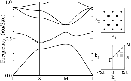
FIG. 1.: Band-gap structure of the $E$-polarized light in a 2D reduced-symmetry photonic crystal with $r_{1}=0.1a$, $r_{2}=0.05a$, and $\epsilon=11.4$. Full lines are calculated directly from Eq. (1) by MIT Photonic-Bands program [11], whereas dashed line is found from linearized Eq. (5). The top right inset shows a cross-sectional view of the photonic crystal and the bottom right inset shows the corresponding Brillouin zone.

A low-intensity light cannot propagate through a photonic crystal if the light frequency falls into a band gap. However, it has been recently suggested [5] that in the case of a 2D periodic medium with a Kerr-type nonlinear material, high-intensity light with the frequency inside the photonic gap can propagate in the form of finite energy solitary waves — 2D gap solitons. Such solitary waves were analyzed in the framework of the coupled-mode continuum-limit equations valid for a weak modulation of the dielectric constant $\epsilon(\mathchoice{{\hbox{\boldmath$\displaystyle x$}}}{{\hbox{\boldmath$\textstyle x$}}}{{\hbox{\boldmath$\scriptstyle x$}}}{{\hbox{\boldmath$\scriptscriptstyle x$}}})$. However, in real photonic crystals the modulation of $\epsilon(\mathchoice{{\hbox{\boldmath$\displaystyle x$}}}{{\hbox{\boldmath$\textstyle x$}}}{{\hbox{\boldmath$\scriptstyle x$}}}{{\hbox{\boldmath$\scriptscriptstyle x$}}})$ is comparable to its average value, so that the existence and stability of localized modes in such structures is still an open problem.

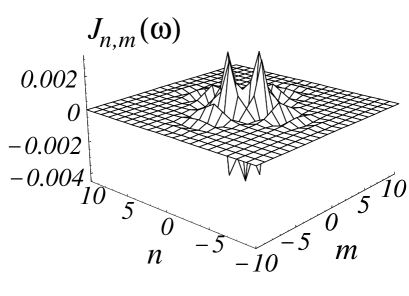
FIG. 2.: Coupling coefficients $J_{n,m}(\omega)$ for the photonic crystal depicted in Fig. 1. The frequency $\omega=0.4456\times 2\pi c/a$ is in the lower band gap. The contribution from $J_{0,0}=0.039$ is not shown.

More specifically, the coupled-mode equations are valid if and only if the band gap $\Delta\omega^{2}$ is vanishingly small, i. e. $\Delta\omega^{2}\sim A^{2}$ where $A$ is an effective amplitude of the mode that is treated in the multi-scale asymptotic expansions [12] as a small parameter. If we apply this model to describe nonlinear modes in a wider gap (see, e.g., discussions in Ref. [12]), we obtain a 2D cubic nonlinear Schrödinger (NLS) equation known to possess no stable localized solutions. Moreover, 2D localized modes of the coupled-mode equations are expected to possess an oscillatory instability recently discovered for a broad class of 1D coupled-mode equations [13]. Thus, it is clear that, if nonlinear localized modes do exist in realistic PBG materials, their existence and stability should be associated with different physical mechanisms not accounted for by simplified continuum coupled-mode models.

To study the nonlinear modes in such structures, we consider the nonlinear rods of small radius $r_{2}$ as “defects” embedded into the linear photonic crystal formed by a square lattice of the rods of larger radius $r_{1}$ (”diatomic crystal”). Then, writing the dielectric constant $\epsilon(\mathchoice{{\hbox{\boldmath$\displaystyle x$}}}{{\hbox{\boldmath$\textstyle x$}}}{{\hbox{\boldmath$\scriptstyle x$}}}{{\hbox{\boldmath$\scriptscriptstyle x$}}})$ as a sum of two periodic terms, $\epsilon(\mathchoice{{\hbox{\boldmath$\displaystyle x$}}}{{\hbox{\boldmath$\textstyle x$}}}{{\hbox{\boldmath$\scriptstyle x$}}}{{\hbox{\boldmath$\scriptscriptstyle x$}}})=\epsilon_{1}(\mathchoice{{\hbox{\boldmath$\displaystyle x$}}}{{\hbox{\boldmath$\textstyle x$}}}{{\hbox{\boldmath$\scriptstyle x$}}}{{\hbox{\boldmath$\scriptscriptstyle x$}}})+\epsilon_{2}(\mathchoice{{\hbox{\boldmath$\displaystyle x$}}}{{\hbox{\boldmath$\textstyle x$}}}{{\hbox{\boldmath$\scriptstyle x$}}}{{\hbox{\boldmath$\scriptscriptstyle x$}}}\,|\,E)\,,$ where $\epsilon_{1}(\mathchoice{{\hbox{\boldmath$\displaystyle x$}}}{{\hbox{\boldmath$\textstyle x$}}}{{\hbox{\boldmath$\scriptstyle x$}}}{{\hbox{\boldmath$\scriptscriptstyle x$}}})$ describes the linear photonic crystal and $\epsilon_{2}(\mathchoice{{\hbox{\boldmath$\displaystyle x$}}}{{\hbox{\boldmath$\textstyle x$}}}{{\hbox{\boldmath$\scriptstyle x$}}}{{\hbox{\boldmath$\scriptscriptstyle x$}}}\,|\,E)$ corresponds to a lattice of nonlinear defect rods, one can present Eq. (2) in the form [6, 7]

$$E(\mathchoice{{\hbox{\boldmath$\displaystyle x$}}}{{\hbox{\boldmath$\textstyle x$}}}{{\hbox{\boldmath$\scriptstyle x$}}}{{\hbox{\boldmath$\scriptscriptstyle x$}}},t\,|\,\omega)=\int d^{2}\mathchoice{{\hbox{\boldmath$\displaystyle y$}}}{{\hbox{\boldmath$\textstyle y$}}}{{\hbox{\boldmath$\scriptstyle y$}}}{{\hbox{\boldmath$\scriptscriptstyle y$}}}\,\,\,G(\mathchoice{{\hbox{\boldmath$\displaystyle x$}}}{{\hbox{\boldmath$\textstyle x$}}}{{\hbox{\boldmath$\scriptstyle x$}}}{{\hbox{\boldmath$\scriptscriptstyle x$}}},\mathchoice{{\hbox{\boldmath$\displaystyle y$}}}{{\hbox{\boldmath$\textstyle y$}}}{{\hbox{\boldmath$\scriptstyle y$}}}{{\hbox{\boldmath$\scriptscriptstyle y$}}}\,|\,\omega)\,\hat{\cal L}\,E(\mathchoice{{\hbox{\boldmath$\displaystyle y$}}}{{\hbox{\boldmath$\textstyle y$}}}{{\hbox{\boldmath$\scriptstyle y$}}}{{\hbox{\boldmath$\scriptscriptstyle y$}}},t\,|\,\omega)\;,$$ (3)

where we introduce the Green function $G(\mathchoice{{\hbox{\boldmath$\displaystyle x$}}}{{\hbox{\boldmath$\textstyle x$}}}{{\hbox{\boldmath$\scriptstyle x$}}}{{\hbox{\boldmath$\scriptscriptstyle x$}}},\mathchoice{{\hbox{\boldmath$\displaystyle y$}}}{{\hbox{\boldmath$\textstyle y$}}}{{\hbox{\boldmath$\scriptstyle y$}}}{{\hbox{\boldmath$\scriptscriptstyle y$}}}\,|\,\omega)$ of the linear photonic crystal (see, e.g., Ref. [14] for its properties) and the linear operator

$$\hat{\cal L}=\left(\frac{\omega}{c}\right)^{2}\epsilon_{2}(\mathchoice{{\hbox{\boldmath$\displaystyle x$}}}{{\hbox{\boldmath$\textstyle x$}}}{{\hbox{\boldmath$\scriptstyle x$}}}{{\hbox{\boldmath$\scriptscriptstyle x$}}}\,|\,E)+2\,i\,\epsilon(\mathchoice{{\hbox{\boldmath$\displaystyle x$}}}{{\hbox{\boldmath$\textstyle x$}}}{{\hbox{\boldmath$\scriptstyle x$}}}{{\hbox{\boldmath$\scriptscriptstyle x$}}})\frac{\omega}{c^{2}}\frac{\partial}{\partial t}\;.$$ (4)

Now, using the indices $n$ and $m$ for numbering the nonlinear rods in the $x_{1}$ and $x_{2}$ directions, we can describe their positions by the vectors $\mathchoice{{\hbox{\boldmath$\displaystyle x$}}}{{\hbox{\boldmath$\textstyle x$}}}{{\hbox{\boldmath$\scriptstyle x$}}}{{\hbox{\boldmath$\scriptscriptstyle x$}}}_{n,m}=n\,\mathchoice{{\hbox{\boldmath$\displaystyle a$}}}{{\hbox{\boldmath$\textstyle a$}}}{{\hbox{\boldmath$\scriptstyle a$}}}{{\hbox{\boldmath$\scriptscriptstyle a$}}}_{1}+m\,\mathchoice{{\hbox{\boldmath$\displaystyle a$}}}{{\hbox{\boldmath$\textstyle a$}}}{{\hbox{\boldmath$\scriptstyle a$}}}{{\hbox{\boldmath$\scriptscriptstyle a$}}}_{2}$, where $\mathchoice{{\hbox{\boldmath$\displaystyle a$}}}{{\hbox{\boldmath$\textstyle a$}}}{{\hbox{\boldmath$\scriptstyle a$}}}{{\hbox{\boldmath$\scriptscriptstyle a$}}}_{1}$ and $\mathchoice{{\hbox{\boldmath$\displaystyle a$}}}{{\hbox{\boldmath$\textstyle a$}}}{{\hbox{\boldmath$\scriptstyle a$}}}{{\hbox{\boldmath$\scriptscriptstyle a$}}}_{2}$ are the primitive lattice vectors of the 2D photonic crystal, and write

$$\epsilon_{2}(\mathchoice{{\hbox{\boldmath$\displaystyle x$}}}{{\hbox{\boldmath$\textstyle x$}}}{{\hbox{\boldmath$\scriptstyle x$}}}{{\hbox{\boldmath$\scriptscriptstyle x$}}}\,|\,E)=\left\{\epsilon_{2}^{(0)}+\chi^{(3)}|E(\mathchoice{{\hbox{\boldmath$\displaystyle x$}}}{{\hbox{\boldmath$\textstyle x$}}}{{\hbox{\boldmath$\scriptstyle x$}}}{{\hbox{\boldmath$\scriptscriptstyle x$}}},t\,|\,\omega)|^{2}\right\}\sum_{n,m}\theta(\mathchoice{{\hbox{\boldmath$\displaystyle x$}}}{{\hbox{\boldmath$\textstyle x$}}}{{\hbox{\boldmath$\scriptstyle x$}}}{{\hbox{\boldmath$\scriptscriptstyle x$}}}-\mathchoice{{\hbox{\boldmath$\displaystyle x$}}}{{\hbox{\boldmath$\textstyle x$}}}{{\hbox{\boldmath$\scriptstyle x$}}}{{\hbox{\boldmath$\scriptscriptstyle x$}}}_{n,m})\;,$$

where $\theta(\mathchoice{{\hbox{\boldmath$\displaystyle x$}}}{{\hbox{\boldmath$\textstyle x$}}}{{\hbox{\boldmath$\scriptstyle x$}}}{{\hbox{\boldmath$\scriptscriptstyle x$}}})=1$ for $|\mathchoice{{\hbox{\boldmath$\displaystyle x$}}}{{\hbox{\boldmath$\textstyle x$}}}{{\hbox{\boldmath$\scriptstyle x$}}}{{\hbox{\boldmath$\scriptscriptstyle x$}}}|\leq r_{2}$ and $\theta(\mathchoice{{\hbox{\boldmath$\displaystyle x$}}}{{\hbox{\boldmath$\textstyle x$}}}{{\hbox{\boldmath$\scriptstyle x$}}}{{\hbox{\boldmath$\scriptscriptstyle x$}}})=0$ otherwise. The parameter $\epsilon_{2}^{(0)}$ is the dielectric constant of the defect rods in the linear limit, while the term $\chi^{(3)}|E|^{2}$ takes into account a contribution due to the Kerr nonlinearity. If the radius $r_{2}$ of the defect rods is sufficiently small, the electric field $E(\mathchoice{{\hbox{\boldmath$\displaystyle x$}}}{{\hbox{\boldmath$\textstyle x$}}}{{\hbox{\boldmath$\scriptstyle x$}}}{{\hbox{\boldmath$\scriptscriptstyle x$}}},t\,|\,\omega)$ inside them is almost constant, and Eq. (3) can be approximated [6, 7] by the discrete nonlinear equation

$$i\sigma\frac{\partial}{\partial t}E_{n,m}-E_{n,m}$$ (5)

$$+\sum_{k,l}J_{n-k,\,m-l}(\omega)\left\{\epsilon_{2}^{(0)}+\chi^{(3)}|E_{k,l}|^{2}\right\}E_{k,l}=0\;,$$ (6)

for the amplitudes of the electric field $E_{n,m}(t\,|\,\omega)\equiv E(\mathchoice{{\hbox{\boldmath$\displaystyle x$}}}{{\hbox{\boldmath$\textstyle x$}}}{{\hbox{\boldmath$\scriptstyle x$}}}{{\hbox{\boldmath$\scriptscriptstyle x$}}}_{n,m},t\,|\,\omega)$ calculated at the defect rods. The parameter $\sigma$ and the coupling coefficients

$$J_{n,m}(\omega)=\left(\frac{\omega}{c}\right)^{2}\int_{r_{2}}d^{2}\mathchoice{{\hbox{\boldmath$\displaystyle y$}}}{{\hbox{\boldmath$\textstyle y$}}}{{\hbox{\boldmath$\scriptstyle y$}}}{{\hbox{\boldmath$\scriptscriptstyle y$}}}\,\,\,G(\mathchoice{{\hbox{\boldmath$\displaystyle x$}}}{{\hbox{\boldmath$\textstyle x$}}}{{\hbox{\boldmath$\scriptstyle x$}}}{{\hbox{\boldmath$\scriptscriptstyle x$}}}_{0,0},\mathchoice{{\hbox{\boldmath$\displaystyle x$}}}{{\hbox{\boldmath$\textstyle x$}}}{{\hbox{\boldmath$\scriptstyle x$}}}{{\hbox{\boldmath$\scriptscriptstyle x$}}}_{n,m}+\mathchoice{{\hbox{\boldmath$\displaystyle y$}}}{{\hbox{\boldmath$\textstyle y$}}}{{\hbox{\boldmath$\scriptstyle y$}}}{{\hbox{\boldmath$\scriptscriptstyle y$}}}\,|\,\omega)$$ (7)

are determined by the Green function $G(\mathchoice{{\hbox{\boldmath$\displaystyle x$}}}{{\hbox{\boldmath$\textstyle x$}}}{{\hbox{\boldmath$\scriptstyle x$}}}{{\hbox{\boldmath$\scriptscriptstyle x$}}},\mathchoice{{\hbox{\boldmath$\displaystyle y$}}}{{\hbox{\boldmath$\textstyle y$}}}{{\hbox{\boldmath$\scriptstyle y$}}}{{\hbox{\boldmath$\scriptscriptstyle y$}}}\,|\,\omega)$ which we calculate numerically by the FDTD method [15] with the spatial step $\Delta x=0.01$ to $0.03$ and time step $\Delta t=0.005$, for the lattice $24a\times 24a$. The Green function and, therefore, the coupling coefficients $J_{n,m}(\omega)$ in 2D photonic crystals are usually long-ranged functions. For instance, for the case of Fig. 2 we obtain $J_{n,0}\simeq 0.012\,(-1)^{n}\,\exp(-0.66\,|n|)$ for $n\geq 2$, so that one should take into account the interaction between at least 10 neighbors to achieve a good accuracy for the spectrum. By this means, Eq. (5) is a nontrivial long-range generalization of the 2D discrete NLS equations extensively studied during the last decade [16]. We have checked the accuracy of the approximation provided by Eq. (5) by solving it in the linear limit. The low-frequency part of this dependence for $\epsilon_{2}^{(0)}=11.4$ is depicted in Fig. 1 by a dashed line; it has a minimum at $\omega=0.446\times 2\pi c/a$ being in a good agreement with the band edge calculated directly from Eq. (2). This lends a support to the validity of Eq. (5) and allows us to use this discrete model for studying nonlinear properties.

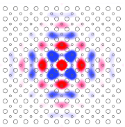
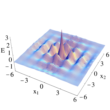
FIG. 3.: (Color) Top and 3D views of a nonlinear localized mode in the 2D photonic crystal shown in Fig. 1 ($\omega=0.442\times 2\pi c/a$).

Stationary nonlinear localized modes have been calculated numerically by the Newton-Raphson iteration scheme on the lattice $170a\times 170a$. Assuming that the linear rods are made from GaAs whereas the nonlinear rods are made from some nonlinear material (which we do not specify varying $\epsilon_{2}^{(0)}$), we find a continuous family of nonlinear localized modes, and a typical example [smoothed by continuous optimization for Eq. (3)] of such a mode is shown in Fig. 3. At first glance, this mode can be regarded as a donor state created by a single defect rod with larger dielectric constant. However, in the nonlinear case the mode stability becomes a critical issue. It can be determined from the so-called Vakhitov-Kolokolov stability criterion extended to the 2D discrete NLS models in Ref. [17]. According to this criterion, the nonlinear localized states with $dQ/d\omega<0$ are stable, and they are unstable otherwise. Here

$$Q(\omega)=\sum_{n,m}|E_{n,m}|^{2}\;,$$ (8)

is the conserved mode power proportional to the energy of the electric field accumulated in the nonlinear localized mode.

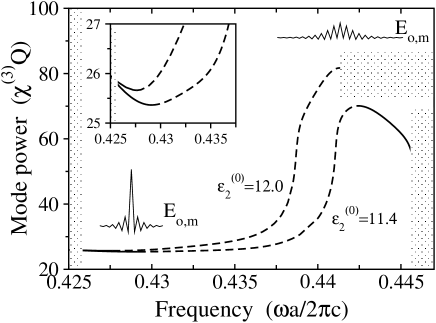
FIG. 4.: Power $Q$ vs. frequency $\omega$ for the 2D nonlinear localized modes in the photonic crystal of Fig. 1 with two different $\epsilon_{2}^{(0)}$. Solid lines – stable modes, dashed lines – unstable modes. Grey areas show the projected band structure of the crystal. Insets show typical profiles of stable modes, and an enlarged part of the power dependence.

As is well known (see, e.g., Refs. [17]) in the 2D discrete cubic NLS equation, only high-amplitude localized modes are stable, whereas no stable modes exist in the continuum limit. For our model, the high-amplitude modes are also stable (see inset in Fig. 4), but they are not accessible under realistic conditions: To excite such modes one should increase the refractive index at the mode center in more than 2 times. Thus, for realistic conditions and relatively small values of $\chi^{(3)}$, only low-amplitude localized modes become a subject of much interest since they can be excited in experiment. However, such modes in unbounded 2D NLS models are always unstable and either collapse or spread out [16]. Here we reveal that, in a sharp contrast to the 2D discrete NLS models discussed earlier in various applications, the low-amplitude localized modes of Eq. (5) can be stabilized due to nonlinear long-range dispersion inherent to the photonic crystals. It should be emphasized that such stabilization does not occur in the models with only linear long-range dispersion [16].

In order to gain a better insight into the stabilization mechanism, we have carried out the studies of Eq. (5) for the exponentially decaying coupling coefficients $J_{n,m}$. Our results show that the most important factor which determines stability of the low-amplitude localized modes is a ratio of the coefficients at the local nonlinearity ($\sim J_{0,0}$) and the nonlinear dispersion ($\sim J_{0,1}$). If the coupling coefficients $J_{n,m}$ decrease with the distances $n$ and $m$ rapidly, the low-amplitude modes of Eq. (5) with $\epsilon_{2}^{(0)}=11.4$ are essentially stable for $J_{0,0}/J_{0,1}\lesssim 13$. However, this estimation is usually lowered because the stabilization is favored by the presence of long-range interactions.

It should be mentioned that the stabilization of low-amplitude 2D localized modes is not inherent to all types of nonlinear photonic crystals. On the contrary, the photonic crystals must be carefully designed to support stable low-amplitude nonlinear modes. For example, in the photonic crystal considered above such modes are stable at least for $11<\epsilon_{2}^{(0)}<12$, however they become unstable for $\epsilon_{2}^{(0)}\geq 12$ (see Fig. 4). The stability of these modes can also be controlled by varying $r_{2}$, $r_{1}$, or $\epsilon_{1}$. Thus, experimental observation of the nonlinear localized modes would require not only the use of photonic materials with a relatively large nonlinear refractive index (such as GaAs/AlAs periodic structures [18] or polymer PBG crystals [19]), but also a fine adjustment of the parameters of the photonic crystal. The latter can be achieved, in principle, by employing the surface coupling technique [20] that is able to provide coupling to specific points of the dispersion curve, opening up a very straightforward way to access nonlinear effects.

In conclusion, we have developed a consistent theory of nonlinearity-induced self-trapping effects in 2D nonlinear photonic crystals and predicted the possibility of the energy localization near the bandgap edge in the form of stable 2D nonlinear localized modes.

Yuri Kivshar thanks V. Astratov, K. Busch, S. John, A. McGurn, M. Scalora, and C. Soukoulis for encouraging comments and discussions. Serge Mingaleev is indebted to Yu.B. Gaididei for useful remarks. The work has been partially supported by the Australian Research Council and the Performance and Planning Foundation grant of the Institute of Advanced Studies.

REFERENCES

• [1] J. D. Joannoupoulos, R. B. Meade, and J. N. Winn, Photonic Crystals (Princeton University Press, 1995).
• [2] See, e.g., K. Busch and S. John, Phys. Rev. Lett. 83, 967 (1999), and discussions therein.
• [3] See, e.g., M. Scalora et al., Phys. Rev. Lett. 73, 1368 (1994); P. Tran, Phys. Rev. B 52, 10673 (1995).
• [4] W. Chen and D. L. Mills, Phys. Rev. Lett. 58, 160 (1987); D. N. Christodoulides and R. I. Joseph, Phys. Rev. Lett. 62, 1746 (1989); see also the review paper: C. M. de Sterke and J. E. Sipe, in Progress in Optics XXXIII, edited by E. Wolf (Elsevier, Amsterdam, 1994), p. 203.
• [5] S. John and N. AkΓΆzbek, Phys. Rev. Lett. 71, 1168 (1993); Phys. Rev. E 57, 2287 (1998).
• [6] A. R. McGurn, Phys. Lett. A 260, 314 (1999).
• [7] S. F. Mingaleev et al., Phys. Rev. E 62, 5777 (2000).
• [8] See, e.g., A. J. Sievers and S. Takeno, Phys. Rev. Lett. 61, 970 (1988); S. Flach and C. R. Willis, Phys. Rep. 295, 181 (1998).
• [9] H. S. Eisenberg et al., Phys. Rev. Lett. 81, 3383 (1998); B. I. Swanson et al., Phys. Rev. Lett. 82, 3288 (1999); U. T. Schwarz et al., Phys. Rev. Lett. 83, 223 (1999); E. Trias et al., Phys. Rev. Lett. 84, 741 (2000); P. Binder et al., Phys. Rev. Lett. 84, 745 (2000).
• [10] C. M. Anderson and K. P. Giapis, Phys. Rev. Lett. 77, 2949 (1996); Phys. Rev. B 56, 7313 (1997).
• [11] S. G. Johnson, http://ab-initio.mit.edu/mpb/
• [12] Yu. S. Kivshar et al., Int. J. Mod. Phys. B 9, 2963 (1995).
• [13] I. V. Barashenkov et al., Phys. Rev. Lett. 80, 5117 (1998); A. De Rossi et al., Phys. Rev. Lett. 81, 85 (1998).
• [14] A.Β A. Maradudin and A.Β R. McGurn, in Photonic Band Gaps and Localization, NATO ASI Series B 308, Ed. C.Β M. Soukoulis (Plenum Press, New York, 1993), p. 247.
• [15] A.Β J. Ward and J.Β B. Pendry, Phys. Rev. B 58, 7252 (1998).
• [16] See, e.g., V.Β K. Mezentsev et al., JETP Lett. 60, 829 (1994); S. Flach et al., Phys. Rev. Lett. 78, 1207 (1997); P.Β L. Christiansen et al., Phys. Rev. B 57, 11303 (1998).
• [17] E.Β W.Β Laedke et al., JETP Lett. 62, 677 (1995); Phys. Rev. E 52, 5549 (1995); Yu. B. Gaididei et al., Phys. Rev. B 55, R13365 (1997).
• [18] P. Millar et al., Opt. Lett. 24, 685 (1999); A.A. Helmy et al., Opt. Lett. 25, 1370 (2000).
• [19] S. Shoji and S. Kawata, Appl. Phys. Lett. 76, 2668 (2000).
• [20] V. N. Astratov et al., Phys. Rev. B 60, R16255 (1999).