Effect of Angular momentum on equilibrium properties of a self–gravitating system

Abstract

The microcanonical properties of a two dimensional system of $N$ classical particles interacting via a smoothed Newtonian potential as a function of the total energy $E$ and the total angular momentum $L$ are discussed. The two first moments of the distribution of the linear momentum of a given particle at a fixed position show that, (a) in average the system rotates like a solid body (b) the equipartition theorem has to be corrected by a term proportional to the square of the fluctuations of the inertial momentum of the system. In order to estimate suitable observables a numerical method based on an importance sampling algorithm is presented. The entropy surface $S$ shows a negative specific heat region at fixed $L$ for all $L$. Observables probing the average mass distribution are used to understand the link between thermostatistical properties and the spatial distribution of particles. In order to define a phase in non–extensive system we introduce a more general observable than the one proposed by Gross and Votyakov [Eur. Phys. J. B 15, 115 (2000)]. This observable is the sign of the largest eigenvalue of the entropy surface curvature. If it is negative then the system is in a pure phase; if it is positive then the system undergoes a first order phase transition. At large $E$ the gravitational system is in a homogeneous gas phase. At low $E$ there are several collapse phases; at $L=0$ there is a single cluster phase and for $L\neq 0$ there are several phases with two clusters, the relative size of the clusters depends on $L$. All these pure phases are separated by first order phase transition regions. The signal of critical behaviour emerges at different points of the parameter space $\left(E,L\right)$. We also discuss the ensemble introduced in a recent pre–print by Klinko and Miller; this ensemble is the canonical analogue of the one at constant energy and constant angular momentum, i.e. it is defined at constant temperature and constant angular velocity. We show that a huge loss of informations appears if we treat the system as a function of intensive parameters: besides the known non–equivalence at first order phase transitions, there exit in the microcanonical ensemble some values of the temperature and the angular velocity for which the corresponding canonical ensemble does not exist, i.e. the partition sum diverges.

I Introduction

The thermostatistical properties of systems of $N$ classical particles under a long–range attractive potential have been extensively studied since the seminal work of Antonov [1], [2, 3, 4, 5, 6, 7]. One of their more specific and interesting properties is that they are unstable for all $N$ [2] and therefore not thermodynamically extensive, i.e. they exhibit negative specific heat regions even when the system is composed by a very large number of particles.

It is quite natural to ask whether the total angular momentum $L$, which is an integral of motion for systems of relevance in the astrophysical context, plays a non–trivial role on the equilibrium properties of these systems. Indeed $L$ is considered as an important parameter in order to understand the physics of systems like galaxies [8, 9, 10]; globular clusters [11, 12, 13, 14, 15]; molecular clouds in multifragmentation regime [16, 17] which might eventually lead to stellar formation [18, 19, 20, 21, 22, 23, 24].

Previous works have already studied the effect of $L$ in the mean field limit with a simplified potential and imposing a spherical symmetry [14, 25]; or at $L=0$ [13].

Our work, presented in this paper, is an attempt to overcome some of these approximations.

Thermodynamical equilibrium does not exist for Newtonian self–gravitating systems, due both to evaporation of stars (the systems are not self–bounded) and short distance singularity in the interaction potential. However there exists intermediate stages where these two effects might be neglected and a quasi–equilibrium state might be reached (dynamical issues like ergodicity, mixing or “approach to equilibrium” [7, 26, 27] are not considered in this paper). In order to make the existence of equilibrium configurations possible we have, first, to bound the system in an artificial box and, second, to add a short distance cutoff to the potential. The latter point can be seen as an attempt to take into account the appearance of new physics at very short distances (about the influence of this short cut see [28, 29]). Another way to avoid the difficulties due to the short distance singularity is to describe the function of distribution of the “stars” within a Fermi–Dirac statistic [3, 30].

The box breaks the translational symmetry of the system, therefore the total linear momentum $P$ and angular momentum $L$ are not conserved. Nevertheless we assume that the equilibration time is smaller than the characteristic time after which the box plays a significant role [13, 25]. Therefore $P$ and $L$ are considered as (quasi–)conserved quantities. We put the center of the box at the center of mass $R_{CM}$ which is also set to be the center of the coordinates. Therefore $P=0$.

As already mentioned, self–gravitating systems are non–extensive and a statistical description based on their intensive parameters should be taken with caution since the different statistical ensembles are only equivalent at the thermodynamical limit far from first order transitions (see Sec. III D). Moreover, this limit is required in order to define phases and phase transitions if one fixes the intensive parameters [31]. In contrast, the microcanonical ensemble (ME) does not require this limit, it allows a classification of phase transitions for finite size systems [32, 33]. Hence the considered system is studied within the natural ME framework.

In order to perform the computation in a reasonable time we have to consider a two dimensional system.

The paper is organized as follow: In section II we recall the analytical expressions for entropy and its derivatives (Sec. II A), clarify the definition of phase transitions for non–extensive systems proposed in [32] (Sec. II B), discuss the two first moments of the distribution of the linear momentum of a given particle at a fixed position (Sec. II C), and present a numerical method based on an importance sampling algorithm in order to estimate suitable observables (Sec. II D). Numerical results are presented in section III; the link between the average mass distribution and the thermostatistical properties is made in Sec. III B. In Sec. III C we use the definition of phase introduced in Sec. II B to draw the phase diagram of the self–gravitating system as a function of its energy $E$ and angular momentum $L$. We discuss the ensemble introduced in [14]; therein this ensemble is used to treat another model of rotating and self–gravitating system. This ensemble is a function of the (intensive) variables conjugate of $E$ and $L$. For our model we show how the predictions using this ensemble are inaccurate and misleading (Sec. III D). Results are summarized and discussed in section IV.

II Microcanonical properties

A Microcanonical definitions

Consider a system of $N$ classical particles on a disk of radius $R$ whose interaction is described by a Plummer softened potential [34, 35]

$$\varphi_{ij}=-\frac{Gm_{i}m_{j}}{\sqrt{s^{2}+(\mbox{\boldmath$q$}_{i}-\mbox{\boldmath$q$}_{j})^{2}}},$$ (1)

where $m_{i}$ and $\mbox{\boldmath$q$}_{i}=\{q_{i}^{1},q_{i}^{2}\}$ are the mass and position of particle $i$ respectively, $s$ is the softening length and $G$ is the gravitational constant. The fixed total energy $E$ is described by the Hamiltonian

$${\cal H}=\sum_{i}\frac{\mbox{\boldmath$p$}_{i}^{2}}{2m_{i}}+\varphi(\mbox{\boldmath$q$}),$$ (2)

where $\mbox{\boldmath$p$}_{i}=\{p_{i}^{1},p_{i}^{2}\}$ is the linear momentum of particle $i$, $\varphi=\sum_{i<j}\varphi_{ij}$ and $q$ is a $2N$–dimensional vector whose coordinates are $\{\mbox{\boldmath$q$}_{1},\ldots,\mbox{\boldmath$q$}_{N}\}$, representing the spatial configuration and is an element of the spatial configuration space $V_{c}$, $\mbox{\boldmath$q$}\in V_{c}\subset{\mathbb{R}}^{2N}$.

The entropy $S$ is given through the Boltzmann’s principle (the Boltzmann constant is set to 1)

$$S(E,L,N)=\log\left(W(E,L,N)\right),$$ (3)

where $W(E,L,N)$ is the volume of the accessible phase–space at $E$, $L$ and $N$ fixed (under the assumptions given in I)

$$W\big{(}E,L,N\big{)} = \frac{1}{N!}\int\prod_{i=1}^{N}\left(\frac{d\mbox{\boldmath$p$}_{i}\-d\mbox{\boldmath$q$}_{i}}{(2\pi\hbar)^{2}}\right)\delta\big{(}E-{\cal H}\big{)}\delta^{(2)}\big{(}\sum_{i}\mbox{\boldmath$p$}_{i}\big{)}$$ (5)

$$\times\delta\big{(}L-\sum_{i}\mbox{\boldmath$q$}_{i}\times\mbox{\boldmath$p$}_{i}\big{)}\delta^{(2)}\big{(}\sum_{i}\mbox{\boldmath$q$}_{i}\big{)},$$

where $\mbox{\boldmath$q$}_{i}\times\mbox{\boldmath$p$}_{i}=q_{i}^{1}p_{i}^{2}-q_{i}^{2}p_{i}^{1}$. After integration over the momenta Eq. (5) becomes [25, 36]

$$W\big{(}E,L,N\big{)}={\cal C}\int_{V_{c}}d\mbox{\boldmath$q$}\>\frac{1}{\sqrt{I}}E_{r}^{N-5/2},$$ (6)

where ${\cal C}=\frac{(2\pi)^{(N-3/2)}\prod_{i}m_{i}}{(2\pi\hbar)^{2N}N!(\sum_{i}m_{i})\Gamma(N-3/2)}$ is a constant, $I=\sum_{i}m_{i}\mbox{\boldmath$q$}_{i}^{2}$ is the inertial momentum and $E_{r}=E-\frac{L^{2}}{2I}-\varphi$ the remaining energy . From the point of view of the remaining energy, if $L\neq 0$ we can already notice that the equilibrium properties are the results of a competition between two terms; the rotational energy $\frac{L^{2}}{2I}$ and the potential energy $\varphi$. The former tries to drive the particles away from the center of mass in order to increase $I$ whereas the latter tries to group the particles together in order to decrease $\varphi$, but since the center of mass is fixed this will lead to a concentration of particles near the center and consequently will decrease $I$.

The microcanonical temperature $T$ is defined by

$$\frac{1}{T}=\beta\equiv\frac{\partial S}{\partial E}=\langle\frac{N-5/2}{E_{r}}\rangle,$$ (7)

where $\langle\cdot\rangle$ is the microcanonical average

$$\langle{\cal O}\rangle=\frac{{\cal C}}{W}\int_{Vc}d\mbox{\boldmath$r$}\frac{{\cal O}\left(\mbox{\boldmath$r$}\right)}{\sqrt{I}}E_{r}^{N-5/2}.$$ (8)

The angular velocity $\omega$ is defined as minus the conjugate force of $L$ times T [37]

$$-\omega\equiv\frac{1}{\beta}\frac{\partial S}{\partial L}=-\frac{\langle\frac{L}{I}E_{r}^{-1}\rangle}{\langle E_{r}^{-1}\rangle}$$ (9)

We also define $\gamma\beta$ has the conjugate of $L^{2}$:

$$\gamma\beta \equiv \frac{\partial S}{\partial L^{2}}=-\langle\frac{1}{2I}\frac{N-5/2}{E_{r}}\rangle,$$ (10)

$$\omega = 2L\gamma.$$ (11)

B Phase and phase transitions

For small or self–gravitating systems a phase (or a phase transition) can not be defined in the usual way using for example the Lee and Yang singularities [31] since these singularities show up only at the thermodynamical limit. Invoking the thermodynamical limit when studying small systems washses out all the finite size effects that may lead to new phenomena, (e.g. isomerisation of metallic clusters [38], multifragmentation of nuclei [39]) and for self–gravitating systems the thermodynamical limit does not exist. Hereafter, we will call “Small systems”, those where the range of the forces is of the order of the system size (e.g. metallic clusters, nuclei and self–gravitating systems) and also systems without proper thermodynamical limit (e.g. unstable systems [40]).

In a recent paper [32] definitions for pure phases and phase transitions (first and second kind) based on the local topology of the microcanonical entropy surface has been proposed. In the following we first fix some notations and then recall the definitions.

Consider the microcanonical ensemble (ME) of an isolated physical system. Its associated entropy $S(X)$ is a function of ${\cal N}$ “extensive” dynamical conserved quantities $X=\{X^{1},\ldots,X^{\cal N}\}$. Note that $X$ may not contain all the dynamical conserved quantities and for simplicity all these parameters are considered as being continuous. The Jacobian of $S(X=X_{0})$ is noted by $J_{S}(X_{0})=\|\frac{\partial^{2}S}{\partial X^{i}\partial X^{j}}\|_{X_{0}}$, its eigenvalues are $\{\lambda_{1},\ldots,\lambda_{\cal N}\}$ where $\lambda_{1}\geq\lambda_{2}\geq\ldots\geq\lambda_{\cal N}$ and the determinant of $J_{S}(X)$ is $D_{S}=\lambda 1\cdots\lambda_{\cal N}$.

In [32] phase transitions are defined “by the points and regions of non–negative curvature of the entropy surface […] as a function of the mechanical quantities”. Therein the sign of $D_{S}$ is put forward as a measure the concavity of $S$ (its negative curvature) so that at first order phase transition

$${\rm sign}\left(D_{S}\right)={\rm sign}\left((-1)^{{\cal N}+1}\right).$$ (12)

Though this condition is necessary it is not sufficient in the general case. In fact $S$ is a non–concave function at $X_{0}$ if

$$\lambda_{1}\geq 0,$$ (13)

i.e. if at least one eigenvalue of $J_{S}$ is non–negative. Note that in the two dimensional example model studied in [32] in order to illustrate the definition (12), $\lambda_{2}$ is always negative therefore the sign of $D_{S}$ is simply minus the one of $\lambda_{1}$, and the conditions (12) and (13) are equivalent.

By using ${\rm sign}(\lambda_{1})$, one can somewhat extend or clarify the classification of phase transitions in non–extensive systems when the entropy is a function of ${\cal N}\geq 1$ variables for any set of the parameters $X_{0}$

• A single pure phase if $\lambda_{1}(X_{0})<0$.

• A first order phase transition if $\lambda_{1}(X_{0})>0$. As mentioned in [32, 41] the depth of the associated entropy intruder is a measure of the intra–phase surface tension; how to define and to measure these depth when ${\cal N}>1$ will be discussed elsewhere. Note that some eigenvalues might still be negative although $\lambda_{1}(X_{0})>0$ just like in the model presented in [32]. In this case “good” order parameters are linear combinations of the eigenvectors whose eigenvalues are positive.

• If $\lambda_{1}(X_{0})=0$ and $\lambda_{1}$ is the only zero eigenvalue and $\nabla_{{\bf v}_{1}}\lambda_{1}=0$, where ${\bf v}_{1}$ is the eigenvector associated with $\lambda_{1}$ then there is a second order phase transition at $X_{0}$.

• If several eigenvalues obey $\lambda_{i}=0$ and $\nabla_{{\bf v}_{i}}\lambda_{i}=0$ for $i=1,\ldots,n\leq{\cal N}$ then $X_{0}$ is a multicritical point.

C Momentum average and dispersion

In this section we derive the average and the dispersion of the linear momentum of a particle, we also compute its mean angular velocity and relate it to the one of the system as defined in Eq. (9).

The derivation of $\langle\mbox{\boldmath$p$}_{k}\rangle_{\mbox{\boldmath$q$}_{k}}$ the average momentum of particle $k$ at fixed position $\mbox{\boldmath$q$}_{k}$ (while the other particles are free) is similar to that of $W$. Details of the derivation can be found in Appendix A, and the result is

$$\langle\mbox{\boldmath$p$}_{k}\rangle_{\mbox{\boldmath$q$}_{k}}=L\langle I^{-1}\rangle_{\mbox{\boldmath$q$}_{k}}m_{k}\sum_{\alpha,\delta=1}^{2}\epsilon_{\alpha\delta}q_{k}^{\delta}{\bf e}_{\alpha},$$ (14)

where ${\bf\epsilon}$ is the antisymmetric tensor of rank 2 and ${\bf e}_{\alpha}$ the unit vector of coordinate $\alpha$. Equation (14) shows that $\langle\mbox{\boldmath$p$}_{k}\rangle_{\mbox{\boldmath$q$}_{k}}$ is a vector perpendicular to $\mbox{\boldmath$q$}_{k}$ whose module is a function of $\|\mbox{\boldmath$q$}_{k}\|$. In other words the orbit of a particle is in the mean circular (this result is expected since the system is rotationally symmetric). One can compute $\langle\omega_{k}\rangle_{\mbox{\boldmath$q$}_{k}}$ the mean angular velocity of $k$ at distance $\|\mbox{\boldmath$q$}_{k}\|$ by first considering $\langle L_{k}\rangle_{\mbox{\boldmath$q$}_{k}}$ the mean angular momentum of $k$ at distance $\|\mbox{\boldmath$q$}_{k}\|$

$$\langle L_{k}\rangle_{\mbox{\boldmath$q$}_{k}} \equiv \mbox{\boldmath$q$}_{k}\times\langle\mbox{\boldmath$p$}_{k}\rangle_{\mbox{\boldmath$q$}_{k}}$$ (15)

$$= L\langle I^{-1}\rangle_{\mbox{\boldmath$q$}_{k}}I_{k},$$ (16)

where $I_{k}=m_{k}\mbox{\boldmath$q$}_{k}^{2}$. The angular mean velocity of a particle on a circular orbit is classically linked to $\langle L_{k}\rangle_{\mbox{\boldmath$q$}_{k}}$ by

$$\langle L_{k}\rangle_{\mbox{\boldmath$q$}_{k}}=\langle\omega_{k}\rangle_{\mbox{\boldmath$q$}_{k}}I_{k}.$$ (17)

We can identify $\langle\omega_{k}\rangle_{\mbox{\boldmath$q$}_{k}}$ in (16) as

$$\langle\omega_{k}\rangle_{\mbox{\boldmath$q$}_{k}}=L\langle I^{-1}\rangle_{\mbox{\boldmath$q$}_{k}}.$$ (18)

The dependence of $\langle\omega\rangle_{\mbox{\boldmath$q$}_{k}}$ on $||\mbox{\boldmath$q$}_{k}||$ is of the order $1/N$ ($\langle I^{-1}\rangle_{\mbox{\boldmath$q$}_{k}}=\langle I^{-1}\rangle+{\cal O}(N^{-1})$), therefore for large $N$ we can write (see Eq. (9))

$$\langle\omega_{k}\rangle_{\mbox{\boldmath$q$}_{k}}\sim L\langle I^{-1}\rangle\approx\langle\omega\rangle.$$ (19)

For large $N$ the mean angular velocity is the same for all the particles at any distance from the center, in other words the system in the mean rotates like a solid body. Moreover $\langle\omega_{k}\rangle_{\mbox{\boldmath$q$}_{k}}$ corresponds to the thermostatistical angular velocity $\omega$ defined by Eq. (9). These are also classical results for extensive systems at low $L$[37, 42]. Note also that these results do not depend on the interaction potential $\varphi$.

The momentum dispersion $\sigma_{\mbox{\boldmath$p$}_{k}}$ can also be derived. Using Eq. (14) and Eq. (A8), we get for large $N$

$$\sigma_{\mbox{\boldmath$p$}_{k}}^{2} \equiv \langle\mbox{\boldmath$p$}_{k}^{2}\rangle_{\mbox{\boldmath$q$}_{k}}-\langle\mbox{\boldmath$p$}_{k}\rangle^{2}_{\mbox{\boldmath$q$}_{k}}$$ (20)

$$\sim 2\frac{m_{k}}{\beta}+I_{k}L^{2}m_{k}\left(\langle I^{-2}\rangle-\langle I^{-1}\rangle^{2}\right)$$ (21)

The second term of Eq. (21) is proportional to the square of the dispersion of $I^{-1}$ and to $\mbox{\boldmath$q$}_{k}^{2}$ ($I_{k}=m_{k}\mbox{\boldmath$q$}_{k}^{2}$). When this term vanishes relatively to the first one, e.g. when the fluctuations of $I^{-1}$ are small, or at high energy (low $\beta$) and low $L$, we recover the usual dispersion of the Maxwell–Boltzmann distribution. This term also gives a correction to the usual equipartition theorem; for large $N$

$$\langle E_{k}\rangle \equiv \frac{\sigma_{\mbox{\boldmath$p$}_{k}}^{2}}{2m_{k}}$$ (22)

$$\sim T+\frac{I_{k}L^{2}}{2}\left(\langle I^{-2}\rangle-\langle I^{-1}\rangle^{2}\right),$$ (23)

where $\langle E_{k}\rangle$ is the average internal kinetic energy (without the contribution from the collective rotational movement) of particle $k$. Again this correction is position–dependent via $I_{k}$. In the regimes where the fluctuations of the mass distribution can not be neglected in Eqs. (21) and (23) an estimation of the temperature based on the velocity dispersion would show that the temperature is smaller in the core than at the edge.

D Numerical method

From now on we set $m_{i}=m,\>\forall i=1,\cdots,N$ and use the following dimensionless variables: (i) $E\to\epsilon=\frac{ER}{Gm^{2}N^{2}}$; (ii) $L\to l^{2}=\Omega=\frac{L^{2}}{2Gm^{3}RN^{2}}$; (iii) $s\to\sigma=\frac{s}{R}$; (iv) $q\to r=\frac{q}{R}$; (v) $V_{c}\to v_{c}$; (vi) $\varphi\to\phi=\frac{R}{Gm^{2}N^{2}}\varphi=\frac{-1}{N^{2}}\sum_{i<j}\frac{1}{\sqrt{\sigma^{2}+(\mbox{\boldmath$r$}_{i}-\mbox{\boldmath$r$}_{j})^{2}}}$; (vii) $I\to I=\sum_{i}r_{i}^{2}$. The weight is now

$$W\left(\epsilon,\Omega\right)={\cal C^{\prime}}\int_{v_{c}}d\mbox{\boldmath$r$}\frac{1}{\sqrt{I}}\epsilon_{r}^{N-5/2},$$ (24)

where $\epsilon_{r}=\epsilon-\frac{\Omega}{I}-\phi$ is the dimensionles remaining energy and ${\cal C^{\prime}}$ a constant. Later on we no longer write this constant since it plays no significant role (it only shifts the entropy by $\log{{\cal C^{\prime}}}$). The derivatives of entropy ($\beta$, $\omega$, …) are now dimensionless quantities.

One usually estimates (24) by means of some Monte Carlo algorithm, updating the positions ${\bf q}$ by some small amount $\delta{\bf q}$ in order to get a good pass acceptance and using the configuration weight $W(\mbox{\boldmath$r$})=\frac{1}{\sqrt{I}}\epsilon_{r}^{N-5/2}$ in the Metropolis pass. Unfortunately this strategy does not really work (within a reasonable CPU–time), because the $2N$–dim configuration weight–landscape at fixed $\epsilon$ and $\Omega$ presents troughs and high peaks [43], so exploring the total configuration–space (or at least a subset containing the highest peaks) would take a very long, in practice infinite, time. This weight–landscape looks like the energy–landscape found in spin–glass systems.

The strategy we have adopted is described in the following. First we can rewrite (24)

$$W\left(\epsilon,\Omega\right)=\int dI\>d\phi\>Bg\left(I,\phi\right)\frac{1}{\sqrt{I}}\epsilon_{r}^{N-5/2},$$ (25)

where $Bg\left(I,\phi\right)=\int_{v_{c}}d\mbox{\boldmath$r$}\delta\left(I^{\prime}(\mbox{\boldmath$r$})-I\right)\delta\left(\phi^{\prime}(\mbox{\boldmath$r$})-\phi\right)$; $Bg\left(I,\phi\right)$ is the density of spatial configurations at given $I$ and $\phi$. Given $Bg$ we can compute $W$, $S$ and its derivatives for any $\epsilon$ and $\Omega$, e.g.

$$\gamma = \frac{1}{\beta}\frac{\partial S}{\partial\Omega}$$ (26)

$$= -\frac{N-5/2}{\beta}\frac{\int dI\>d\phi\>Bg\left(I,\phi\right)I^{-3/2}\epsilon_{r}^{N-7/2}}{W\left(\epsilon,\Omega\right)}.$$ (27)

The expectation value $\left\langle{\cal O}\right\rangle$ of an observable ${\cal O(\mbox{\boldmath$r$})}$ can be estimated if we know $Bg$ and $\left\langle{\cal O}\right\rangle_{I,\phi}$

$$\left\langle{\cal O}\right\rangle \equiv \frac{\int_{v_{c}}d\mbox{\boldmath$r$}\>{\cal O}(\mbox{\boldmath$r$})I^{-1/2}\epsilon_{r}^{N-5/2}}{\int_{v_{c}}d\mbox{\boldmath$r$}\>I^{-1/2}\epsilon_{r}^{N-5/2}}$$ (28)

$$= \frac{\int dI\>d\phi\>\left\langle{\cal O}\right\rangle_{I,\phi}Bg\left(I,\phi\right)I^{-1/2}\epsilon_{r}^{N-5/2}}{W\left(\epsilon,\Omega\right)},$$ (29)

where

$$\left\langle{\cal O}\right\rangle_{I,\phi}=\frac{\int_{v}d\mbox{\boldmath$r$}\>{\cal O}(\mbox{\boldmath$r$})\delta\left(I^{\prime}-I\right)\delta\left(\phi^{\prime}-\phi\right)}{Bg\left(I,\phi\right)}.$$ (30)

Now, we have to compute $Bg(I,\phi)$ and $\left\langle{\cal O}\right\rangle_{I,\phi}$. A priori $Bg(I,\phi)$ is highly peaked around the values of $I$ and $\phi$ that describe the gas (disordered) phase and should drop down to the edges. Nevertheless we need a good estimate of $Bg(I,\phi)$ for almost all values taken by $(I,\phi)$ even when $Bg(I,\phi)$ is very small comparing to its maximum. For example at small total energy $\epsilon$ only the part of $Bg(I,\phi)$ for which $\epsilon_{r}=\epsilon-\frac{\Omega^{2}}{I}-\phi>0$ will contribute to the integral (25).

In order to get a good estimate of $Bg$ we used an iterative scheme inspired by multicanonical algorithms [44, 45, 46, 47]. The usual multicanonical task is to compute the free energy as a function of the total energy. Here we have to compute $Bg$ as a function of $I$ and $\phi$. The updating scheme presented in [47] was used; one of the reason for this choice is that although it has been given for a one dimensional task it can be trivially extended to bi–variate problem. Furthermore we added a blocking mechanism: once we estimate that enough information has been collected on a given region of the parametric space $(I,\phi)$ then we tag it as “locked” so that it will not be visited during next iterations. This mechanism enables the program to spread more quickly over the parametric space and save computation time comparing to usual multicanonical algorithms. Details on this blocking mechanism will be given elsewhere [48].

FIG. 1.: Estimate of the density of state $Bg$ (a) and histogram of the visited states $C$ (b) for $I=3$ at different iteration steps $i$ of the multicanonical algorithm as a function of the potential energy $\phi$. Panel (a) shows how $Bg$ is built step by step; $Bg$ is an extremely peaked function, the log of the ratio between its maximum and its minimum is about $120$. Without the blocking mechanism (see text) $C_{i}$ would have been non null for all values of $\phi$ visited during previous steps $j<i$. In panel (b) we see that the algorithm does no longer visit “well–known” regions ($\phi\gtrsim-1.5$) already after four steps.

In the present paper we present results for $N=20$, and $\sigma=0.05$. Figure 1 shows a slice of $Bg(I,\phi)$ for $I=3$ at different iteration steps $i$ (Fig. 1.a). We have also plotted the histogram $C(I=3,\phi)$ of the visited region in order to illustrate the blocking mechanism (Fig. 1.b). As expected $Bg$ is strongly peaked around the disordered region $\phi\approx-1$ (this value correspond to the mean of $\phi$ over randomly generated spatial configurations); after 10 iterations the ratio between the maximum and the minimum of $Bg$ is $\approx\exp 120$. This ratio increases exponentially with $N$, e.g. at $N=10$ its value is $\approx\exp 80$. This is the main reason why we could not study systems with larger $N$ within the current algorithm, but we should add that no qualitative changes have been noted between $N=10$ and $N=20$ (some preliminary studies support this remark for $N=50$).

III Results

A Entropy and its derivatives

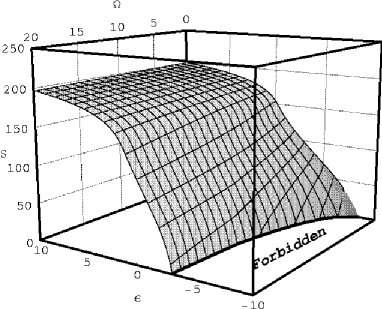
FIG. 2.: Entropy surface $S\left(\epsilon,\Omega\right)$, the mesh lines are at constant $\epsilon$ or constant $\Omega$. The thick line is close to the pojection of the $T=0$ ($S\to-\infty$) isotherm. A convex intruder at constant $\Omega$ and for a certain energy range (e.g. $-2<\epsilon<0$ for $\Omega=20$) can be seen for all $\Omega$. $S$ is not defined in the forbidden region; there the remaining energy $\epsilon_{r}$ is negative for all ${\bf q}\in v_{c}$.

Figure 2 shows the entropy surface $S$ as a function of $\epsilon$ and $\Omega$. The ground state energy $\epsilon_{g}(\Omega)$ (thick line in Fig. 2) increases with $\Omega$; $\epsilon_{g}$ classically corresponds to $\epsilon_{r}=0$ implying $S=-\infty$. For all $\Omega$, $\epsilon_{g}(\Omega)$ is a concave function of $\Omega$, i.e. $\frac{\partial^{2}\epsilon_{g}}{\partial\Omega^{2}}\leq 0$; at high $\Omega$ ($\Omega\gtrsim 12$) it is almost linear $\frac{\partial^{2}\epsilon_{g}}{\partial\Omega^{2}}\to 0^{-}$. These properties show that the set $\{\epsilon,\Omega\}$ over which $S$ is defined is not convex [49], and in Sec. III D we discuss some consequences resulting from a non–convex domain of definition.

At fixed $\Omega$, $S(\epsilon)$ is not concave for all $\epsilon$ but shows for some energy interval a convex intruder which signals a first order phase transition with negative specific heat $\left(\frac{\partial\beta}{\partial\epsilon}<0\right)$[33]. This can be better viewed by plotting $\beta(\epsilon,\Omega)=\frac{\partial S}{\partial\epsilon}$ (Fig. 3). Here the counter part of the entropy–intruder is a region of multiple valued $\epsilon(\beta)$, this is the case for $\beta$ between 15 and 20.

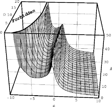
FIG. 3.: Inverse temperature $\beta(\epsilon,\Omega)$ surface. The mesh lines are at constant $\epsilon$ or constant $\Omega$. The intruder in $S$ at fixed $\Omega$ corresponds here to a multiple energy value for a given $\beta$ and $\Omega$, e.g. $\beta(\epsilon,\Omega=0)=20$ has three solutions $\epsilon_{1}\approx 0$, $\epsilon_{2}\approx-1$ and $\epsilon_{3}\approx-6$. The thick line is close to the projection of the $\beta=\infty$ isotherm; $\beta$ is not defined in the forbidden region.

The latent heat at fixed $\Omega$, $q_{\epsilon}(\Omega)$ decreases for $0\leq\Omega\lesssim 12$ and is a constant for $\Omega>12$. There is no critical value of $\Omega$, $\Omega_{c}$ above which $S(\epsilon)$ is concave for all $\epsilon$, i.e. there is a first order phase transition of all values of $\Omega$. In another model for a self–gravitating system such a $\Omega_{c}$ was reported [25], but not in the one presented in [14].

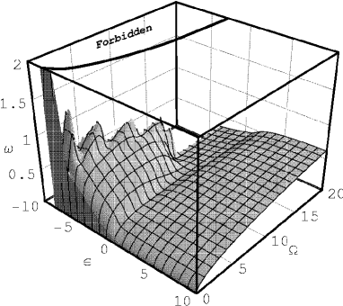
FIG. 4.: Microcanonical angular velocity $\omega\left(\epsilon,\Omega\right)$ surface. The mesh lines are at constant $\epsilon$ or constant $\Omega$. $\omega$ is not defined in the forbidden region. At high energy $\omega\propto\sqrt{\Omega}$; Near the ground states $\omega$ shows a richer non–monotonic behavior with peaks and troughs for small $\Omega$ and has a nearly constant value for large $\Omega$ (see text).

On Fig. 4 we have plotted the microcanonical angular velocity $\omega$ as a function of $\Omega$ and $\epsilon$. As a direct consequence of Eq. (9) $\omega$ tends to zero with $\Omega$, and at high energy $\omega$ is proportional to $\sqrt{\Omega}$ ($\propto L$). For low energies and $\Omega<12$, $\omega$ exhibits some structures with peaks and troughs, in another words at fixed $\epsilon$, $\omega$ is not necessarily an increasing function of $\Omega$. At high $\Omega$ ($\Omega>12$) and near the ground states $\omega$ is almost a constant. All these structures can be understood in terms of mass distributions which influence $\omega$ through $I$ (see Sec. III B).

B Mass distribution

In order to understand the origin of the structures seen in the different microcanonical quantities ($S$, $\beta$, $\omega$, $\ldots$) we have to have a closer look at the spatial configurations, i.e. at the mass distributions. One observable we have studied is the mass density $\rho$ (see Eq. 29 and 30). As the Hamiltonian of the system is rotationally invariant, the mean value of $\rho$ can only be a function of $r$, the distance from the center of coordinates, although other observables might show a breaking of the rotational symmetry (see below).

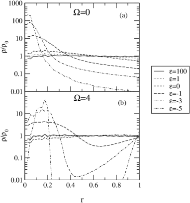
FIG. 5.: Density as a function of the distance from the center $r$ at different values of energy $\epsilon$ and angular velocity $\Omega$ (arbitrary units). At high energy and for all $\Omega$ the density is flat; the system is in the homogeneous gas phase. Near the ground state the density shows one peak for $\Omega=0$ (a) and two peaks for $\Omega>0$ (b), which correspond respectively to a one cluster and to a two clusters phase surrounded by some gas (see text).

On Fig. 5 $\rho$ is plotted for different energies and for $\Omega=0$ and $\Omega=4$. For $\Omega=0$ (Fig. 5.a) we recover the classical case (when $E$ is the only fixed parameter); at high energy the system is in a homogeneous gas phase (flat $\rho$), when the energy decreases the system undergoes a phase transition and eventually ends up in a collapse phase where a majority of particles are in a cluster near the center of coordinates ($\rho$ peaked at $r=0$). For $\Omega\neq 0$ (Fig. 5.b) the situation is (a little bit) different. At high energy we recover the homogeneous gas phase. But at low energy the system cannot collapse entirely at the center of mass. This is due to the rotational energy $\epsilon_{rot}=\frac{\Omega}{I}$ in Eq. (6); if the system contracts at the center the inertial momentum $I$ will tend to zero and therefore $\epsilon_{rot}$ will diverge leading to a negative remaining energy $\epsilon_{r}$. So depending on the value of $\Omega$ the main cluster will eject a certain amount of particles in order to increase $I$. Near the ground state these “free” particles will eventually collapse to form a second cluster in order to decrease the potential energy $\phi$. Due to the conservation of the center of mass, the position of the biggest cluster will be shifted from the center by a certain amount (see Fig. 5.b at $\epsilon=-5$). At low $\Omega$ one particle will be ejected, with increasing $\Omega$ the number of ejected particles raises and this process stops when two equal–size clusters are formed. This explains the discreteness of the peaks in $\omega$ (Fig. 4), the increase of the ground state energy $\epsilon_{g}(\Omega)$; because the potential energy of a single cluster of size $N$ is smaller than the one of two well separated clusters. At high $\Omega\gtrsim 12$ the system undergoes a phase transition from a gas phase to a collapse phase with two equal size clusters close to the boundary. From one value of $\Omega=\Omega_{1}>12$ to another one $\Omega_{2}>\Omega_{1}$ the whole entropy curve at fixed angular momentum is simply shifted along the energy axis, i.e. $S\left(\epsilon,\Omega_{1}\right)\approx S\left(\epsilon+\frac{\Omega_{2}-\Omega_{1}}{N},\Omega_{2}\right)$. So the ground state energy $\epsilon_{g}(\Omega)$ at high $\Omega$ is almost on a line of equation $\epsilon_{g}+\frac{\Omega}{N}+\phi_{g}\approx 0$, where $\frac{\Omega}{N}$ and $\phi_{g}$ are the rotational energy and the potential energy of 2 clusters of size $N/2$ at radius $r=1$ respectively. This monotonic behavior has already be mentioned for all the thermodynamical variables $S$ (Fig. 2), $\beta$ (Fig. 3), $\omega$ (Fig. 4)…

As already mentioned $\rho$ is only a function of $r$ and it can not be used to infer the angular distribution of the particles, i.e. there is not enough information to say if a peak in $\rho$ at $r_{0}\neq 0$ corresponds to one or many clusters or to a uniform distribution of the particles (ring) lying on a circle of radius $r_{0}$. However at least at very low energy a many clusters (more than two) configuration is very unlikely and will not contribute to the average values for reasons linked to the weight $W(\mbox{\boldmath$r$})=\frac{1}{\sqrt{I}}\epsilon_{r}^{N-5/2}$. For simplicity let us assume that there is only one strong peak in $\rho$ at $r=r_{0}\neq 0$. Since the center of mass is fixed this can not be the signature of a 1–cluster system. At least 2–clusters lying on a circle of radius $r_{0}$ are needed. All these n–clusters systems have the same rotational energy $\frac{\Omega}{I}=\frac{\Omega}{Nr_{0}^{2}}$, but their corresponding potential energy $\phi_{n}$ will differ. For example, with $\sigma=0.05$, $r_{0}=0.5$ and $N=24$ the ratio of potential energy is $\frac{\phi_{2}}{\phi_{3}}\simeq 1.7$. So at low energy, the remaining energy $\epsilon_{r}$ corresponding to a 2–clusters system will be much larger than the 3–clusters’ one, leading to a huge difference in the weight $W(\mbox{\boldmath$r$})$. So at low energy and for $\Omega\neq 0$ the 2–clusters case is dominant. At higher energies, the term $Bg(I,\phi)$ in Eq. (25) can compensate the difference in the weight $W(\mbox{\boldmath$r$})$ and allow many clusters configurations and eventually at high energy a complete random configuration on the ring of radius $r_{0}$ will dominate the average mass distribution.

We can check this argument by studying another observable, for example the normalized distance distribution $P(d)$, i.e. the density of probability that the distance between two given particles is $d$. To probe the information given by $P(d)$ we have estimated it for four simple mass distributions: (a) 2–clusters, (b) 3–clusters, (c) ring, (d) uniform random distribution. For (a), (b) and (c) the particle were put on a circle of radius $r_{0}=0.5$, and then randomly shifted several times (in order to give a spatial extension to these idealized initial configurations); finally the $\frac{N(N-1)}{2}$ distances are recorded for all realizations and averaged. Figure 6 shows the average of $P(d)$ over 1000 realizations. Note that the density distribution $\rho(r)$ is by construction exactly the same for the three first cases, i.e. strongly peaked at $r_{0}$ with a width of about $0.5$. The latter value depends on the shift one applies on the initial idealized spatial configurations.

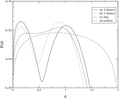
FIG. 6.: Average of $P(d)$ the distance distribution for different simulated spatial configurations. See text.

As one can see on Fig. 6, although the density distribution is the same for (a), (b) and (c), $P(d)$ gives some new insight on the mass distribution:

• There are two peaks, one at small $d$ which corresponds to a clusterisation and another one at $r=1=2r_{0}$; this is exactly the distance between the two clusters (more precisely between their center of mass). The area under the small $d$ peak is similar to the one under the large $d$ peak, indeed the number of short distance pairs and the number of pairs with $d\simeq 1$ are both about $\frac{N^{2}}{4}$. Moreover the widths of the first and second peaks are (as expected) $\sim 0.5$ and $\sim 1=2*0.5$ respectively.

• There are again two peaks one at small $d$ and another at $d\simeq 0.8<1$ and their respective widths are similar to the ones in (a). The large $d$ is compatible with the length of one side of the equilateral triangle on top of which the 3–clusters mass distribution has been built. This time the area under the large $d$ peak is larger than the one under the short $d$ peak, since the number of short distance pairs is about $\frac{N^{2}}{6}$ whereas the number of pairs with $d\simeq 0.8$ is $\frac{N^{2}}{3}$.

• In the ring a trace of the two peaks still exists but they are not well separated because a lot of intermediate distances are compatible with this model.

• When the particles are uniformly distributed $P(d)$ is a binomial–like distribution.

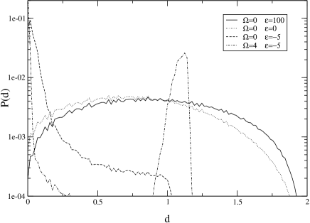
FIG. 7.: Distance distribution $P(d)$ for the gravitational case for different values of $(\epsilon,\Omega)$. At high energy $P(d)$ corresponds to a random distribution (see Fig. 6). For $\Omega=0$ and at low energy, $P(d)$ has one peak at $d\approx 0$; almost all particles are very close from each other, and there is a single cluster collapse phase. For $\Omega\neq 0$ there are two peaks at low energy: one at very small $d$ which is a sign of clusterisation and another peak at large $d$ which signals multiple clusterisations; in fact there are two clusters (see text).

We have also estimated $P(d)$ for our gravitational system, as shown on Fig 7. At high energy, $P(d)$ corresponds to the randomly distributed case (see Fig. 6). At low energy with $\Omega=0$, $P(d)$ has only one peak at $d=0$, this corresponds clearly to a single cluster case surrounded by some gas. For $\Omega\neq 0$ and at low energy (in Fig. 7 $\epsilon=-5$ and $\Omega=4$), there are two well separated peaks, one at small $d_{0}=0$ and the other at $d_{1}\simeq 1.1$. The peaks imply the presence of at least two clusters, however the fact that the widths of the peaks are small excludes a large number of clusters and even more the ring case (see Fig. 6). Now we can combine these informations with the ones obtained by studying $\rho(r)$ (see Fig. 5). For $\epsilon=-5$ and $\Omega=4$, $\rho$ has two peaks at $r_{1}\simeq 0.15$ and $r_{2}\simeq 1$. All in all, this means that there are, in the mean, two clusters rotating around the center of mass. The distance between these clusters is $r_{1}+r_{2}\simeq 1.15\simeq d_{1}$. Their mass ratio is $\frac{m_{2}}{m_{1}}=\frac{r_{1}}{r_{2}}\simeq 0.15$. Since we know the total mass $m_{1}+m_{2}=20$ we get $m_{1}\simeq 17$ and $m_{2}\simeq 3$.

The distance distribution can be of great help to identify the mass distributions at low energies. However at the transition regions since there is a superposition of different types of mass distributions the knowledge $\rho$ and $P(d)$ is not sufficient and therefore of no help if we want to study for example the “fractality” of the mass distribution as it has been discussed in other self–gravitating systems  [50, 51, 52] (not mentioning the fact that the actual number of particles in the presented numerical applications is too small), and further work is needed to get a more detailed picture.

At very low energy, near the ground state at least one of the clusters (the smallest) is very close to the boundary. There the assumption of a small evaporation rate made in Sec. I does not hold.

C Phase diagram

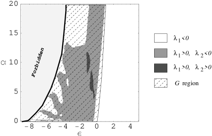
FIG. 8.: ${\rm sign}\left(\lambda_{1}(\epsilon,\Omega)\right)$ as defined in Sec. II B. The white regions correspond to $\lambda_{1}<0$ and therefore to a positive determinant $D_{S}=\lambda_{1}\lambda_{2}>0$ of the entropy curvature, these are pure phase regions. The gray region corresponds to $\lambda_{1}>0$ and $D_{S}<0$ and the dark gray ones also to $\lambda_{1}>0$ but $D_{S}>0$; $\lambda_{1}>0$ defines first order phase transition regions (see text). Points in $G$ correspond to local maxima (minima) in Eq. (31) if $\lambda_{1}<0$ ($\lambda_{1}>0$) but not to global maxima (minima); points outside $G$ correspond to global maxima in Eq. (31). There is a one–to–one mapping between the microcanonical ensemble and the GBE only in the white region (see text). $S$ is not defined in the forbidden region, here in light gray. Note that (a) the points at $\Omega=0$ and low energies $\epsilon<-7$ are not included in $G$, (b) the high energy limit of $G$ is only known approximatively.

On Fig. 8 we have plotted ${\rm sign}\left(\lambda_{1}(\epsilon,\Omega)\right)$ as defined in Sec. II B. This plot can be taken as the phase diagram of the self–gravitating system at fixed $\epsilon$ and $\Omega$. The white regions correspond to pure phases ($\lambda_{1}<0$ ). At high energy there is a homogeneous gas phase and at low energy there are several pure collapse phases with one ($\Omega=0$) or two ($\Omega\neq 0$) clusters. The different 2–clusters phases are characterized by the relative size of their clusters (see Sec. III B). These regions are separated by first order phase transition regions where $\lambda_{1}>0$ (gray in Fig. 8). There are even two regions (dark gray) where the entropy $S$ is a convex function of $\epsilon$ and $\omega$; i.e. all the eigenvalues of $J_{S}$ are positive ($\lambda_{1}>0$ and $D_{S}>0$). These two regions are quite stable with respect to the number of particles (at least for $N<50$). Their surface increase slightly with the number of particles $N$. The orientation of ${\bf v}_{1}$ the eigenvector associated with $\lambda_{1}$ (defined as the largest eigenvalue of $J_{S}$) is not yet known in detail for all $(\epsilon,\Omega)$; however we can already state that at “high” energy ${\bf v}_{1}$ is almost parallel to the energy axes (phase transition in the $\epsilon$ direction) and should be parallel to the ground state at very low energy. The overall structure of the collapse phases matches the one of the angular velocity $\omega$ (see Fig. 4): roughly, the peaks in $\omega$ correspond to pure phases while the valleys between these peaks belong to the first order phase transition region. Due to a lack of precision we are yet unable to ensure that the two isolated pure phases at $\epsilon\approx-4$, $\Omega\approx 1$ and $\Omega\approx 7$ are really isolated and not linked to a pure phase at lower energies.

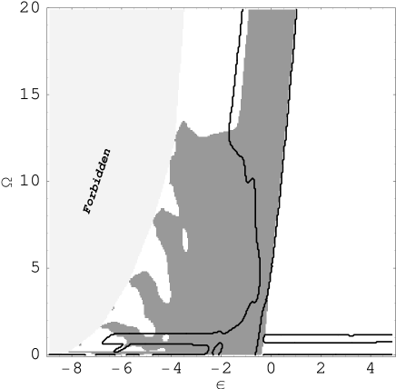
FIG. 9.: Locus of second order phase transitions (see text).

As already mentioned, unlike in the model presented by Laliena in [25] there is no critical angular momentum $L_{c}$ above which the first order phase transition vanishes giving rise to a second order phase transition at $L_{c}$. Nevertheless this does not exclude second order phase transition (critical point) at all. They are defined in the microcanonical ensemble by: (i) $\lambda_{1}=0$; (ii) $\nabla\lambda_{1}\cdot{\bf v}_{1}=0$ (see Sec II B). On Fig. 9 (just like on Fig. 8) regions where $\lambda_{1}<0$ ($>0$) are in white (gray). The condition (i) is simply achieved at the boarder between the gray and the white regions. The thick lines on Fig. 9 correspond to condition (ii). Second order phase transition are located at the crossing points points of the thick lines and the boarders. One immediately sees that there are several critical points. However there are not all of (astro–)physical interest since most of them are close to the ground states line or at very high angular momentum where the small evaporation rate assumption is not valid. Nevertheless there are two points one at $(\epsilon,\Omega)\approx(-0.5,1)$ and another one at $(\epsilon,\Omega)\approx(-0,4)$ where this assumption is valid and therefore their deserve further investigations and especially regarding their corresponding mass distributions.

D Loss of information in the $(\beta,\beta\gamma)$ ensemble (GBE)

In a recent paper Klinko and Miller have studied another model for rotating self–gravitating systems [14]. They introduced the canonical analogous of the $(\epsilon,\Omega)$ ensemble namely the $(\beta,\gamma\beta)$ ensemble (GBE), see Eq. (7) and (10). Once one defines the generalized microcanonical ensemble (ME), it is straightforward to introduce and study the system in its conjugate ensemble, the generalized canonical ensemble (CE). Note that “generalized” means in CE “as a function of all the intensive variables” and, in ME “as a function of all extensive parameters”. There are mainly two reasons invoked to study a system in CE instead of in ME

1. Performing the computations in CE are in most cases much easier than in ME. Here CE can be seen as a trick [53]. However there is a priori no reason for the results to be equivalent. Indeed the strict equivalence of the ensemble is only achieved at the thermodynamical limit except in the first order phase transition regions [33, 32, 42]. In a weaker sense, needed for Small systems, ME and CE can only be equivalent when $\lambda_{1}(X)<0$ and far from any first order phase transition regions (see below). Moreover recent progress in computer performance enables one to perform now numerical experiments within the ME for increasingly complex systems.

2. The studied system is not isolated but is in contact with a “heat bath” and exchange amounts of $X$ with it. Then, obviously ME does not provide a suitable description, and CE might be eligible. Here CE describes a different physical system than the one in ME. At the thermodynamical limit (if it exists) the ensembles are again equivalent except at first order phase transitions. However, the CE description is valid only if the Hamiltonian of interaction ${\cal H}_{int}$ is small comparing to the ones of the system ${\cal H}_{sys}$ and the heat bath ${\cal H}_{hb}$. This condition is usually fulfilled at the thermodynamical limit (if it exists), but for Small ones ${\cal H}_{int}$ can hardly be small at least comparing to ${\cal H}_{sys}$ and this can lead to dramatic effects [54, 55]. In this case a better description would be the ME of the system, its “heat bath” and their interactions.

For now on we consider in this paper the cases when CE is used as a mathematical trick, and we focus and the amount of information lost from ME to CE.

The link between ME and CE is given by Laplace transform (using the notations introduced in Sec. II B)

$${\cal Z}(x)=\int_{0}^{\infty}dX\>e^{-X\cdot x+S(X)},$$ (31)

where ${\cal Z}$ is the partition sum of the CE; $x=\{x^{1},\ldots,x^{{\cal N}}\}$ are the intensive variables associated with $X$ and defined by

$$x^{i}\equiv\frac{\partial S}{\partial X^{i}},$$ (32)

for $i=1,\ldots,{\cal N}$. The ME at $X_{0}$ is equivalent to the CE at $x_{0}=x(X_{0})$ if the integrand in Eq. (31) $e^{f(X,x_{0})}$, and therefore $f(X,x_{0})=-X\cdot x_{0}+S(X)$ has a global maximum at $X_{0}$. This condition is violated when $\lambda_{1}(X_{0})>0$ (this is the basic idea behind the definition of phase transitions in Small systems, see [32]). So in practice all informations contained in points where $\lambda_{1}>0$ are lost after the Laplace transform (31) in CE.

Now we are left with the points $X_{0}$ characterized by $\lambda_{1}(X_{0})<0$; this relation implies only that $f(X,x_{0})$ has a local maximum at $X_{0}$ but not that it is a global one; $\lambda_{1}<0$ is a necessary but not sufficient condition. In Fig. 10 we have illustrated this point with a trivial one–dimensional example; all the points below the Maxwell line do not correspond to global maxima and their information content is smeared out and, in practice, lost in CE.

FIG. 10.: Schematic entropy curve $S$ as a function of one extensive parameter $X$ (solid line) and the Maxwell line (dashed line). $A$ and $D$ are the end points of the Maxwell construction. At $B$ and $C$ the largest curvature vanishes, i.e. $\lambda_{1}=0$. All the points below the Maxwell line do not not correspond to a global maximum in the Laplace transform Eq. (31). This includes points where $\lambda_{1}=\frac{\partial^{2}S}{\partial X^{2}}>0$, but also points where the entropy is concave, for $X\in[X_{A},X_{B}]$ and $X\in[X_{A},X_{B}]$, $\lambda_{1}(X)<0$.

From the last remark we see that a way to check if a point corresponds to a global maximum in Eq. (31) is to study what would be a generalization of the Maxwell line in ${\cal N}>1$ dimensions. Work is in progress in this direction and the results will be presented elsewhere, but we can already state that this task is, to some extent, similar to the one of building the convex hull of a set of points in ${\cal N}$ dimensions, or more specifically the convex hull of the entropy $S$.

However, if one needs qualitative results, in two dimensions the task can be rather easily solved in another way. Let us define $p(X,X_{0})$ the tangent plane to $S(X)$ at $X_{0}$; its equation is $p(X,X_{0})=-X\cdot x_{0}+S(X_{0})+X_{0}\cdot x_{0}$. If $f(X,x_{0})$ has a global maximum at $X_{0}$ then

$$p(X,X_{0})>S(X)$$ (33)

for all $X\neq X_{0}$ and $p(X_{0},X_{0})=S(X_{0})$ by definition.

In the case of the gravitational model presented here $X=\{\epsilon,\Omega\}$ and $x=\{\beta,\gamma\beta\}$. Now if one inspects the entropy surface $S(X)$ (see Fig. 2) it is clear that condition (33) is not satisfied for all the points in the region filled with dashed lines ($G$) in Fig. 8. This is due to the concavity of the energy ground state $\epsilon_{g}(\Omega)$ (see Sec. III A). $G$ includes all the two–clusters collapsed phases, the first and second order phase transitions (except for $\omega=\Omega=\gamma=0$). All the information contained in $G$ is smeared out through the Laplace transform (31) in GBE and, in practice, lost.

The fact that GBE misses all the two–clusters collapse phases would be already enough to disqualify it as being a good approximation (mathematical trick) of the ME. But, furthermore, if one studies more carefully $f(X,x_{0})$, $X_{0}\in G$; one will notice that (a) there is one local maximum at $\Omega=0$ and (b) there is no maximum for high $\Omega$: in the direction of increasing $\Omega$ at low energy, $f(X,x_{0})$ is a never ending increasing function, i.e. $f(X,x_{0})$ has no global maximum for $X\in G$ (see Fig. 11). Therefore the integral in Eq. (31) diverges for all $x_{0}$, $X_{0}\in G$. In other words the GBE, in our model, is not defined for high $\beta$ and $\gamma\neq 0$ ($\omega\neq 0$).

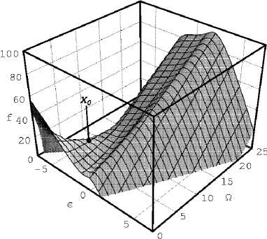
FIG. 11.: $f(\epsilon,\Omega,\beta_{0},\gamma_{0})=-\epsilon\beta_{0}-\Omega\beta_{0}\gamma_{0}+S(\epsilon,\Omega)-K$ as a function of $\epsilon$ and $\Omega$, where $K$ is an arbitrary constant; $\beta_{0}=\beta(\epsilon_{0},\Omega_{0})$; $\Omega_{0}=\Omega(\epsilon_{0},\Omega_{0})$; $X_{0}=(\epsilon_{0},\Omega_{0})=(-3,5)\Rightarrow(\Omega_{0},\gamma_{0})\approx(27.9,-0.196)$. The mesh lines are at constant $\epsilon$ or constant $\Omega$. As expected $f$ has a saddle point at $X_{0}\approx(\beta_{0},\gamma_{0})$ since $m(X_{0})>0$ and $D_{S}(X_{0})<0$ (see text and Fig. 8). $f$ has a global maximum at $\Omega=0$ and $\epsilon\approx-7$, but one sees that it is an monotonically increasing function for increasing $\Omega$ and $\epsilon(\Omega)\approx\epsilon_{g}(\Omega)+2$. Therefore the integral in Eq. (31) diverges and the $(\beta,\gamma\beta)$ ensemble is not defined for $(\beta_{0},\gamma_{0})$.

This example shows how dramatic can be the information loss if one studies an isolated system in the CE.

IV Summary and discussion

A Summary

The aim of this paper is to present the results of a study of a self–gravitating system of $N$ classical particles on a disk of radius $R$ for which two extensive variables, namely total energy $E$ and total angular momentum $L$ are fixed. The microcanonical entropy $S$ can be written as the logarithm of an integral over the spatial configurations (3) and (6). The conservation of $L$ implies that the mean value of the linear momentum $p$ of a particle at a radial distance $r$ is proportional to $L$ and $r$ (14); in the mean the system rotates like a solid body, i.e. the mean angular velocity of a particle does not depend on its position (19). The dispersion of $p$ is broader than the one it had if $L$ would not be conserved and depends on the radial position (21). In order to integrate $e^{S}$ we write it as the folding product of a “background” function $Bg$ and the weight associated with the remaining energy (25). Once a numerical estimate of $Bg$ is obtained, $S$ and its derivatives, such as the inverse temperature $\beta$, can be computed. The entropy surface shows an intruder in the energy direction which signals a first order phase transition with negative specific heat (Fig. 2 and Fig. 3). Contrary to another model [25] there is no critical value of $L$ above which this transition is no longer present, nevertheless there are several points of the parametric space $\left(E,L\right)$ . At high energy the angular velocity $\omega$ is a simple increasing function of $L$ (Eq. (9) and Fig. 4), but at low energy, near the ground states the relation between $L$ and $\omega$ becomes non–trivial. All these peculiarities can be understood if we study the mass distribution. We use two observables: the density of mass $\rho$ as a function of the radial distance; and $P(d)$ the density probability that the distance between two particles is $d$. At fixed $L$ and at high energy the particles are randomly distributed over the disk (gas phase); if the energy decreases, at some threshold the system undergoes a phase transition of first order to a collapse phase. If $L=0$ there is a single cluster at the center of mass, if $L\neq 0$ then there are two clusters rotating around the center of mass. Their relative mass $\frac{m_{1}}{m_{2}}$ with $m_{1}>m_{2}$ is very large for low $L$, it decreases as $L$ raises and eventually becomes 1 for $L$ larger than a certain threshold. Clearly these two clusters phases were not reported in previous work because of the usual a priori assumption of rotaional symmetry.

Phase transitions (and phases) can be defined unambiguously in the microcanonical ensemble as a function of the local topology of $S$. If all eigenvalues of $J_{S}$, the Jacobian of $S$ are negative then the system is in a pure phase. If (at least) one eigenvalue is positive, say $\lambda_{1}$, then there is a first order phase transition in the direction of ${\bf v}_{1}$, the eigenvector associated with $\lambda_{1}$. A critical behavior occurs when one (or many) eigenvalue vanishes on at least a second order region (if $\lambda_{i}=0$, $\nabla_{{\bf v}_{i}}\lambda_{i}=0$). Note that one can find positive, negative and zero eigenvalues at the same point in the parameter space. Using these criteria, we can draw a phase diagram of the gravitational system (Fig. 8) at fixed $E$ and $L$: at high energy there is a pure gas phase; at low energy there are several pure collapse phases, there is one cluster at $L=0$ and there are two clusters for $L\neq 0$; these phases are separated by first order phase transition regions. There are also several second order phase transitions; two of them are located at relativley high energies ($E\approx 0$) and therefore may be of astrophysical importance.

Studying an isolated system using the canonical ensemble (CE) can be very misleading, since there is a massive loss of information from the correct microcanonical ensemble (ME) description to the CE’s one (if there are phase transitions in ME). In fact for the gravitational model, CE cannot be sensitive to the two clusters phases and all the phase transitions and it is not defined for some values of the intensive parameters that exist in ME (see Sec. III D).

B Discussion

Of course we have just presented an equilibirum statistical model that may help to understand the physics of globular clusters or collapsing molecular clouds and the results should be interpreted with caution especial in the case of star formation. A lot of “ingredients” are missing in order to have a complete picture of the formation of multiple stars systems and planetary systems, for instance the magnetic field [56, 57], or the presence of vortices [58].

Phases and phase transitions can be well defined in the microcanonical ensemble (ME) without invoking the thermodynamical limit by probing the curvature of the entropy surface. There still exists open problems. One of them is the scaling of a first order transition: in Fig. 10 in a canonical sense the phase transition occurs from $X_{A}$ to $X_{D}$ (if $X$ is the energy $E$ then $X_{D}-X_{A}$ is the transition latent heat), but for if one uses the ME definition the transition occurs only from $X_{B}$ to $X_{C}$. At the thermodynamical limit, if it exists, such discrepancy should disappear. In another context (a model of a first order liquid gas transition of finite–size Sodium clusters) we could show that $\frac{X_{C}-X_{B}}{X_{D}-X_{A}}\to 1$ when the system size goes to infinity.

The ME definition of phase transitions offers a richer view of physical systems and phase transitions. Again on Fig. 10, CE is not sensitive to everything that could happen under the Maxwell line: there is always one transition. On the contrary, in ME there could be many phase transitions between $X_{A}$ and $X_{D}$. For example if there is a small positive curvature bump between $X_{B}$ and $X_{C}$ there would be two transitions in the microcanonical sense but still one in the canonical sense.

A

Let us compute $\langle\mbox{\boldmath$p$}_{k}\rangle_{\mbox{\boldmath$q$}_{k}}$ the average momentum of particle $k$ at fixed position (for simplicity we will set $k=1$). The $\alpha$–component of $\langle\mbox{\boldmath$p$}_{1}\rangle_{\mbox{\boldmath$q$}_{1}}$ is

$$\langle p_{1}^{\alpha}\rangle_{\mbox{\boldmath$q$}_{1}} = \frac{\int\left(\prod_{i}d\mbox{\boldmath$p$}_{i}\prod_{i=2}^{N}d\mbox{\boldmath$q$}_{i}\right)p_{1}^{\alpha}\delta\left(E-{\cal H}\right)\delta^{2}\left(\sum_{i}\mbox{\boldmath$p$}_{i}\right)\delta\left(\sum_{i}\mbox{\boldmath$q$}_{i}\times\mbox{\boldmath$p$}_{i}-L\right)\delta^{2}\left(\sum_{i}\mbox{\boldmath$q$}_{i}\right)}{\int\left(\prod_{i}d\mbox{\boldmath$p$}_{i}\prod_{i=2}^{N}d\mbox{\boldmath$q$}_{i}\right)\delta\left(E-{\cal H}\right)\delta^{2}\left(\sum_{i}\mbox{\boldmath$p$}_{i}\right)\delta\left(\sum_{i}\mbox{\boldmath$q$}_{i}\times\mbox{\boldmath$p$}_{i}-L\right)\delta^{2}\left(\sum_{i}\mbox{\boldmath$q$}_{i}\right)}$$ (A1)

$$= \frac{\int\left(\prod_{i=2}^{N}d\mbox{\boldmath$q$}_{i}\right){\cal P}_{1}^{\alpha}\delta^{2}\left(\sum_{i}\mbox{\boldmath$q$}_{i}\right)}{\int\left(\prod_{i=2}^{N}d\mbox{\boldmath$q$}_{i}\right)W({\bf r})\delta^{2}\left(\sum_{i}\mbox{\boldmath$q$}_{i}\right)},$$ (A2)

where ${\cal P}_{1}^{\alpha}=\int\left(\prod_{i}d\mbox{\boldmath$p$}_{i}\right)p_{1}^{\alpha}\delta\left(E-{\cal H}\right)\delta^{2}\left(\sum_{i}\mbox{\boldmath$p$}_{i}\right)\delta\left(\sum_{i}\mbox{\boldmath$q$}_{i}\times\mbox{\boldmath$p$}_{i}-L\right)$, and $W({\bf r})$ is the microcanonical weight at fixed spatial configuration ${\bf r}$, its value is $W(E,L,{\bf r})={\cal C}\frac{1}{\sqrt{I}}E_{r}^{N-5/2}$ (see (6)). The outline of the derivation of ${\cal P}_{1}^{\alpha}$ is the same as in [25] for $W$, and we get after some algebra

$${\cal P}_{1}^{\alpha}={\cal C}Lm_{1}I^{-3/2}\sum_{\delta=1}^{2}r_{1}^{\delta}\epsilon_{\delta\alpha}\>E_{r}^{N-5/2},$$ (A3)

where ${\bf\epsilon}$ is the antisymmetric tensor of rank 2. Using (A3) in (A2) we get finally

$$\langle p_{1}^{\alpha}\rangle_{\mbox{\boldmath$q$}_{1}} = \frac{\int\left(\prod_{i=2}^{N}d\mbox{\boldmath$q$}_{i}\right){\cal C}Lm_{1}I^{-3/2}\sum_{\delta=1}^{2}r_{1}^{\delta}\epsilon_{\delta\alpha}\>E_{r}^{N-5/2}\delta^{2}\left(\sum_{i}\mbox{\boldmath$q$}_{i}\right)}{\int\left(\prod_{i=2}^{N}d\mbox{\boldmath$q$}_{i}\right)I^{-1/2}\sum_{\delta=1}^{2}r_{1}^{\delta}\epsilon_{\delta\alpha}\>E_{r}^{N-5/2}\delta^{2}\left(\sum_{i}\mbox{\boldmath$q$}_{i}\right)}$$ (A4)

$$= Lm_{1}\langle I^{-1}\rangle_{{\bf r}_{k}}\sum_{\delta}r_{1}^{\delta}\epsilon_{\delta\alpha}.$$ (A5)

Finally

$$\langle\mbox{\boldmath$p$}_{1}\rangle_{\mbox{\boldmath$r$}_{1}}=Lm_{1}\langle I^{-1}\rangle_{{\bf r}_{k}}\sum_{\delta,\alpha}r_{1}^{\delta}\epsilon_{\delta\alpha}{\bf e_{\alpha}},$$ (A6)

where ${\bf e_{\alpha}}$ is the $\alpha$–component unit vector.

$\langle\mbox{\boldmath$p$}_{k}^{2}\rangle_{\mbox{\boldmath$q$}_{k}}$ can be derived in a similar way, and we get

$$\langle\mbox{\boldmath$p$}_{k}^{2}\rangle_{\mbox{\boldmath$q$}_{k}} = \frac{2m_{k}}{(N-5/2)\langle Er^{-1}\rangle_{\mbox{\boldmath$q$}_{k}}}\left(1-\frac{m_{k}}{M}\right)$$ (A8)

$$-\frac{m_{k}I_{k}}{I(N-5/2)\langle Er^{-1}\rangle_{\mbox{\boldmath$q$}_{k}}}+I_{k}L^{2}m_{k}\langle I^{-2}\rangle_{\mbox{\boldmath$q$}_{k}}.$$

REFERENCES

- [1] V. Antonov, Vestn, Leningr. Gros. Univ. 7, 135 (1962).
- [2] T. Padmanabhan, Physics Report 188, 285 (1990).
- [3] D. Lynden–Bell, Mon. Not. R. Astron. Soc. 136, 101+ (1967).
- [4] D. Lynden–Bell and R. Wood, Mon. Not. R. Astron. Soc. 138, 495+ (1968).
- [5] P. Hertel and W. Thirring, Annals of Physics 63, 520 (1971).
- [6] W. Thirring, Z. Phys. 235, 339 (1970).
- [7] W. C. Saslaw, Gravitational physics of stellar and galactic systems (Cambridge University Press, Cambridge, 1985).
- [8] G. B. Lima Neto, D. Gerbal, and I. Márquez, Mon. Not. R. Astron. Soc. 309, 481 (1999).
- [9] A. R. Lima, P. M. C. de Oliveira, and T. J. P. Penna, J. Stat. Phys. 99, 691 (2000).
- [10] J. Binney and S. Tremaine, Galactic dynamics (Princeton series in astrophysics, Princeton, NJ, 1987).
- [11] C. Lagoute and P.-Y. Longaretti, Astron. Astrophys. 308, 441 (1996).
- [12] C. Lagoute and P.-Y. Longaretti, Astron. Astrophys. 308, 453 (1996).
- [13] G. Horwitz and J. Katz, Astron. J. 211, 226 (1977).
- [14] P. J. Klinko and B. N. Miller, Mean Field Theory of Spherical Gravitating Systems, e–print arXiv.org/cond-mat/0007065, 2000.
- [15] D. Lynden-Bell, Rotation, Statistical Dynamics and Kinematics of Globular Clusters, e–print arXiv.org/astro-ph/0007116, 2000.
- [16] F. Combes, in Chaotic Dynamics of Gravitational Systems, Les Arcs 2000, edited by C. Mechanics (1998).
- [17] H. J. de Vega, N. Sánchez, and F. Combes, Fractal Structures and Scaling Laws in the Universe: Statistical Mechanics of the Self–Gravitating Gas, Invited paper to the special issue of the ‘Journal of Chaos, Solitons and Fractals’: ‘Superstrings, M, F, S…theory’, M. S El Naschie and C. Castro, Editors.
- [18] M. R. Bate, Astron. J. Lett. 518, L95 (1998).
- [19] R. I. Klein, R. T. Fisher, C. F. McKee, and J. K. Truelove, in Proceedings of Numerical Astrophysics 1998 (1998).
- [20] R. S. Klessen and A. Burkert, in Riken Symposium on Supercomputing (1997).
- [21] A. Burkert and P. Bodenheimer, Mon. Not. R. Astron. Soc. 280, 1190 (1996).
- [22] A. P. Whitworth, N. F. A. S. Bhattal, and S. J. Watkins, Mon. Not. R. Astron. Soc. 283, 1061 (1996).
- [23] S. D. M. White, in Gravitational Dynamics, edited by E. T. R. Terlevich, O. Lahav (Cambridge Univ. Press, Cambridge, 1996).
- [24] D. M. Christodoulou and J. E. Tohline, Astron. J. 363, 197 (1990).
- [25] V. Laliena, Phys. Rev. E 59, 4786 (1999).
- [26] K. R. Yawn and B. N. Miller, Phys. Rev. E 56, 2429 (1997).
- [27] C. J. Reidl, Jr. and M. B. N., Phys. Rev. E 48, 4250 (1993).
- [28] J. Sommer-Larsen, H. Vedel, and U. Hellsten, Astron. J. 500, 610 (1997).
- [29] E. Follana and V. Laliena, Phys. Rev. E 61, 6270 (2000).
- [30] P.-H. Chavanis, Phys. Rev. E 58, R1199 (1998).
- [31] T. D. Lee and C. N. Yang, Phys. Rev. 87, 410 (1952).
- [32] D. H. E. Gross and E. Votyakov, Eur. Phys. J. B 15, 115 (2000).
- [33] D. H. E. Gross, Physics Report 279, 119 (1997).
- [34] H. C. Plummer, Mon. Not. R. Astron. Soc. 71, 460 (1911).
- [35] G. Yepes, in From quantum fluctuations to cosmological structures, Vol. 126 of ASP Conferences, edited by D. Valls-Gabaud, M. Hendry, P. Molaro, and K. Chamcham (Astronomical Society of the Pacific, Provo, Utah USA, 1997), p. 279.
- [36] F. Calvo and P. Labastie, Eur. Phys. J. D 3, 229 (1998).
- [37] B. Diu, C. Guthmann, D. Lederer, and B. Roulet, Physique Statistique (Hermann, 293 rue Lecourbe, 75015 Paris, France, 1989).
- [38] R. E. Kunz and R. Berry, Phys. Rev. E 49, 1895 (1994).
- [39] D. H. E. Gross and P. A. Hervieux, Z. Phys. D 33, 295 (1995).
- [40] H. A. Posch, H. Narnhofer, and W. Thirring, Phys. Rev. A 42, 1880 (1990).
- [41] D. H. E. Gross, M. E. Madjet, and O. Schapiro, Z.Phys.D 39, 75 (1997).
- [42] L. Landau and E. Lifchitz, in Physique statistique (Mir–Ellipses, Moskow, 1994), Chap. II.26.
- [43] A. Torcini and M. Antoni, Phys. Rev. E 59, 2746 (1999).
- [44] J. Lee, Phys. Rev. Lett. 71, 211 (1993).
- [45] B. A. Berg and U. Hansmann, Phys. Rev. B 47, 497 (1993).
- [46] A. M. Ferrenberg and R. H. Swendsen, Phys. Rev. Lett. 63, 1195 (1989).
- [47] G. R. Smith, Ph.D. thesis, University of Edinburgh, 1996.
- [48] O. Fliegans, Ph.D. thesis, Freie Universität Berlin, 2001.
- [49] A set of is said to be convex if for any couple of points and () of , the segment is in .
- [50] H. J. de Vega and N. Sánchez, Physics Letter B 490, 180 (2000).
- [51] Y. Sota, O. Iguchi, M. Morikawa, T. Tatekawa, and K. ichi Maeda, The Origin of Fractal Distribution in Self–Gravitating Virialized System and Self–Organized Criticality, e–print arXiv.org/astro-ph/0009412, 2000.
- [52] B. Semelin, Ph.D. thesis, Université Paris VI, 1999.
- [53] P. Ehrenfest and T. Ehrenfest, The Conceptual Foundation of the Statistical Approach in Mechanics (Cornell University Press, Ithaca NY, 1959), pp. 20–22.
- [54] K. Sato, K. Sekimoto, T. Hondou, and F. Takagi, Irreversibility resulting from contact with a heat bath caused by the finiteness of the system, e–print arXiv.org/cond-mat/0008393, 2000.
- [55] K. Sekimoto, F. Takagi, and T. Hondou, The Carnot Cycle for Small Systems: Irreversibility and the Cost of Operations, Phys. Rev. E 62, 7759 (2000), e–print arXiv.org/astro-ph/0003064.
- [56] A. Hujeirat, P. Myers, M. Camenzind, and A. Burkert, New Astronomy 4, 601 (2000).
- [57] D. Galli, F. H. Shu, G. Laughlin, and S. Lizano, in Stellar Clusters and Associations, Vol. 198 of ASP Conference Series, edited by T. Montmerle and P. André (ASP, Provo, Utah USA, 2000).
- [58] P.-H. Chavanis, Astron. Astrophys. 356, 1089 (2000).