Statistics of low-energy levels of a one-dimensional weakly localized Frenkel exciton: A numerical study

Abstract

Numerical study of the one-dimensional Frenkel Hamiltonian with on-site randomness is carried out. We focus on the statistics of the energy levels near the lower exciton band edge, i. e. those determining optical response. We found that the distribution of the energy spacing between the states that are well localized at the same segment is characterized by non-zero mean, i.e. these states undergo repulsion. This repulsion results in a local discrete energy structure of a localized Frenkel exciton. On the contrary, the energy spacing distribution for weakly overlapping local ground states (the states with no nodes within their localization segments) that are localized at different segments has zero mean and shows almost no repulsion. The typical width of the latter distribution is of the same order as the typical spacing in the local discrete energy structure, so that this local structure is hidden; it does not reveal itself neither in the density of states nor in the linear absorption spectra. However, this structure affects the two-exciton transitions involving the states of the same segment and can be observed by the pump-probe spectroscopy. We analyze also the disorder degree scaling of the first and second momenta of the distributions.

I Introduction

Since the pioneering work by Mott and Twose Mott61 it is well known that all states in one dimension (1D) are localized in the presence of uncorrelated disorder, Flores1 ; Dunlap ; Bellani99 which means that a quasi-particle wave function has a finite amplitude within a finite space interval and vanishes outside. The size of this interval (localization length) increases with the decrease of disorder. The 1D localization theorem was supported later by the one-parameter scaling theory of Abrahams et al. Abrahams79 (see a comprehensive review in Ref. Kramer93, ).

The concept of 1D localization have been successfully applied to explanation of the optical properties of linear molecular aggregates and conjugated polymers, in which the elementary excitations are Frenkel excitons (for a comprehensive review see Refs. Fidder93a, ; Spano94, ; Knoester96, ). The one-exciton states that are closer to the bottom of the exciton energy band couple better to the light and hence determine the linear optical response. For this reason the energy (and wave function) statistics of the lower states has been attracting great deal of attention. In Ref. Malyshev91, the heuristic concept of the hidden low-energy structure of a 1D localized exciton was put forward. This concept was partly supported by the numerical simulations. Malyshev95 ; Shimizu98 ; Malyshev99 ; Bakalis99 However, it has not been proved directly by detailed statistical study.

The basic idea of the hidden low-energy structure concept is as follows. The lower energy one-exciton eigenfunctions obtained for a fixed realization of disorder can be grouped in sets of two (or sometimes more) states which are localized at the same segment of the linear chain. These segments are almost non-overlapping. The typical length of a segment $N^{*}$ depends on the degree of disorder (the quantity $N^{*}$ is often called the number of coherently bound molecules Knapp84 ). The energies of the states belonging to the same set are well separated, so that they form a local discrete energy structure. The mean energy of such local manifolds is distributed within the energy interval of the same order as the typical energy spacing between the levels of a local manifold. For this reason the local energy structure appears to be hidden; it does not manifest itself neither in the density of states nor in the linear absorption spectra. Nevertheless, it can be revealed from the optical response involving two-exciton transitions. Malyshev95 ; Minoshima94 ; Bakalis99

In this paper we primarily focus on the direct proof of the heuristic ideas put forward in Refs. Malyshev91, ; Malyshev95, . To do this we study in detail the low-energy levels statistics for a weakly localized 1D Frenkel exciton. The bulk of the paper is organized as follows. In the next Section the model Hamiltonian is described. In Sec. III the numerical results of the low-energy level statistics simulation are discussed. Section IV summarizes the paper and comments on the importance of the local discrete energy structure for optical response from the disordered Frenkel exciton systems.

II Model Hamiltonian

We consider ${\cal N}$ (${\cal N}\gg 1$) optically active two-level molecules forming a regular 1D lattice with unity spacing. The corresponding Frenkel exciton Hamiltonian reads: Davydov71

$$H=\sum_{i=1}^{\cal N}\>E_{i}|i\rangle\langle i|+\sum_{i,j=1}^{\cal N}\>J_{ij}|i\rangle\langle j|\ .$$ (1)

Here $|i\rangle$ is the state vector of the excited molecule with the energy $E_{i}$ ($1\leq i,j\leq{\cal N}$). The energy is assumed to be the Gaussian uncorrelated (for different sites) stochastic variable with zero mean and the standard deviation $\Delta$. On the contrary, the hopping integrals $J_{ij}$ ($J_{ii}\equiv 0$) are considered to be non-fluctuating. These integrals are of the dipole-dipole origin: $J_{ij}=J/|i-j|^{3}$, where $J$ is the nearest-neighbor coupling. The quantity $\Delta/|J|$ will be referred to as the degree of disorder. Hereafter, we assume $J$ to be negative, which corresponds to the case of the J-aggregates. Fidder93a ; Spano94 ; Knoester96 In this case the states coupled to the light are those at the bottom of the exciton band (see, for instance, Ref. Spano94, ).

As it was pointed out in Ref. Fidder91, the long-range dipole-dipole terms strongly affect the exciton-radiative-rate enhancement factor in the presence of disorder. In this paper we discuss both the nearest-neighbor (NN) approximation and the effects of the long-range dipole-dipole (DD) coupling.

Let us briefly remind the reader the most important features of the one-exciton energy spectrum and eigenfunctions in the absence of disorder $(\Delta=0)$. They can be found as the solutions of the following eigenvalue problem:

$$|K\rangle=\sum_{i=1}^{\cal N}\varphi_{Ki}|i\rangle\ ,$$ (2)

$$\sum_{i=1}^{\cal N}H^{ij}\varphi_{Kj}=E_{K}\varphi_{Ki}\ ,$$ (3)

where $H^{ij}=\langle i|H|j\rangle$, $\varphi_{K}$ and $E_{K}$ are the eigenfunction and eigenenergy of the one-exciton state $|K\rangle$ respectively; the quantity $K=\pi k/({\cal N}+1)$, where $k\in[1,{\cal N}]$, plays the role of the exciton wavenumber.

The eigenenergies $E_{K}$ for the exact dipole-dipole model for ${\cal N}\gg 1$ can be written as: Malyshev95

$$E_{K}=-2|J|\sum_{i=1}^{\cal N}{\cos\left(Ki\right)\over i^{3}}+{\cal O}({\cal N}^{-1})\ .$$ (4)

The energy spectrum in the NN model can be obtained from Eq. 4 by keeping only the $i\equiv 1$ term and appears to be very different from the exact DD spectrum (see below). In contrast to this, the eigenfunctions $\varphi_{K}$ are almost the same in both models: Fidder91

$$\varphi_{Ki}=\left({2\over{\cal N}+1}\right)^{1/2}\sin\left(Ki\right)\ .$$ (5)

As it was mentioned above we are especially interested in the exciton spectrum at the bottom of the exciton band, i. e. for $K\ll 1$. In this limit the spectrum was obtained and discussed in Ref. Malyshev95, :

$$E_{K}=-2|J|\zeta(3)+|J|\Biggl{(}{3\over 2}-\ln K\Biggr{)}K^{2},\quad K\ll 1\ ,$$ (6)

where $\zeta(3)=\sum_{i=1}^{\infty}i^{-3}\approx 1.202$. The corresponding expression in the NN approximation (the term with $i=1$ in the sum in Eq. (4)) reads:

$$E_{K}=-2|J|-|J|K^{2}\ .$$ (7)

Straightforward comparison of the two equations shows that the long-range DD terms affect the exciton low-energy spectrum considerably. First, the exciton band bottom is red-shifted in the DD model with respect to the NN case: from $-2|J|$ to approximately $-2.404|J|$. Second, the $K$-dependence of the energy is stronger in the DD case due to the logarithmic factor in (6). In particular, the energy difference between the two lowest exciton states (with $K_{2}=2\pi/({\cal N}+1)$ and $K_{1}=\pi/({\cal N}+1)$) is greater when the long-range terms are considered.

As well as the eigenfunctions $\varphi_{K}$, the oscillator strengths are almost the same in both models. For the transitions from the ground to lower exciton states they can be written as (see, for instance, Ref. Spano94, )

$$f_{K}=\left(\sum_{i=1}^{\cal N}\varphi_{Ki}\right)^{2}={1-(-1)^{k}\over 2}\,{8\over K^{2}}\ ,\quad k=1,2,...$$ (8)

Here the dipole momentum of the optical transition is taken to be unity. Thus, the oscillator strength of the transition from the ground state to the lowest exciton state ($K=K_{1}=\pi/({\cal N}+1)$),

$$f_{K_{1}}={8\over\pi^{2}}({\cal N}+1)\approx 0.81({\cal N}+1),$$ (9)

is proportional to the number of sites in the chain ${\cal N}$ and carries 81% of the total oscillator strength (which is equal to ${\cal N}$).

III Numerical results and discussion

In this section statistical properties of the one-exciton low-energy eigenfunctions and eigenenergies of the Hamiltonian (1) are analyzed numerically. We focus on the distributions of the localization segment length and energy spacings between lower states. The disorder degree scaling of the first momenta of these distributions will also be the subject of our interest. This requires numerical solution of the eigenvalue problem (II) for a large number of disorder realizations.

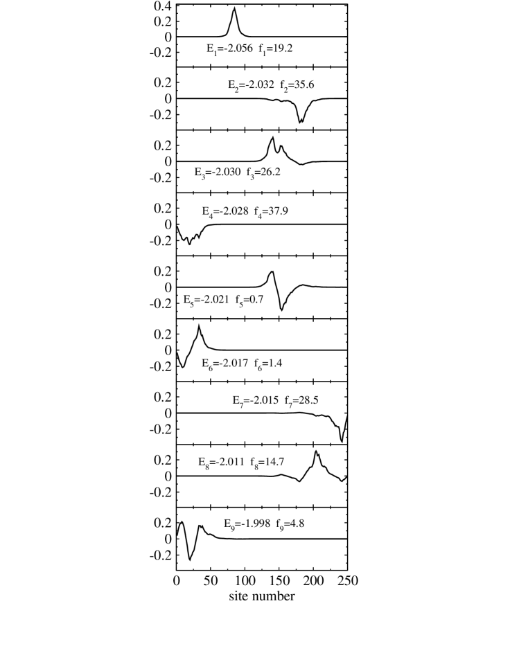
Figure 1: The typical realization of the low-energy eigenfunctions of the Hamiltonian (1) for the 250 sites linear and the disorder degree $\Delta/|J|=0.1$. Each plot also shows the corresponding energy of the state $E_{\nu}$ (in units of $|J|$) and its oscillator strength $f_{\nu}$.

III.1 Heuristic arguments

Before doing the detailed statistical analyses let us look at a typical realization of the eigenstates (for a fixed stochastic distribution of site energies). Figure 1 presents an example showing the nine lowest eigenfunctions $\varphi_{\nu}$ (these are real in our case) and the corresponding eigenenergies $E_{\nu}$. This set of wave functions was obtained for 250 sites chain in the NN model for the disorder degree $\Delta/|J|=0.1$. Each plot also displays the corresponding oscillator strength $f_{\nu}=\left(\sum_{i=1}^{\cal N}\varphi_{\nu i}\right)^{2}.$

Several typical features of the lower eigenstates can clearly be seen from Fig. 1. First, all eigenfunctions are well localized at different segments of the chain. The lengths of these segments $N$ are smaller than the total chain length ${\cal N}$. Some of the eigenfunctions are localized at the same segment (e. g. manifold of states 4, 6 and 9) and weakly overlap with the other states. Second, one of the states of each particular (local) manifold has no nodes within its localization segment and hence have high oscillator strength (e. g. state 4) while the other wave functions from the manifold (e. g. states 6 and 9) have nodes within the segment and low oscillator strengths. This allows to classify such states as local ground and local excited states respectively. These states are similar to the states of a regular non-disordered chain (see Eq. (5) at $k=1$ and $k=2,\,3$). Finally, it is important to note that a local ground state can have higher energy than a local excited state which is localized at a different segment. For example, the local ground state $7$ has higher energy ($E_{7}=-2.015|J|$) than the local excited states $6$ ($E_{6}=-2.021|J|$) and $5$ ($E_{5}=-2.017|J|$). This raises the question about the correlations between the local ground and excited states from one manifold, on the one hand, and between the states from different manifolds, on the other hand.

It is clear from these arguments that grouping the states together into local manifolds is a principal problem; correct criteria are needed to select the states which are localized at the chain segments. When such grouping is done the statistical analysis we are interested in becomes simple.

III.2 Selection criteria

To select the states which are localized at the same segment first we need to find the local ground states. Such states $\varphi_{\nu}$ satisfy the inequality:

$$\left|\sum_{i}\varphi_{\nu i}\,|\varphi_{\nu i}|\right|\geq C_{0}\ .$$ (10)

For the constant $C_{0}$ we use the value $C_{0}=0.95$, seeking, in other words, for the states which contain at least 95% of the wave function density in the main peak. The states $1-4$ and $7$ in the Fig. 1 meet this criterion and can be considered as the local ground states.

Then we find all local excited states. In order to do this we proceed as follows: for each local ground state $\nu$ ($\nu=1-4,7$ in our example) we seek for the states $\nu^{\prime}\neq\nu$ which are localized at the same segment as the state $\nu$. These (local excited) states should simultaneously meet two criteria. The first is similar to the criterion given by Eq. (10):

$$\left|\sum_{i}\varphi_{\nu i}\,|\varphi_{\nu^{\prime}i}|\right|\geq C_{1}\ ,$$ (11)

where $i$ runs over all sites of the chain. The value for the cut-off constant $C_{1}$ will be discussed later. The second criterion is to be applied to the Fourier transforms $\phi_{\nu}$ corresponding to the wave functions $\varphi_{\nu}$:

$$\sum_{q}|\phi_{\nu q}|\,|\phi_{\nu^{\prime}q}|\geq C_{2}\ .$$ (12)

The later is necessary to drop rapidly oscillating states $\nu^{\prime}$, envelope functions of which are localized within the same segment as the considered ground state $\nu$. The energy of such states is in the vicinity of the exciton band maximum. Their spatial extension is of the same order of magnitude as the localization length of the low-energy states, so these high-energy states often meet the criterion (11).

The reasonable values for the cut-off parameters $C_{1}$ and $C_{2}$ can be estimated by considering the states of a rectangular quantum well. In the limiting case of an infinitely deep quantum well the overlap integral for the ground state (given by Eq. (5) at $k=1$) and the module of the first excited state (Eq. (5) at $k=2$) is equal to $I_{m}=8/3\pi\approx 0.85$. In the more general case of a finite rectangular well the value of this integral depends on the well depth and width. It varies from about $I_{m}$ (for a very deep excited state) to zero. Small values of the integral occur for very extended excited states that are just appeared in the well.

Consider the well for which the probability to find the particle in the well equals $0.95$ for the ground state, then for the first excited state this probability equals about $0.75$. The overlap integral of the type (11) for these states is about $0.8$. This value gives an estimate for the parameter $C_{1}$. The overlap integral of the moduli of the Fourier transforms of these states is about $0.56$, which gives an estimate for the $C_{2}$. For our estimations we considered the limiting case of a rectangular well potential which varies infinitely rapidly at the well boundaries. In a smoother potential the values of the overlap integrals can be smaller. To account for this we use more relaxed cut-off criteria with $C_{1}=0.7$ and $C_{2}=0.5$. It is also worth noting that straightforward calculations revealed only weak quantitative dependence of the final results on the values of the cut-off parameters (see Appendix).

Applying the criteria (11) and (12) to our sample set of eigenfunctions we find the following pairs of the local ground and first excited states: $\{3,5\}$ and $\{4,6\}$. This finding looks reasonable (see Fig 1). The states $4$ and $9$ also meet the above criteria. Fig. 1 shows that the state $9$ has two well defined nodes within the segment of localization of the local ground state $4$. It therefore can be referred to as the second local excited state. However, the second and higher local excited states will not be the subject of the present study. Such higher excited states are usually localized at more extended segments and can not be associated with a particular local ground state.

III.3 Statistics of the local ground states

Figure 1 clearly shows that the spatial extension of a local ground state (its localization length $N$) fluctuates from one state to another. Different quantities can be used to characterize the extension of a wave function: (i) the inverse participation ratio (IPR), defined as $\sum_{i}\,|\varphi_{\nu i}|^{4}$,  (ii) the mean-square displacement $\left[\sum_{i}\,|\varphi_{\nu i}|^{2}(i-\bar{i})^{2}\right]^{1/2}$, where $\bar{i}=\sum_{i}\,|\varphi_{\nu i}|^{2}\,i$,  (iii) the inverse of the Lyapunov exponent $\lambda_{\nu}=-\lim_{i\rightarrow\infty}\,(1/2i)\ln|\varphi_{\nu i}|^{2}$ and others. Kramer93 Although these quantities yield slightly different localization lengths, they are of the order of the number of sites over which the wave function is extended.

For the local ground state, an alternative quantity can be used as the measure of its extension. According to Eq. (9), the oscillator strength of the ground state of the ideal linear chain is about the same as the chain length. In other words, $f_{\nu}$ also carries information about the extension of the corresponding local ground state wavefunction $\varphi_{\nu}$. Furthermore, the oscillator strength can be measured experimentally, e.g. it can be determined from the exciton spontaneous decay kinetics Fidder93a ; Fidder91 ). For this reason we use the oscillator strength as the measure of localization of the local ground states.

The number of sites in the chain ${\cal N}$ should be much larger than the typical oscillator strength $f^{*}$ (${\cal N}\gg f^{*}$). As $f^{*}$ was found to be of the order of several tens for the disorder degree $\Delta/|J|=0.1$ and decreases with increasing $\Delta/|J|$, we consider $400$ cites chains (${\cal N}=400$). Applying the selection criterion (10) we calculated the $f$-distribution for the local ground states. The result obtained in the NN approximation is presented in the Fig. 2. Figure 2(a) shows the (typical) oscillator strength distribution $P(f)$ obtained for a 400 sites chain by averaging over 5000 realizations of disorder for the disorder degree $\Delta/|J|=0.1$. The main features of the distribution are clearly seen in the figure: (i) - asymmetry with respect to the expectation value of $f$, (ii) - long tail in the large lengths region, and, on the contrary, (iii) - steep drop off in the region of small values of $f$.

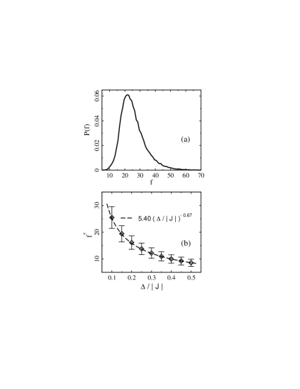
Figure 2: (a) - The distribution $P(f)$ of the local ground state oscillator strength $f$ obtained for a 400 sites chain and the disorder degree $\Delta/|J|=0.1$ (5000 realizations of disorder was considered, each point of the distribution is averaged over the interval (accumulation length) $\delta=1$). (b) - the disorder degree scaling of the first momentum $f^{*}\equiv\int dfP(f)f$ obtained for a 400 sites chain (300 realizations of disorder was considered for each value of the disorder degree $\Delta/|J|$). Diamonds present the numerical data while the dashed line gives the best power-law fit. Error bars show the standard deviation of the distribution, $\sigma\equiv[\int dfP(f)(f-f^{*})^{2}]^{1/2}$.

Figure  2(b) presents the disorder degree scaling of the first momentum of the $P(f)$ distribution, $f^{*}\equiv\int dfP(f)f$. Error bars in Fig. 2(b) show the standard deviation $\sigma\equiv[\int dfP(f)(f-f^{*})^{2}]^{1/2}$. The best fit (dashed line) to the numerical data (diamonds) is given by the power-law approximation in the form

$$f^{*}\approx 5.40\,\left({\Delta\over|J|}\right)^{-0.67}\ .$$ (13)

The theoretical estimate for the localization length was presented in Refs. Malyshev91, ; Malyshev95, (see also Ref. Bakalis00, ) and was based on the following arguments: An exciton localized at a segment of size $N^{*}$ feels a reduced (exchange-narrowed) disorder $\sigma\equiv\Delta/\sqrt{N^{*}}$; Knapp84 this reduced disorder degree must be of the same order of magnitude as the energy separation between the two lowest local exciton levels, $E_{2}^{*}-E_{1}^{*}=3\pi^{2}|J|/N^{*}$. Indeed, if $E_{2}^{*}-E_{1}^{*}$ is smaller than $\sigma$ the two levels would be strongly mixed by disorder and the corresponding exciton wave functions would tend to reduce their extension. On the contrary, if $E_{2}^{*}-E_{1}^{*}$ exceeds $\sigma$ then the disorder is perturbative and the wave functions would tend to increase their extension. Thus, the equality $E_{2}^{*}-E_{1}^{*}=\sigma$ gives the self-consistent relationship between the spatial extension of the exciton wave functions and the disorder degree which the localized exciton feels. This relationship provides an estimate for the localization length $N^{*}$:

$$N^{*}\approx\left({3\pi^{2}|J|\over\Delta}\right)^{2/3}\approx 9.57\,\left({\Delta\over|J|}\right)^{-2/3}\ .$$ (14)

This theoretical scaling law is in good agreement with the scaling law of $f^{*}$ obtained numerically, the latter being smaller by the factor of about $2$. This is not surprising because, according to Eq. (9), the oscillator strength is smaller than the localization length. The mean localization length $N^{*}$ was also calculated ($N$ was defined as the number of sites under the main peak of the wavefunction, for which $|\varphi_{\nu i}|/max_{i}\{|\varphi_{\nu i}|\}>0.1$). The mean oscillator strength $f^{*}$ was found to be proportional to $N^{*}$: $f^{*}=cN^{*}$, where $c\approx 0.66$ . Rewriting Eq. (13) in terms of $N^{*}$ yields $N^{*}\approx 8.71\,(\Delta/|J|)^{-0.67}$, which is in excellent agreement with the theoretical estimate (14).

III.4 Statistics of the energy levels near the lower exciton band edge

In this section we analyze two eigenenergy distributions which are of primary interest for us. The first is the distribution of the energy spacing between the local ground states of different segments, while the second is the distribution of the energy spacing between the local excited and ground states of the same segment. We denote them as $P_{11}(\delta E)$ and $P_{21}(\delta E)$ respectively. Utilizing the selection criteria of Sec. III.2 (Eqs. (10)-(12)) we calculated these distributions. The results of these calculations are presented in Figs. 3 and 4.

Figures 3(a) and 3(b) present the (typical) distribution of the energy spacing between the local ground states $P_{11}(\delta E)$ obtained for a 400 sites chain by averaging over 5000 realization of disorder. The disorder degree $\Delta/|J|=0.1$ and the NN model was used. The plot (a) shows $P_{11}(\delta E)$ for the adjacent (most overlapping) ground states only. These states were selected by the criterion $\sum_{i}\,|\varphi_{\nu i}|\,|\varphi_{\nu^{\prime}i}|\geq 0.01$. The distribution presented in Fig. 3(b), was obtained without the above restriction, i. e. for all ground states.

The two distributions are very close to each other. The most important feature of both is that they are nearly symmetric with respect to zero energy spacing, in other words, they are characterized by zero mean. The disorder degree scaling of the corresponding first momenta (not presented here) confirms this fact. A weakly pronounced downfall in the vicinity of the zero energy spacing of the distribution for the adjacent states (plot (a)) is due to the repulsion of close energy levels of the overlapping states. Similarly, two degenerate states in a camel’s back potential are split into a doublet when interaction between them is considered. This downfall tends to disappear when all ground state are considered (see Fig. 3(b)).

The plot (c) of Fig. 3 shows the disorder degree scaling of the standard deviation of the distribution $P_{11}(\delta E)$, $\sigma_{11}=[\int d(\delta E)(\delta E)^{2}P_{11}(\delta E)]^{1/2}$, calculated for all ground states. The best power-law fit (dashed line) to the numerical data (diamonds) is given by

$$\sigma_{11}\approx 0.67\;|J|\,\left(\Delta\over|J|\right)^{1.33}\ .$$ (15)

The scaling law of $\sigma_{11}$ is close to the scaling law of the one-exciton absorption linewidth Schreiber82 ; Koehler89 ; Boukahil90 , which supports the idea that these quantities are proportional to each other.

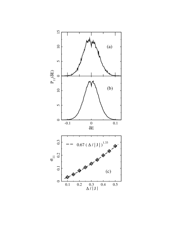
Figure 3: (a,b) - The distributions of the energy spacing between the local ground states obtained for a 400 sites chain and the disorder degree $\Delta/|J|=0.1$ (5000 realizations of disorder was considered, each point of the distributions is averaged over the interval (accumulation length) $\delta=0.0015$). The plot (a) shows the distribution $P_{11}(\delta E)$ for the adjacent local ground states (with the overlap integral $\sum_{i}\,|\varphi_{\nu i}|\,|\varphi_{\nu^{\prime}i}|\geq 0.01$). The distribution shown in the plot (b) was calculated for all local ground states. (c) - the disorder degree scaling of the standard deviation $\sigma_{11}=[\int d(\delta E)(\delta E)^{2}P_{11}(\delta E)]^{1/2}$ obtained for a 400 sites chain (300 realizations of disorder was considered for each point). Diamonds present the numerical data while the dashed line gives the best power-law fit. All energies are in units of $|J|$.

Figure 4(a) shows the (typical) distribution $P_{21}(\delta E)$ of the energy spacing between the ground and first excited states localized within the same segment. This distribution was obtained for the same set of parameters (${\cal N}=400$, $\Delta/|J|=0.1$, 10000 realizations). In contrast to the $P_{11}(\delta E)$ (Fig. 3(a, b)) the distribution $P_{21}(\delta E)$ is asymmetric with respect to the expectation value of $\delta E$. The high-energy-spacing shoulder of this distribution is much longer than the shoulder in the region of small values of $\delta E$. However, the most important features of the $P_{21}(\delta E)$ are the following. First, it is characterized by non-zero mean, which unambiguously shows that the energies of the pairs of states that are localized within the same segment are highly correlated, in the sense that they undergo repulsion resulting in the local discrete energy structure. Second, the distribution $P_{21}(\delta E)$ drops down rapidly at $\delta E\simeq{\delta E}_{c}$ and vanishes below the energy ${\delta E}_{c}$. For the particular value of the disorder degree $\Delta/|J|=0.1$ this energy is small compared to the characteristic energy scale in the figure ($\delta E_{c}\approx 0.001$). The log-linear insert presents a blow-up of the distribution function $P_{21}(\delta E)$ in the region of very small energy spacings $\delta E\sim\delta E_{c}$ (each point is averaged over the interval $\delta=0.0005$ in the insert).

The quantity of interest in the present case is the first momentum of the distribution $P_{21}(\delta E)$. Denote it as $E^{*}_{2}-E^{*}_{1}$. The physical meaning of this quantity is clear: it is the mean energy spacing between the levels of a local manifold. The calculated disorder scaling of $E^{*}_{2}-E^{*}_{1}=\int d(\delta E)P_{21}(\delta E)\delta E$ (diamonds) is shown in Fig. 4(b) together with the best power-law fit (dashed line) to the numerical data:

$$E^{*}_{2}-E^{*}_{1}\approx 0.40\;|J|\,\left(\Delta\over|J|\right)^{1.36}\ .$$ (16)

Note that the disorder scaling laws for $E^{*}_{2}-E^{*}_{1}$ and $\sigma_{11}$ are very close to each other. The theoretical estimate of the $E^{*}_{2}-E^{*}_{1}$ scaling was obtained in Refs. Malyshev91, ; Malyshev95, :

$$E^{*}_{2}-E^{*}_{1}\approx(3\pi^{2})^{-1/3}\;|J|\,\left({\Delta\over|J|}\right)^{4/3}\approx 0.32\;|J|\,\left({\Delta\over|J|}\right)^{4/3}\ ,$$ (17)

and agrees excellently with the calculated behavior. This result was also obtained numerically in Ref. Bakalis99, , where the detuning between bleaching and induced absorption of the pump-probe spectrum was simulated. This detuning is a good measure for the exciton delocalization length Malyshev95 ; Bakalis99 .

It is remarkable that rescaling of the numerical data for $E^{*}_{2}-E^{*}_{1}$ in terms of $f^{*}$ gives $E^{*}_{2}-E^{*}_{1}\sim(1/f^{*})^{2}$, the proportionality that holds for an ideal linear chain of length $f^{*}$. This is yet another confirmation of the existence of the local discrete energy structure of a weakly localized Frenkel exciton near the lower band edge.

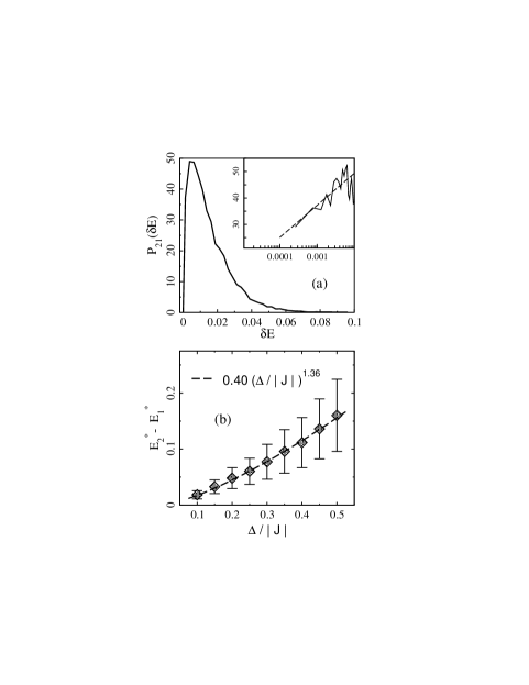
Figure 4: (a) - The distribution of the energy spacing between the local ground and first excited states of the same segment, $P_{21}(\delta E)$, obtained for a 400 sites chain and the disorder degree $\Delta/|J|=0.1$ (10000 realizations of disorder is considered, each point of the distributions is averaged over the interval (accumulation length) $\delta=0.0025$). The insert shows the behavior of the distribution function $P_{21}(\delta E)$ in the region of very small energy spacings $\delta E$ (each point is averaged over the interval $\delta=0.0005$) (b) - The disorder degree scaling of the first momentum $E^{*}_{2}-E^{*}_{1}\equiv\int d(\delta E)P_{21}(\delta E)\delta E$ obtained for a 400 sites chain (each point is averaged over 300 realizations of disorder). Diamonds present the numerical data while the dashed line gives the best power-law fit. Error bars show the standard deviation of the distribution, $\sigma_{21}=[\int d(\delta E)P_{21}(\delta E)(E_{2}^{*}-E_{1}^{*}-\delta E)^{2}]^{1/2}$. All energies are in units of $|J|$.

It is also of interest to compare the mean $E_{2}^{*}-E_{1}^{*}$ of the $P_{21}(\delta E)$ distribution with the standard deviation $\sigma_{11}$ of the $P_{11}(\delta E)$ distribution. The figures 3(c) and 4(b) as well as the equations (15) and (17) for these quantities show that $E_{2}^{*}-E_{1}^{*}<\sigma_{11}$. This finding clarifies the fact that the local discrete energy structure can not be seen neither in the density of states (see Refs. Fidder93a, ; Fidder91, ; Schreiber82, ; Kozlov98, ) nor in the linear absorption spectra (see Refs. Fidder93a, ; Malyshev99, ; Knapp84, ; Fidder91, ); the energy fluctuations of the local ground states exceed the characteristic energy scale of the local energy structure, hence, the fine local structure is hidden by the inhomogeneous broadening of the local ground states.

The effect of level repulsion is well known from the studies of spectra of complex systems, such as nuclei. Mehta90 These studies are often based on the random matrix theory (RMT). Mehta90 In particular, this theory predicts level repulsion for the eigenvalues of a real symmetric matrix chosen at random from the Gaussian orthogonal ensemble, i.e. when all matrix elements are Gaussian stochastic variables statistically independent of each other. Despite a seeming similarity of this result and ours they cannot be directly related to each other. First, the off-diagonal matrix element of the Hamiltonian (1) are not stochastic variables while they are in the random matrix theory. Moreover, in the RMT the off-diagonal elements have zero mean, while in the Hamiltonian (1) they are all negative. Second, we found the well-pronounced effect of level repulsion only for a sub-ensemble of levels. Simulations for the entire set of levels show almost no level repulsion in the vicinity of the band bottom (see Fig. 5).

III.5 Long-range coupling effects

Complete set of the above mentioned simulations was also performed for the exact DD coupling model. It was found that $f^{*}$, $\sigma_{11}$, and $E^{*}_{2}-E^{*}_{1}$ are strongly affected by the long-range dipole-dipole terms. The following expressions give the best fit to the numerical data:

$$f^{*}\approx 9.74\,\left({|J|\over\Delta}\right)^{0.80}\ ,$$ (18)

$$\sigma_{11}\approx 0.50\;|J|\,\left({|J|\over\Delta}\right)^{1.36}\ ,$$ (19)

$$E^{*}_{2}-E^{*}_{1}\approx 0.37\;|J|\,\left({\Delta\over|J|}\right)^{1.53}.$$ (20)

Unlike the NN model case, the rescaling formula $E^{*}_{2}-E^{*}_{1}\sim(1/f^{*})^{2}$ does not hold for the exact DD model. This finding is not surprising, as it agrees with the change in the exciton energy spectrum of a regular chain in the DD approximation as compared to that obtained in the NN approximation (see Eqs. (6) and (7)). The logarithmic factor in Eq. (6) is breaking the $E^{*}_{2}-E^{*}_{1}\sim(1/f^{*})^{2}$ dependence. The deviation of the exponents $0.80$ and $1.53$ in Eqs. (18) and (20) from the NN model values $2/3$ and $4/3$ is also due to this factor. Malyshev95 As a matter of fact, the power-law approximation is not adequate for the exact model. Using the exact low-energy spectrum of the 1D localized exciton and the rule described at the end of Sec. III.3), the authors of Ref. Malyshev95, obtained the correct equation for the localization length $N^{*}$:

$$\frac{N^{*\,3/2}}{\ln N^{*}+a}=b\,\frac{|J|}{\Delta}$$ (21)

with $a=3/2-ln(2^{4/3}\pi)\approx-0.57$ and $b=3\pi^{2}\approx 30$.

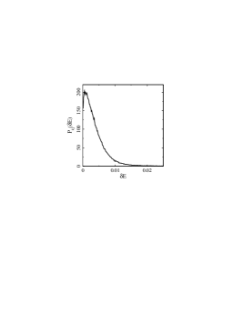
Figure 5: The distribution of the energy spacing between levels in the vicinity of the exciton band bottom, $P_{ij}(\delta E)$, obtained for a 400 sites chain and the disorder degree $\Delta/|J|=0.1$ (5000 realizations of disorder was considered, each point of the distributions is averaged over the interval (accumulation length) $\delta=0.00015$). All energies are in units of $|J|$. Note that that this distribution shows almost no level repulsion.

Straightforward comparison of the scaling laws of the quantities $f^{*}$ and $N^{*}$ (the latter is defined as the number of sites under the main peak of the wavefunction, see also the end of Sec. III.3), shows that, like in the NN model, these quantities are proportional to each other $f^{*}=c\,N^{*}$, where $c\approx 0.62$. Fitting Eq. (21) to the numerical data for $c^{-1}f^{*}$, the following optimal values of the parameters were found: $a=-0.54$ and $b=25.1$. These values are in excellent agreement with the theory.

In conclusion to this section we would like to comment on the disorder scaling law of the exciton-radiative-rate enhancement factor which was obtained numerically in Ref. Fidder91, for the exact dipole-dipole coupling model. This factor is introduced as follows: define the average oscillator strength per state at energy $E$: $\mu^{2}(E)=A(E)/\rho(E)$, where $A(E)$ and $\rho(E)$ are the absorption spectrum and the density of exciton states respectively, then $max[\mu^{2}(E)]$ is an effective measure for the enhancement of the radiative rate. This quantity also contains information about the spatial extension of the exciton states coupled to the light. Fidder91 The authors of Ref. Fidder91, found from their simulations that $max[\mu^{2}(E)]\sim(|J|/\Delta)^{0.74}$. The exponent of this scaling law, $0.74$, differs from the value obtained in our simulations, $0.80$ (Eq. (18)). We believe that this discrepancy of the order of 10% originates in the different definitions of $f^{*}$ used in our study and in Ref. Fidder91, .

IV Summary and concluding remarks

In this paper we discuss the statistics of energy levels of the 1D Frenkel Hamiltonian with on-site randomness near the lower band edge. The heuristic arguments on the existence of the local discrete energy structure, which were put forward in Refs. Malyshev91, and Malyshev95, are confirmed by the detailed statistical study. Selecting the states by means of the overlap integrals we find that the energy levels of the well overlapping states indeed undergo repulsion resulting in the local energy structure which is similar to the structure of an ideal linear chain of the reduced length $N^{*}$ (localization length). The lowest state of each set has no nodes within the localization segment and therefore can be interpreted as the local ground state, while the next state in a set has a node within the segment and is the first local excited state, etc. The average energy spacing of the local ground and first excited states obtained within the framework of the NN model follows the $(1/N^{*})^{2}$ dependence that holds for an ideal chain of length $N^{*}$.

On the contrary, the energy spacing of the non-overlapping local ground states is characterized by zero mean and distributed in the energy interval that is of the same order of magnitude as the mean energy spacing of the local energy structure. Therefore, the local energy structure appears to be hidden in the density of states Fidder93a ; Fidder91 ; Schreiber82 and in linear absorption spectra as well. Fidder93a ; Knapp84 ; Fidder91 ; Schreiber82 Nevertheless, this structure can be revealed by the pump-probe spectroscopy sharing two-exciton states. Malyshev95 ; Bakalis99 Indeed, due to fermionic nature of 1D Frenkel excitons, Chesnut63 ; Avetisyan85 ; Juzeliunas88 ; Spano91 one-to-two and zero-to-one exciton optical transitions involving the states of the same local structure would be blue-shifted with respect to each other. This shift is equal to the energy spacing between the local ground and first excited states. The blue shift of one-to-two and zero-to-one exciton optical transitions in J-aggregates of pseudoisocyanine bromide was observed experimentally Minoshima94 ; Fidder93b providing unambiguous confirmation of the existence of the local discrete energy structure in the vicinity of the exciton band minimum.

Appendix A Effect of the cut-off parameters

In this section the weak dependence of the results on the cut-off parameters $C_{1}$ and $C_{2}$ is illustrated. Figure 6 shows several distributions $P_{21}(\delta E)$ calculated for different sets of the cut-off parameters: $C_{1}=0.7$, $C_{2}=0.3$ — dash-dotted line, $C_{1}=0.7$, $C_{2}=0.5$ — solid line, $C_{1}=0.8$, $C_{2}=0.3$ — dotted line, $C_{1}=0.8$, $C_{2}=0.5$ — dashed line. These distributions are very close to each other, which results in only weak (less than 15%) quantitative dependence of distribution momenta on the values of the cut-off parameters.

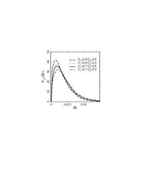
Figure 6: The distribution of the energy spacing between the local ground and first excited states of the same segment, $P_{21}(\delta E)$, obtained for a 200 sites chain and the disorder degree $\Delta/|J|=0.1$ (40000 realizations of disorder was considered, each point of the distributions is averaged over the interval $\delta=0.0025$). The curves are calculated for different sets of the cut-off parameters: $C_{1}=0.7$, $C_{2}=0.3$ — dash-dotted line, $C_{1}=0.7$, $C_{2}=0.5$ — solid line, $C_{1}=0.8$, $C_{2}=0.3$ — dotted line, $C_{1}=0.8$, $C_{2}=0.5$ — dashed line. All energies are in units of $|J|$.

References

- (1) N. F. Mott and W. D. Twose, Adv. Phys. 10, 107 (1961).
- (2) E. Abrahams, P. W. Anderson, D. C. Licciardello, and V. Ramakrishnan, Phys. Rev. Lett. 42, 673 (1979).
- (3) B. Kramer and A. MacKinnon, Rep. Prog. Phys. 56, 1469 (1993).
- (4) J. C. Flores, J. Phys.: Condens. Matter 1, 8471 (1989).
- (5) D. H. Dunlap, H.-L. Wu, and P. Phillips, Phys. Rev. Lett. 65, 88 (1990).
- (6) V. Bellani, E. Diez, R. Hey, L. Toni, L. Tarricone, G. B. Parravicini, F. Domínguez-Adame, and R. Gómez-Alcalá, Phys. Rev. Lett. 82, 2159 (1999).
- (7) H. Fidder, Thesis, Groningen, 1993.
- (8) F. C. Spano and J. Knoester, in Advances in Magnetic and Optical Resonance, Vol. 18, ed. W. S. Warren (Academic, New York, 1994), p. 117.
- (9) J. Knoester and F. C. Spano, in J-aggregates, ed. T. Kobayashi (World Scientific, Singapur, 1996), p. 111.
- (10) V. A. Malyshev, Opt. Spektr. 71, 873 (1991) [Opt. Spectr. 71, 505 (1991)]; J. Lumin. 55, 225 (1993).
- (11) V. Malyshev and P. Moreno, Phys. Rev. B 51, 14, 587 (1995).
- (12) M. Shimizu, S. Suto, T. Goto, A. Watanabe, and M. Matsuda, Phys. Rev. B 58, 5032 (1998).
- (13) V. A. Malyshev, A. Rodríguez, and F. Domínguez-Adame, Phys. Rev. B 60, 14140 (1999).
- (14) L. Bakalis and J. Knoester, J. Phys. Chem. B 103, 6620 (1999); J. Lumin. 83-84, 115 (1999).
- (15) E. W. Knapp, Chem. Phys. 85, 73 (1984).
- (16) K. Minoshima, M. Taiji, K. Misawa, T. Kobayashi, Chem. Phys. Lett. 218 (1994) 67.
- (17) L. Bakalis and J. Knoester, J. Lumin. 87-89, 66 (2000).
- (18) A. S. Davydov, Theory of Molecular Excitons (Plenum, New York, 1971).
- (19) H. Fidder, J. Knoester, and D. A. Wiersma, J. Chem. Phys. 95, 7880 (1991).
- (20) M. Schreiber and Y. Toyozawa, J. Phys. Soc. Jpn. 51, 1528 (1982).
- (21) J. Köhler, A. M. Jayannavar and P. Reineker, Z. Phys. B 75, 451 (1989).
- (22) A. Boukahil and D. L. Huber, J. Lumin. 45, 13 (1990).
- (23) G. G. Kozlov, V. A. Malyshev, F. Domínguez-Adame, and A. Rodríguez, Phys. Rev. B 58, 5367 (1998).
- (24) M. L. Mehta, Random Matrices (Academic Press, Boston - San Diego - New York - London - Sydney - Tokio - Toronto, 1990).
- (25) D. B. Chesnut and A. Suna, J. Chem. Phys. 39, 146 (1963).
- (26) Yu. A. Avetisyan, A. I. Zaitsev and V. A. Malyshev, Opt. Spektr. 59, 967 (1985) [Opt. Spectr. 59, 582 (1985)].
- (27) G. Juzeliunas, Z. Phys. D 8, 379 (1988).
- (28) F. C. Spano, Phys. Rev. Lett. 67, 3424 (1991); Phys. Rev. Lett. (E) 68, 2976 (1992).
- (29) H. Fidder, J. Knoester, and D. A. Wiersma, J. Chem. Phys. 98, 6564 (1993).