Abstract

We discuss a new entangled state that has been observed in the conduction across a quantum dot. At Coulomb blockade, electrons from the contacts correlate strongly to those localized in the dot, due to cotunneling processes. Because of the strong Coulomb repulsion on the dot, its electron number is unchanged w.r.to the dot in isolation, but the total spin is fully or partly compensated. In a dot with $N=\>\>even$ at the singlet-triplet crossing, which occurs in large magnetic field, Kondo correlations lead to a total spin $S=1/2$.

Compensation of the spin of a quantum dot at Coulomb blockade

Kondo correlation with the contacts leads to a macroscopic separation of the charge from the spin in the dot

Introduction

A very special kind of Macroscopic Quantum Coherence has been recently measured. This is the Kondo anomaly of the conductance across a quantum dot (QD) polarized at Coulomb blockade (CB) [1, 2, 3]. Due to confinement, Coulomb correlations between electrons added to a QD are strong. An appropriate choice of the gate voltage $V_{g}$ blocks direct sequential tunneling, what is called Coulomb blockade regime[4]. If coupling between the QD and the leads is not weak and the temperature is low enough, an anomaly appears in the differential conductance at zero voltage bias. Kondo correlations are established by cotunneling processes. This leads to a macroscopic ground state (GS) with very peculiar properties, in which the dot and the contacts are entangled.

Kondo conduction is a well known phenomenon occurring in non magnetic metals with diluted magnetic impurities[5]. Typical examples are $Fe$ in $Cu$ or $Mn$ in $Ag$: a minimum in the resistivity of the metal occurs in lowering the temperature below $T_{K}$, before saturating to a residual value corresponding to potential (non magnetic ) scattering. Kondo showed that [6] there is a crossover to a correlated state of the system in the neighborhood of $T_{K}$, in which exchange interaction between the conduction electrons and the local moment of the impurity leads to scattering events on the microscopic scale, in which the electronic spin is flipped. This gives rise to a term in the impurity contribution to the resistivity that increases with decreasing temperature. Spin flip can only occur if the spin on the local magnetic moment of the impurity atom changes accordingly, to achieve compensation. This shows up in the disappearance of a Curie-Weiss spin susceptibility which becomes constant at low temperature.

To some extent the conductance across a QD in the CB regime can be regarded as the mesoscopic realization of the same physics[7]. This is not so surprising, as QD have always been referred to as artificial atoms and the contacts provide the delocalized conduction electrons of the host metal.

Of course the energy scales are quite different. Energy level separation in a QD is of the order of $meV$ while it is of two or three orders of magnitude larger for the $d,f$ electronic levels in the impurity atom. This implies that the temperature scale (the Kondo temperature $T_{K}$ ) is correspondingly reduced from tens of $K$ to $100mK$ and below. Also, because the anomalous contribution to the conductance stems from cotunneling processes, the internal structure of the QD is of big relevance. Coulomb interaction is dominant in QD, so that the levels involved are many particle levels which strongly depend on the number of electrons added to the dot $N$ by means of a gate voltage $V_{g}$.

In this sense one should be cautious when extending the single impurity Anderson model to the dot case[8]. The model describes localized single electron levels with an onsite Coulomb repulsion $U$, in hybridization with delocalized conduction electrons. It is important that the order of magnitude of $U$ is the same for both the magnetic atom and the QD, so that, in the dot case, we are always in the large $U$ limit, what makes the experimental observation even more striking. In particular, the Kondo peak is observed in a QD in the CB region where conductance is otherwise exponentially small. This is because QDs can be tuned within a very wide range of parameter values and the experiment on Kondo conduction is equivalent to the measurement of one single impurity in the metal host.

As we will show, the investigation of the analogies between the two systems is very fruitful, because new features arise in QD, that are not found when localized moments in diluted alloys are studied.

One example is Kondo conduction in a magnetic field[9]. Because orbital effects are very important in a QD when a magnetic field is applied, the energy scale for the Zeeman spin splitting is not the same as the energy scale for level separation in a QD in magnetic field. This implies that, in diluted alloys, a magnetic field $B$ is always disruptive for Kondo correlations because it lifts the degeneracy of the levels, which is required for the spin flip scattering events. On the dot side, it may even produce crossings of the levels of the dot, which could favour Kondo conductance. We will discuss an example of this in Sect. 2.

The spectroscopy of a QD is usually performed in terms of transport measurements[10]. Two electrodes are attached to the QD and the low-temperature zero-bias conductance is monitored. When the gate voltage $V_{g}$ changes, the conductance undergoes a series of peaks at zero source-drain voltage $V_{sd}$ each time the increase in $V_{g}$ matches the chemical potential for adding an extra electron to the dot (Coulomb oscillations). In between two peaks, the number of particles on the QD is fixed (CB regime)( see Fig. 1 for the setup $(a)$ and for a schematic grey-scale drawing of the conductance $vs$ $V_{g}$ and $V_{sd}$ $(b)$) . Contributions to the current at CB are fourth order in the transmission amplitude and can be very small (white regions in Fig.1 b)). In these conditions the total spin of the dot $S$ is the only left dynamical variable, as in a magnetic impurity.

Provided this spin is not a singlet, it can become strongly coupled to the spin density of the contacts electrons if $T<T_{K}$ and the leads are not weakly linked. The correlated state gives rise to non perturbative differential conduction at zero voltage bias, fairly independent of the value of $V_{g}$ within the CB plateaux.

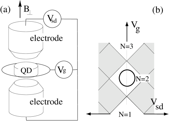
Figure 1: $a)$ Geometry of a vertical QD. $b)$ grey scale picture of the conductance versus gate voltage $V_{g}$ and source-drain voltage $V_{sd}$. In white areas the conductance is vanishingly small.

The first observations were in dots at CB with an odd number of electrons [1, 2]. The GS is a doublet and coupling to the contacts in the CB region generates the Abrikosov-Suhl resonance at the Fermi energy $\mu\equiv\epsilon_{F}$ of the contacts which gives a peak in the differential conductance at zero bias due to cotunneling across the QD.

In Sect. 1 we review the features of the single impurity Anderson model which are at the basis of the physics involved in the Kondo correlated state for QDs with an odd number of electrons. The level of the localized impurity is doubly degenerate and located deeply below $\mu$ but double occupancy of this level would cost an energy much larger than $\mu$. We show that, in the limit of strong onsite repulsion $U$, in spite of the coupling to the leads, occupation of the impurity level is frozen. In addition to the disappearance of the charge degree of freedom, a singlet state is generated on the impurity, with the help of the conduction electrons. In the symmetrical case, the fixed point GS has $(N=1,S=0$). Spin-charge separation occurs.

Dots at CB with an even number of electrons are not expected to give Kondo conduction because the GS is supposed to be a singlet already. A notable exception is when the GS has higher total spin. In dots with $N=4$ and $N=6$ Hund’s rule states that the GS is a triplet. This is turned into a singlet by applying a small $B$ ( denoted “TS crossing” hereafter).

In Sect. 2 we consider the case of a realistic isolated QD with few electrons using exact diagonalization methods [11]. A magnetic field $B_{\perp}$, orthogonal to the dot is applied. This produces large orbital changes in the electronic states and, eventually, crossing of levels. The Kondo effect expected for $S=1$ is strongly enhanced due to this crossing and the anomalous conductance at zero voltage has been recently observed [9]. The very peculiar physics at the TS crossing is under consideration at present[12, 13].

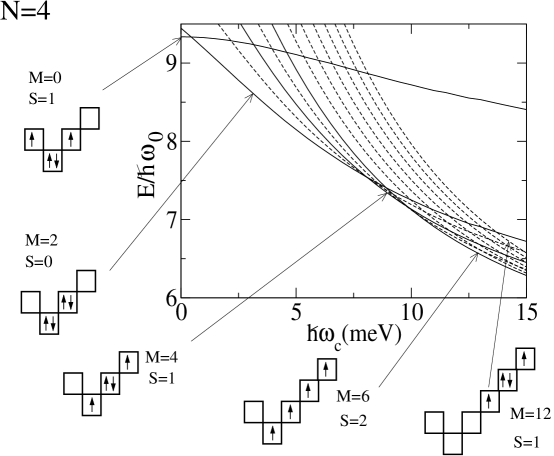
Figure 2: Energy levels of an isolated QD with $N=4$ electrons $vs.$ a magnetic field orthogonal to the dot. The total orbital angular momentum and the total spin of the different GSs are shown, together with the configuration of the Slater determinant which has the highest projection onto the GS.

But there is another possibility of Kondo conductance which has been studied in ref[14]. Increasing $B$ quite substantially, the dot undergoes a new transition from the singlet to triplet state because of orbital effects ( denoted ST crossing hereafter), in which the Zeeman spin splitting cannot be ignored. This changes the properties of the GS in a peculiar way, leading to an even charge on the dot with total spin $\frac{1}{2}$.

1 From the symmetric Anderson model to the impurity spin dynamics

We refer to a QD connected to the leads in the CB regime, in the limit of the Coulomb interaction being very large. As discussed in the introduction, the dot charge degree of freedom is frozen out, what leaves the dot total spin $S$ as the only dynamical variable. The charge-spin separation emerges. This phenomenon is at the basis of the analogy between this system and that of an impurity local moment in a metal alloy. Here we review the main features of the single impurity spin $\frac{1}{2}$ symmetric Anderson model[8]. The path integral formalism by Anderson,Yuval and Hamann [15, 16] is particularly suited to focus on the spin-charge separation in this model.

The Hilbert space of the spin $\frac{1}{2}$ impurity is conveniently described by two fermionic operators, $d_{i}^{\dagger}$, acting on the vacuum $|0\rangle$. The label $i=1,2$ is here a spin label, although it could be a generic label for the two degenerate single particle levels located at energy $\epsilon_{d}$.

The impurity Hamiltonian is:

$$H_{d}=\epsilon_{d}\sum_{i}n_{i}+Un_{1}n_{2}$$ (1)

where $n_{i}=d^{\dagger}_{i}d_{i}$ and $U$ is the strength of the onsite repulsion.

We linearize the conduction electron band $\epsilon_{k}$ close to $\epsilon_{F}$. This allows to write down their Hamiltonian as that of a one-dimensional Fermi gas. To keep contact with the dot picture, we divide the space into a left $(L)$ and a right $(R)$ region:

$$H_{L,R}=\sum_{k\sigma}\epsilon_{k}b_{(L,R)k\sigma}^{\dagger}b_{(L,R)k\sigma}$$ (2)

If $\epsilon_{d}=-U/2$ $w.r.to$ the chemical potential of the conduction electrons $\mu$ (taken as the zero of the single particle energies), the Anderson model which arises is symmetric. In fact, the energies of the empty impurity state,${}^{0}E$, and that of the doubly occupied impurity state, ${}^{2}E=2\epsilon_{d}+U$, are both zero, while the singly occupied impurity level has energy ${}^{1}E=-U/2$.

Finally, the hybridization Hamiltonian between the conduction electrons and the impurity is:

$$H_{t}=\frac{1}{\sqrt{2}}\sum_{k}\{\Gamma^{*}[(b_{Lk\uparrow}^{\dagger}+b_{Rk\uparrow}^{\dagger})d_{1}+(b_{Lk\downarrow}^{\dagger}+b_{Rk\downarrow}^{\dagger})d_{2}]+{\rm h.c.}\}$$ (3)

where all the tunneling amplitudes have been taken equal for simplicity.

We now formulate the quantum dynamics of the system described by eqs.( 1,2,3) using the imaginary time Feynman Path Integral formalism. Following [16], we integrate out the conduction electron fields and we obtain the partition function in terms of the Grassman fields $d,d^{\dagger}$ only ($\hbar=1$ in the following):

$${\cal{Z}}(\mu)\propto\int\Pi_{i}\left(Dd_{i}Dd^{\dagger}_{i}\right)e^{-{\cal{A}}_{d}}\>e^{-\beta|\Gamma|^{2}\sum_{\omega_{m},i}d^{\dagger}_{i}K(i\omega_{m})d_{i}}$$ (4)

where $i\omega_{m}$ are Fermionic Matsubara frequencies,

$${\cal{A}}_{d}=\int_{0}^{\beta}d\tau\left\{\sum_{i}\left[d_{i}^{\dagger}\frac{\partial}{\partial\tau}d_{i}+\epsilon_{d}\>d^{\dagger}_{i}d_{i}\right]+Ud^{\dagger}_{1}d_{1}d^{\dagger}_{2}d_{2}\right\}$$ (5)

and $K(i\omega_{m})$ is:

$$K(i\omega_{m})=\frac{L}{2\pi}\int_{-D}^{D}\frac{dk}{i\omega_{m}+vk}=\frac{L}{2\pi v_{F}}\ln\left(-\frac{v_{F}D+i\omega_{m}}{v_{F}D-i\omega_{m}}\right)\>.$$ (6)

Here $v_{F}$ is the Fermi velocity and $D$ is the band cutoff, symmetrical $w.r.to\>\epsilon_{F}$.

The average impurity occupation number is calculated from the retarded part of the Green function $G^{R}(\omega)$:

$$<n_{i}>=\int_{-\infty}^{\infty}\frac{d\omega}{2\pi}iG^{R}(\omega)\>.$$

$G^{R}(\omega)$ is obtained from $G(i\omega_{m})$ in the limit to real frequencies: $i\omega_{m}\to\omega+i0^{+}$. In the case $U=0$ we have:

$$G_{(0)}^{-1}(i\omega_{m})=i\omega_{m}-\epsilon_{d}+|\Gamma|^{2}K(i\omega_{m})\to\omega-\epsilon_{d}-\frac{\Delta}{\pi}\ln\left|\frac{v_{F}D+\omega}{v_{F}D-\omega}\right|+i\Delta$$

where $\Delta=\pi N(0)|\Gamma|^{2}$ and $N(0)$ is the density of states at the Fermi energy per spin $L/2\pi\hbar v_{F}$.

Assuming that $\tilde{\epsilon}_{d}$ solves the equation $\Re e\{(G^{0})^{-1}\}=0$, we get:

$$<n_{i}>=\int_{-\infty}^{\infty}\frac{d\omega}{2\pi}iG_{0}^{R}(\omega)\approx i\int_{-\infty}^{\infty}\frac{d\omega}{2\pi}\>\frac{1}{\omega-\tilde{\epsilon}_{d}+i\Delta}$$

The imaginary part is odd and vanishes upon integration. The real part gives:

$$<n_{i}>=\int_{-\infty}^{\infty}\frac{d\omega}{\pi}\frac{\Delta}{(\omega-\tilde{\epsilon}_{d})^{2}+\Delta^{2}}=\frac{1}{2}-\frac{1}{\pi}\arctan\frac{\tilde{\epsilon}_{d}}{\Delta}$$ (7)

Eq.(7) describes the Friedel screening around the impurity due to a resonance at $\tilde{\epsilon_{d}}\approx\epsilon_{d}$ of width $\Delta$.

We now discuss the role of the onsite Coulomb interaction. In the large-$U$ limit we have:

$$\exp\int_{0}^{\beta}d\tau\left\{-\epsilon_{d}(n_{1}+n_{2})-Un_{1}n_{2}\right\}$$

$$=e^{\frac{\beta}{U}\epsilon_{d}^{2}}\;\delta(n_{1}+n_{2}+2\epsilon_{d}/U)\>\cdot e^{\frac{U}{4}\int_{0}^{\beta}\;d\tau(n_{1}-n_{2})^{2}}\>\>,$$ (8)

where the delta function implements the constraint of single site occupancy in the symmetric case, $\epsilon_{d}=-U/2$.

The quartic interaction is decoupled by means of a Hubbard-Stratonovitch boson field $X(\tau)$, according to the identity:

$$e^{\frac{U}{4}\int_{0}^{\beta}d\tau(n_{1}-n_{2})^{2}}=\int DXe^{-\frac{1}{4U}\int_{0}^{\beta}d\tau(X^{2}(\tau)+2U(n_{1}-n_{2})X(\tau))}.$$

Having introduced $X(\tau)$, ${\cal Z}(\mu)$ takes the form:

$${\cal{Z}}(\mu)\propto\int DXe^{-\frac{1}{4U}\int_{0}^{\beta}d\tau X^{2}(\tau)}$$

$$\times\int\Pi_{i}\left(Dd_{i}Dd_{i}^{\dagger}e^{-\int_{0}^{\beta}d\tau d\tau^{\prime}d_{i}^{\dagger}(\tau)G^{-1}_{(U)}(\tau-\tau^{\prime})d_{i}(\tau^{\prime})}\right)$$

$$\times\delta(n_{1}+n_{2}-1)\cdot\frac{1}{2}\sum_{j=1,2}e^{(-1)^{j}\int_{0}^{\beta}d\tau[n_{j}-\frac{1}{2}]X(\tau)}\>\>.$$ (9)

Note that now the term $\epsilon_{d}\sum_{i}n_{i}$ was included in eq.(8), so that $G^{-1}_{(U)}(i\omega_{m})=i\omega_{m}+|\Gamma|^{2}K(i\omega_{m})$ in this case. At odds with the case $U=0$ here we have $\tilde{\epsilon_{d}}\approx 0$. The resonance is at the Fermi level, in spite of the fact that the original localized level is at $\epsilon_{d}$. This makes eq.(7) consistent with the single site occupancy constraint. The partition function in eq.(9) describes an effective spin-1/2 coupled to the fluctuating magnetic field $X(\tau)$. Its dynamics is constrained by the requirement that the impurity is singly occupied. This should be implemented at any imaginary time, what is quite hard [17]. In the following it will be accounted for in the average. Indeed, the average over the $(0,\beta)$ interval, of the field configurations we consider, satisfies it.

Therefore, putting aside the delta function, the integration to be performed over the Grassman fields $d_{i},d_{i}^{\dagger}$ is:

$$\int Dd_{i}Dd_{i}^{\dagger}e^{\int_{0}^{\beta}d\tau d\tau^{{}^{\prime}}d_{i}^{\dagger}(\tau)G_{(U)}^{-1}(\tau-\tau^{{}^{\prime}})d_{i}(\tau^{{}^{\prime}})-\int_{0}^{\beta}d\tau X(\tau)[n_{i}(\tau)-\frac{1}{2}]}$$ (10)

By including a coupling constant $g$ in front of $X$ we obtain the result:

$$e^{-\int_{0}^{1}dg\int_{0}^{\beta}X(\tau)[G(gX,\tau,\tau^{+})-\frac{1}{2}]}d\tau$$

Because $G_{(U)}(\tau)\approx-\frac{1}{2\pi\Delta}\>\>{\cal P}(1/\tau)$, the equation for $G[\xi,\tau,\tau^{{}^{\prime}}]$:

$$G(\xi,\tau,\tau^{{}^{\prime}})=G_{(U)}(\tau-\tau^{{}^{\prime}})+\int_{0}^{\beta}d\tau^{"}G_{(U)}(\tau-\tau^{"})\xi(\tau^{"})G(\xi,\tau^{"},\tau^{{}^{\prime}})$$ (11)

is the Mushelishivili equation [16]. $G$ may be split into two contributions, one that is singular as $\tau^{{}^{\prime}}\rightarrow\tau$, and a second one that is regular. The singular contribution is given by:

$$-\frac{1}{\Delta}\frac{1}{1+\xi^{2}(\tau)}\left[\frac{1}{\pi}{\cal P}\frac{1}{\tau-\tau^{{}^{\prime}}}+\xi\Delta\delta(\tau-\tau^{{}^{\prime}})\right]$$ (12)

where $\xi(\tau)=X(\tau)/\Delta$.

Eq.(12) generates an effective potential for the field $\xi$, $V[\xi]$, given by:

$$V[\xi]=\int_{0}^{\beta}d\tau\Delta\left[\frac{\Delta}{4U}\xi^{2}-\frac{1}{\pi}\left(\xi\arctan(\xi)-\frac{1}{2}\ln(1+\xi^{2})\right)\right]$$ (13)

If the condition $\Delta/4U<1$ is satisfied, $V$ has non-trivial minima at $\xi_{0}=\frac{2U}{\pi\Delta}\arctan(\xi_{0})\approx\pm U/\Delta$ ( for large $\xi_{0}$ ).

The saddle point solution $\xi_{sp}(\tau)$ is either static or, if it is $\tau-$dependent, it is periodic. It represents a series of jumps between the two minima. All these solutions satisfy the constraint on the average within the imaginary time interval $(0,\beta)$, because: $\langle n_{i}-\frac{1}{2}\rangle\approx-(-1)^{i}\overline{X_{sp}(\tau)}/2U=0$.

In the next section we shall map the system onto a 1-dimensional Coulomb Gas (1-d CG) of jumps between the two minima (instantons) and shall derive the low-temperature Kondo physics as condensation of instantons by means of a Renormalization Group (RG) analysis.

1.1 The equivalent 1-dimensional Coulomb Gas.

The mapping between the low-temperature Anderson model and a 1-d CG of instantons has been extensively discussed in the literature [15, 18]. Hence, here we will just skip all the steps leading to the final form of the effective action. The full partition function may be approximated with the sum over the trajectories given by hopping paths and will be given by:

$$Z=\sum_{N=0}^{\infty}\frac{1}{2N!}\int_{0}^{\beta}d\left(\frac{\tau_{1}}{\tau_{0}}\right)\ldots\int_{0}^{\beta}d\left(\frac{\tau_{2N}}{\tau_{0}}\right)[e^{\frac{1}{2}\sum_{i\neq j=1}^{2N}(-1)^{i+j}\alpha^{2}\ln\left|\frac{\tau_{i}-\tau_{j}}{\tau_{0}}\right|}Y^{2N}]$$ (14)

The first relevant parameter is the “fugacity” $Y$, corresponding to the probability for an istanton to take place within a certain state of the system. It is given by:

$$Y=\tau_{0}e^{-\bar{{\cal A}}}$$

where $\bar{\cal A}\sim\tau_{0}U$ is the action of the single blip.

The second parameter is provided by the bare “interaction strength” between instantons:

$$\alpha_{b}=\sqrt{2}(2\arctan(\xi_{0}))=\sqrt{2}(1-2\Delta/\pi U)$$ (15)

The integral over the “centers of the Instantons” has to be understood such that $\tau_{i}$ and $\tau_{j}$ never become closer than $\tau_{0}$. Here the instantons interact via a logarithmic potential $\ln|(\tau_{l}-\tau_{l^{\prime}})/\tau_{0}|$, so that an ultraviolet cutoff, $\tau_{0}$ is needed. The requirement that the physics is independent of $\tau_{0}$ provides the RG equation for the parameters. By rescaling $\tau_{0}$ to $\tau_{0}+d\tau_{0}$, one obtains the scaling of the fugacity and the renormalization of the coupling constant induced by processes of fusion of charges, which lead to the renormalization group equations [18]:

$$\frac{dY}{d\ln\tau_{0}}=(1-\frac{\alpha^{2}}{2})Y\;;\frac{d\alpha^{2}}{d\ln\tau_{0}}=-2Y^{2}\alpha^{2}$$ (16)

The scaling eq.s (16) are discussed in the next subsection. Here it is enough to mention that, according to eq.(15) the regime relevant to our analysis has $\alpha^{2}/2<1$. Then, the flow is towards $Y\to\infty$ and $\alpha^{2}\to 0$. The corresponding phase is characterized by a “proliferation” of instantons, namely, by a continuous cotunneling between the impurity and the leads. Because of the antiferromagnetic coupling (AF), this produces a continuous flipping of the impurity spin $S_{eff}$ (whose $z-$ component is $\langle(n_{2}-n_{1})(\tau)\rangle$). The latter is screened out, what implies charge-spin separation: the charge on the impurity is 1, while the spin is zero. We estimate now the Kondo temperature, $T_{K}$, by using the RG equations (16).

1.2 The Kondo temperature.

The Kondo temperature $T_{K}$ is defined as the temperature at which instanton condensation sets in. In order to estimate it, we use the system of equations (16), starting the flow from $\Delta/U\ll 1$. If we define $\chi=1-\alpha^{2}/2$, eq.s (16) can be approximated as:

$$\frac{dY^{2}}{d\ln\tau_{0}}=2\chi Y^{2}\;\;\;;\;\frac{d\chi^{2}}{d\ln\tau_{0}}=2\chi Y^{2}$$ (17)

The system (17) has a constant of motion, given by $Y^{2}-\chi^{2}/2=Y_{0}^{2}-\chi_{0}^{2}/2=cnst$. A particular case is when $Y_{0}=|\chi_{0}|/\sqrt{2}$. Its RG trajectory is a straight line in the $Y$-$\chi$ plane, which separates two phases:

$i)$ The phase with $|\chi_{0}|/\sqrt{2}<Y_{0}$ and $\chi_{0}<0$, that is attracted by the line ($Y_{\infty}=0$, $\chi_{\infty}=cnst$ $<$ 0 );

$ii)$ The phase with $|\chi_{0}|/\sqrt{2}>Y_{0}$, $or$ $\chi_{0}>0$, that is attracted by the point ($Y_{\infty}=\infty$, $\chi_{\infty}=\infty$).

It should be kept in mind, however, that eq.s(16,17) are only valid in the first stages of scaling, so that these flow limits do not strictly hold, as demostrated by the exact solution [19]. In any case, the line $Y_{0}=\chi_{0}/\sqrt{2}$ signals the crossover between the two regimes. The equation for $\chi$ on this line becomes: $d\chi/d\ln\tau_{0}=\chi^{2}$. According to this equation $\tau_{0}\exp(1/\chi)$ is a scale invariant. Because a decrease of temperature described by $d\beta$ corresponds to a dilation of $\tau_{0}$ according to $d\tau_{0}/\tau_{0}=d\beta/\beta$, the scale invariant temperature is $T_{K}=\tau_{0}^{-1}e^{-1/\chi_{0}}=\tau_{0}^{-1}e^{-(\pi U)/(4\Delta)}$.

The prefactor $\tau_{0}^{-1}\approx(U\Delta)^{\frac{1}{2}}$ can only be obtained by including two loop corrections.

In the language of the Coulomb gas of instantons, $T_{K}$ can be interpreted as the temperature where the screening of the effective interaction between charges starts. Below this temperature $Y$ flows to infinity and $\alpha^{2}$ flows to zero. This corresponds to a fully coherent state, the “instanton condensate”, in which the impurity spin is fully compensated.

2 Kondo effect in magnetic field

In Sect. 1 we reviewed the Anderson model for the electronic state of a localized impurity that hybridizes with a continuum of conduction electrons. This model can be adopted as a paradigm to describe Kondo conduction in a QD, provided some extra features of the QD (which is certainly much a more complex object than a magnetic impurity atom) are accounted for. Clarification of these points also offers the way through to some peculiarities of the Kondo state in QDs that are absent in the conduction of diluted alloys. Indeed, astonishing properties have been experimentally tested of the Kondo effect in a QD in magnetic field [9] and we believe that others will be soon revealed.

Here we quote the most relevant ones.

Because the dot has an internal structure its states are many body states which cannot be obtained by application of fermionic single particle operators $d_{i}$ as we did in Sect. 1. Only under very special circumstances this is possible, in an approximated way[14]. The role of the excited states should also be considered. One more aspect to be taken care of is the fact that, being the dot not point-like, the symmetry of the coupling to the leads can be important. In this respect a vertical geometry with azimutal symmetry, as the one sketched in Fig. 1 (a), offers some control. In this case the angular momentum is conserved in the tunneling from the contacts to the dot and the theory is effectively one-dimensional, as in Sect.1.

The scenario of Sect.1 can be applied to dots at CB with an odd number of electrons, whose GS is a doublet ($S=\frac{1}{2}$).

In the case of $N$ being even, the GS is expected to be a singlet, what would rule out the possibility of Kondo coupling. Indeed first observations in the absence of magnetic field reported a “parity “ effect, by which Kondo behaviour was alternating with increasing $N$[2].

However, orbital effects are very strong in a QD, when a magnetic field orthogonal to the dot plane, $B_{\perp}$, is applied. This could produce higher spin states and crossing of levels, which give rise to Kondo conduction also when $N$ is even.

Figure 2 shows the many body energy levels of an isolated dot confined by a parabolic potential in a magnetic field $B_{\perp}$ ($\omega_{c}=eB/mc$) for $N=4$. Quantum numbers are the total angular momentum along the $z-$direction $M$, the total spin $S$ and the spin component $S_{z}$. The configuration sketched aside represent the filling of single particle orbitals ( which are $2d$ harmonic oscillator orbitals: $n$ is an integer, $m=-n,..n$ is the orbital angular momentum, increasing by steps of two) in the Slater determinant which has largest weight in each state ($M=\sum_{i=1,N}m_{i}$, $S_{z}=\sum_{i=1,N}\sigma_{i}$ where $m_{i}$ and $\sigma_{i}$ are the angular momentum and spin component of each electron along $z$).

At zero magnetic field Hund’s rule applies and the GS has $M=0$ and $S=1$. Even a small $B_{\perp}$ generates large orbital changes in the electronic state. Because of $B$, Hund’s rule breaks down and the GS becomes a singlet, so that triplet and singlet levels cross ( the TS crossing). The Kondo effect expected for $S=1$ is strongly enhanced due to this crossing and the anomalous conductance at zero voltage has been recently observed [9]. The very peculiar physics at the TS crossing has been also theoretically studied [12, 13].

By increasing $B$ further, other level crossings are met (few of which appear in Fig.2). They correspond to an increase of the orbital angular momentum with magnetic field, and possibly of the total spin. The first of these crossings is the one between ($M=2,S=0$) and ($M=4,S=1$) which occurs at a value of the magnetic field which is quite substantial ( the ST point).

Occurrence of the ST point is quite generic in dots with $N=\>even$. In fact, with increasing of $B$, $M$ increases to take advantage of the Zeeman orbital term and to reduce the Coulomb interaction whose strength increases also. Meanwhile, the total spin increases up to the largest possible value, thus producing a gain in exchange energy. Zeeman spin splitting, being a small correction, is not included.

The prototype of such a crossing is the Singlet-Triplet crossing for $N=2$, we focus on in the following. The field value is $B_{*}\sim 4T$, but it can be modulated over a wide range. The GS for $N=2$ in the absence of $B_{\perp}$ is a non degenerate spin singlet, $~{}^{2}S^{0}_{0}$. At $B_{\perp}=B_{*}$, if Zeeman spin splitting is sizeable, first crossing occurs between $~{}^{2}S_{0}^{0}$ and the spin triplet with total angular momentum $M=1$, ${}^{2}T^{1}_{1}$ ( ${}^{2}T_{S_{z}}^{M}:S=1,M=1$). It is important that, at $B=B_{*}$, the total spin of the dot is the only dynamical variable. This can be inferred from Fig. 3, where the charge and spin density are plotted for the $N=2$ dot at $B=B_{*}$. While the charge density $\rho(r)$ in the dot is unaffected when $B$ moves across $B_{*}$, the spin density jumps dramatically from zero when is $B<B_{*}$ to $\sigma^{z}(r)=\frac{1}{2}\rho(r)$ for $B>B_{*}$.

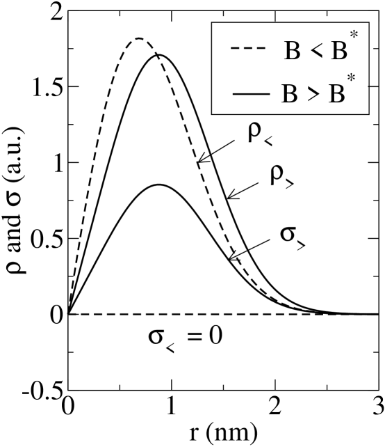
Figure 3: Charge density as a function of the radius $r$. $B<B_{*}$ ($B>B_{*}$) should be understood as $B$ slightly smaller (higher) than $B_{*}$. The charge density $\rho$ is only slightly affected when $B$ goes across $B_{*}$. The spin density $\sigma$ is zero when $B<B_{*}$. It has the profile of the charge density as $B>B_{*}$ ($\sigma_{>}=\frac{1}{2}\rho_{>}$).

The dynamics of the dot between the two macroscopic spin states $S=0,1$ is induced by the coupling to the contacts. Tunneling to and from the dot is only virtual and occupation of the dot, if tuning is appropriate, is still $N=2$. As shown by a Schrieffer-Wolff transformation [14], coupling to the leads involves both orbital and spin variables. However, in the special situation here devised, the exchange of angular momentum is locked in with that of the spin in such a way that coupling is overall of AF type.

This Kondo coupling is peculiar. Of the four levels involved, the two crossing levels play the role of the levels of an effective spin $\frac{1}{2}$, $S_{eff}$, which is acted on by the deviations $\delta B=B-B_{*}$, only. The other two levels can be attributed to another spin $\frac{1}{2}$, $S_{r}$ which is fully decoupled. In the dynamics of $S_{eff}$, the external magnetic field $B_{*}$ disappears completely, provided conduction electrons of both spin orientations are present at $\epsilon_{F}$. If the hybridization with the contacts, $\Delta$, is large enough and $T<T_{K}$, the system flows towards the strongly-coupled fixed point of a standard spin $\frac{1}{2}$ Kondo model, unlike what happens at the TS crossing point. The spin $S_{eff}$ is screened out by the spin density of the delocalized electrons and $S_{r}$ only survives. We end up with charge $N=2$ on the dot and a dot spin $S_{r}=1/2$ with levels splitted in the magnetic field. This is the inverted effect $w.r.to$ Kondo coupling for $N=\>odd$ and leads to fractionalization of the spin in the QD.

3 Summary

To conclude, Kondo conduction in a QD at CB is the striking realization of a macroscopic entangled state between the dot and the contacts. Alternatively, it can be seen as an extreme condition by which the measuring apparatus is fully invasive. Tunneling across the dot is no longer perturbative and separation of the dot total spin from the dot charge sets in. Because of the internal structure of the dot, new properties of the Kondo conduction arise, which are not present in the conductivity of diluted alloys where the Kondo effect was first discovered. In particular, while the presence of a magnetic field, by lifting the degeneracy of the impurity levels is disruptive in diluted alloys, strong Coulomb interaction in dots can give rise to drastic orbital changes and to level crossing. In these conditions the magnetic field acts in favour of a Kondo coupling and strong conduction anomalies in dots at Coulomb blockade can be measured. The Kondo temperature in these systems is rather low ($T_{K}\sim 100mK$ and below ). This notwithstanding, it is the very discreteness of the levels in the confined dot geometry to support the flow to strong coupling at low temperature, irrespective of the influence of the environment.

99

References

- [1] D.Goldhaber-Gordon, H.Shtrikman, D.Mahalu, D.Abusch-Magder, U.Meirav and M.A.Kastner, Nature 391, 156 (1998)
- [2] S.M.Cronenwett,T.H.Oosterkamp and L.P.Kouwenhoven Science 281,540 (1998)
- [3] J.Schmid,JWeis,K.Eberl and K.v.Klitzing, Physica B 256-258,182 (1998)
- [4] L.P. Kouwenhowen et al., in “Mesoscopic electron transport”, NATO ASI Series E 345,105; L.Sohn, L.P.Kouwenhoven and G.Schön eds., Kluwer, Dordrecht,Netherlands (1997); L.P. Kouwenhoven et al. , Science 278, 1788 (1997); S. Tarucha et al., Phys. Rev. Lett. 77, 3613 (1996).
- [5] A.C. Hewson: “The Kondo Effect to Heavy Fermions” (Cambridge University Press, Cambridge, 1993); G.D.Mahan, “Many-Particle Physics” (New York: Plenum Press, 1990).
- [6] J.Kondo, Prog.Theoret. Phys. 32 37 (1964); Solid State Physics, vol. 23, F.Seitz and Turnbull eds, Academic Press, New York, pg.183 (1969)
- [7] L.I.Glazman and M.E.Raikh, Pis’ma Zh.Eksp.Teor.Fiz. 47,378 (1988) [JETP Lett.47, 452 (1988)]; T.K. Ng and P.A.Lee, Phys. Rev. Lett. 61, 1768 (1988); Y.Meir, N.S.Wingreen and P.A.Lee, Phys.Rev.Lett. 70, 2601 (1993)
- [8] P.W.Anderson, Phys.Rev.124, 41 (1961)
- [9] S. Sasaki, S. De Franceschi, J.M. Elzerman, W.G. van der Wiel, M. Eto, S. Tarucha and L.P. Kouwenhoven, Nature 405, 764 (2000).
- [10] S. Tarucha, D.G. Austing, Y. Tokura, W.G. van der Wiel and L.P. Kouwenhoven, Phys. Rev. Lett. 84, 2485 (2000).
- [11] B. Jouault, G. Santoro and A. Tagliacozzo, Phys. Rev. B 61, 10242 (2000).
- [12] M. Eto and Y. Nazarov, Phys.Rev.Lett.85,1306 (2000)
- [13] M. Pustilnik and L.I. Glazman, Phys.Rev.Lett.85,2993 (2000)
- [14] D. Giuliano and A. Tagliacozzo, Phys. Rev. Lett. 84, 4677 (2000); D. Giuliano, B.Jouault and A. Tagliacozzo, cond-mat/0010054 (2000)
- [15] P.W.Anderson, G.Yuval and D.R.Haman Phys.Rev. B11, 4464 (1970)
- [16] D.R.Hamann, Phys.Rev. B2,1373 (1970)
- [17] M.Di Stasio, G.Morandi and A.Tagliacozzo, Phys.Lett. A206 ,211 (1995)
- [18] B.Nienhuis, ”Coulomb Gas Formulation of Two-dimensional Phase Transitions”,C. Domb and J.Lebowitz Eds., (Academic Press) (1987)
- [19] A.M.Tsvelick and P.B.Wiegmann, Advances in Physics 32, 453 (1983); P.B.Wiegmann and A.M.Tsvelick, J.Phys.C,2281 (1983), ibidem, 2321.