Epidemic dynamics and endemic states in complex networks

Abstract

We study by analytical methods and large scale simulations a dynamical model for the spreading of epidemics in complex networks. In networks with exponentially bounded connectivity we recover the usual epidemic behavior with a threshold defining a critical point below which the infection prevalence is null. On the contrary, on a wide range of scale-free networks we observe the absence of an epidemic threshold and its associated critical behavior. This implies that scale-free networks are prone to the spreading and the persistence of infections whatever spreading rate the epidemic agents might possess. These results can help understanding computer virus epidemics and other spreading phenomena on communication and social networks.

I Introduction

Many social, biological, and communication systems can be properly described by complex networks whose nodes represent individuals or organizations and links mimic the interactions among them [1, 2]. Recently, many authors have recognized the importance of local clustering in complex networks. This implies that some special nodes of the network posses a larger probability to develop connections pointing to other nodes. Particularly interesting examples of this kind of behavior are found in metabolic networks [3], food webs [4], and, most importantly, in the Internet and the world-wide-web, where the networking properties have been extensively studied because of their technological and economical relevance [2, 5, 6, 7].

Complex networks can be classified in two main groups, depending on their connectivity properties. The first and most studied one is represented by the exponential networks, in which the nodes’ connectivity distribution (the probability $P(k)$ that a node is connected to other $k$ nodes) is exponentially bounded [8, 9, 10]. The typical example of an exponential network is the random graph model of Erdös and Rényi [9]. A network belonging to this class that has recently attracted a great deal of attention is the Watts and Strogatz model (WS) [10, 11, 12], which has become the prototypical example of a small-world network [13]. A second and very different class of graph is identified by the scale-free (SF) networks which exhibit a power-law connectivity distribution [14],

$$P(k)\sim k^{-2-\gamma},$$ (1)

where the parameter $\gamma$ must be larger than zero to ensure a finite average connectivity $\left<k\right>$. This kind of distribution implies that each node has a statistically significant probability of having a very large number of connections compared to the average connectivity of the network $\left<k\right>$. In particular, we will focus here on the Barabási and Albert model (BA) [14], which results in a connectivity distribution $P(k)\sim k^{-3}$.

In view of the wide occurrence of complex networks in nature, it becomes a very interesting issue to inspect the effect of their complex features on the dynamics of epidemic and disease spreading[15], and more in general on the nonequilibrium phase transitions that usually characterize these type of phenomena [16]. It is easy to foresee that the characterization and understanding of epidemic dynamics on these networks can find immediate applications to a wide range of problems, ranging from computer virus infections [17], epidemiology [18], and the spreading of polluting agents [19].

In this paper, we shall study the susceptible-infected-susceptible (SIS) model [18] on complex networks. We study analytically the prevalence and persistence of infected individuals in exponential and SF networks by using a single-site approximation that takes into account the inhomogeneity due to the connectivity distribution. We find that exponential networks show, as expected, an epidemic threshold (critical point) separating an infected from a healthy phase. The density of infected nodes decreases to zero at the threshold with the linear behavior typical of a mean-field (MF) critical point [16]. The SF networks, on the other hand, show a very different and surprising behavior. For $0<\gamma\leq 1$ the model does not show an epidemic threshold and the infection can always pervade the whole system. In the region $1<\gamma\leq 2$, the model shows an epidemic threshold that is approached, however, with a vanishing slope; i.e. in the absence of critical fluctuations. Only for $\gamma>2$ we recover again the usual critical behavior at the threshold. In these systems, because of the nonlocal connectivity, single site approximation predictions are expected to correctly depict the model’s behavior. In order to test our predictions, we perform large scale numerical simulations on both exponential and SF networks. Numerical results are in perfect agreement with the analytical predictions and confirm the overall picture for the SIS model on complex networks given by the theoretical analysis. The striking absence of an epidemic threshold on SF networks, a characteristic element in mathematical epidemiology, radically changes many of the conclusions drawn in classic epidemic modeling. The present results could be relevant also in the field of absorbing-phase transitions and catalytic reactions in which the spatial interaction of the reactants can be modeled by a complex network [16].

The paper is organized as follows. In Sec. II we introduce the SIS model in a general context. Sec. III is devoted to the analysis of exponentially bounded networks, exemplified by the WS model. In Sec. IV we analyze the scale-free BA model, with connectivity $P(k)\sim k^{-3}$. Sec. V extends the analytical approach applied to the BA model to generalized SF networks, with connectivity distribution $P(k)\sim k^{-2-\gamma}$, $\gamma>0$. Finally, in Sec. VI we draw our conclusions and perspectives.

II The SIS model

To address the effect of the topology of complex networks in epidemic spreading we shall study the standard susceptible-infected-susceptible (SIS) epidemiological model [18]. Each node of the network represents an individual and each link is a connection along which the infection can spread to other individuals. The SIS model relies on a coarse grained description of the individuals in the population. Within this description, individuals can only exist in two discrete states, namely, susceptible, or “healthy”, and infected. These states completely neglect the details of the infection mechanism within each individual. The disease transmission is also described in an effective way. At each time step, each susceptible node is infected with probability $\nu$ if it is connected to one or more infected nodes. At the same time, infected nodes are cured and become again susceptible with probability $\delta$, defining an effective spreading rate $\lambda=\nu/\delta$. (Without lack of generality, we set $\delta=1$.) Individuals run stochastically through the cycle susceptible $\to$ infected $\to$ susceptible, hence the name of the model. The updating can be performed with both parallel or sequential dynamics[16]. The SIS model does not take into account the possibility of individuals removal due to death or acquired immunization[18]. It is mainly used as a paradigmatic model for the study of infectious disease that leads to an endemic state with a stationary and constant value for the prevalence of infected individuals, i.e., the degree to which the infection is widespread in the population.

The topology of the network that specifies the interactions among individuals is of primary importance in determining many of the model’s features. In standard topologies the most significant result is the general prediction of a nonzero epidemic threshold $\lambda_{c}$ [18]. If the value of $\lambda$ is above the threshold, $\lambda\geq\lambda_{c}$, the infection spreads and becomes persistent in time. Below it, $\lambda<\lambda_{c}$, the infection dies out exponentially fast. In both sides of the phase diagram it is possible to study the behavior in time of interesting dynamical magnitudes of epidemics, such as the time survival probability and the relaxation to the healthy state or the stationary endemic state. In the latter case, if we start from a localized seed we can study the epidemic outbreak preceding the endemic stabilization. From this general picture, it is natural to consider the epidemic threshold as completely equivalent to a critical point in a nonequilibrium phase transition [16]. In this case, the critical point separates an active phase with a stationary density of infected nodes (an endemic state) from an absorbing phase with only healthy nodes and null activity. In particular, it is easy to recognize that the SIS model is a generalization of the contact process (CP) model, that has been extensively studied in the context of absorbing-state phase transitions[16].

In order to obtain an analytical understanding of the SIS model behavior on complex networks, we can apply a single site dynamical MF approach, that we expect to recover exactly the model’s behavior due to the nonlocal connectivity of these graphs. Let us consider separately the case of the exponentially bounded and SF networks.

III Exponential networks: the Watts-Strogatz model

The class of exponential networks refers to random graph models which produce a connectivity distribution $P(k)$ peaked at an average value $\left<k\right>$ and decaying exponentially fast for $k\gg\left<k\right>$ and $k\ll\left<k\right>$. Typical examples of such a network are the random graph model[9] and the small-world model of Watts and Strogatz (WS) [10]. The latter has recently been the object of several studies as a good candidate for the modeling of many realistic situations in the context of social and natural networks. In particular, the WS model shows the “small-world” property common in random graphs [13]; i.e., the diameter of the graph— the shortest chain of links connecting any two vertices—increases very slowly, in general logarithmically with the network size [12]. On the other hand, the WS model has also a local structure (clustering property) that is not found in random graphs with finite connectivity[10, 12]. The WS graph is defined as follows [10, 12]: The starting point is a ring with $N$ nodes, in which each node is symmetrically connected with its $2K$ nearest neighbors. Then, for every node each link connected to a clockwise neighbor is rewired to a randomly chosen node with probability $p$, and preserved with probability $1-p$. This procedure generates a random graph with a connectivity distributed exponentially for large $k$ [10, 12], and an average connectivity $\left<k\right>=2K$. The graphs has small-world properties and a non-trivial “clustering coefficient”; i.e., neighboring nodes share many common neighbors [10, 12]. The richness of this model has stimulated an intense activity aimed at understanding the network’s properties upon changing $p$ and the network size $N$ [10, 11, 12, 13, 20, 21]. At the same time, the behavior of physical models on WS graphs has been investigated, including epidemiological percolation models[15, 20, 22] and models with epidemic cycles[23].

Here we focus on the WS model with $p=1$; it is worth noticing that even in this extreme case the network retains some memory of the generating procedure. The network, in fact, is not locally equivalent to a random graph in that each node has at least $K$ neighbors. Since the fluctuations in the connectivity are very small in the WS graph, due to its exponential distribution, we can approach the analytical study of the SIS model by considering a single MF reaction equation for the density of infected nodes $\rho(t)$:

$$\partial_{t}\rho(t)=-\rho(t)+\lambda\left<k\right>\rho(t)\left[1-\rho(t)\right]+h.o.~{}.$$ (2)

The MF character of this equation stems from the fact that we have neglected the density correlations among the different nodes, independently of their respective connectivities. In Eq. (2) we have ignored all higher order corrections in $\rho(t)$, since we are interested in the onset of the infection close to the phase transition; i.e., at $\rho(t)\ll 1$. The first term on the r.h.s. in Eq. (2) considers infected nodes become healthy with unit rate. The second term represents the average density of newly infected nodes generated by each active node. This is proportional to the infection spreading rate $\lambda$, the number of links emanating from each node, and the probability that a given link points to a healthy node, $\left[1-\rho(t)\right]$. In these models, connectivity has only exponentially small fluctuations ($\left<k^{2}\right>\sim\left<k\right>$) and as a first approximation we have considered that each node has the same number of links, $k\simeq\left<k\right>$. This is equivalent to an homogeneity assumption for the system’s connectivity. After imposing the stationarity condition $\partial_{t}\rho(t)=0$, we obtain the equation

$$\rho\left[-1+\lambda\left<k\right>(1-\rho)\right]=0$$ (3)

for the steady state density $\rho$ of infected nodes. This equation defines an epidemic threshold $\lambda_{c}=\left<k\right>^{-1}$, and yields:

$$\rho = 0\;\qquad\qquad\mbox{\rm if $\lambda<\lambda_{c}$},$$ (5)

$$\rho \sim \lambda-\lambda_{c}\qquad\mbox{\rm if $\lambda>\lambda_{c}$}.$$ (6)

In analogy with critical phenomena, we can consider $\rho$ as the order parameter of a phase transition and $\lambda$ as the tuning parameter, recovering a MF critical behavior [24]. It is possible to refine the above calculations by introducing connectivity fluctuations (as it will be done later for SF networks, see Sec. IV). However, the results are qualitatively and quantitatively the same as far as we are only concerned with the model’s behavior close to the threshold.

In order to compare with the analytical prediction we have performed large scale simulations of the SIS model in the WS network with $p=1$. Simulations were implemented on graphs with number of nodes ranging from $N=10^{3}$ to $N=3\times 10^{6}$, analyzing the stationary properties of the density of infected nodes $\rho$; i.e. the infection prevalence. Initially we infect half of the nodes in the network, and iterate the rules of the SIS model with parallel updating. In the active phase, after an initial transient regime, the systems stabilize in a steady state with a constant average density of infected nodes. The prevalence is computed averaging over at least $100$ different starting configurations, performed on at least $10$ different realization of the random networks. In our simulations we consider the WS network with parameter $K=3$, which corresponds to an average connectivity $\left<k\right>=6$.

FIG. 1.: Density of infected nodes $\rho$ as a function of $\lambda$ in the WS network (full line) and the BA network (dashed line).

FIG. 2.: Log-log plot of density of infected node $\rho$ as a function of $\lambda-\lambda_{c}$ in WS network, with $\lambda_{c}=0.1643\pm 0.01$. The full line is a fit to the form $\rho\sim(\lambda-\lambda_{c})^{\beta}$, with an exponent $\beta=0.97\pm 0.04$.

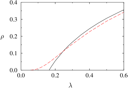
As shown in Figs. 1 and 2, the SIS model on a WS graph exhibits an epidemic threshold $\lambda_{c}=0.1643\pm 0.01$ that is approached with linear behavior by $\rho$. The value of the threshold is in good agreement with the MF predictions $\lambda_{c}=1/2K=0.1666$, as well as the density of infected nodes behavior. In Fig. 2 we plot $\rho$ as a function of $\lambda-\lambda_{c}$ in log-log scale. A linear fit to the form $\rho\sim(\lambda-\lambda_{c})^{\beta}$ provides an exponent $\beta=0.97\pm 0.04$, in good agreement with the analytical finding of the Eq. (6).

FIG. 3.: Density of infected nodes $\rho(t)$ as a function of time in supercritical spreading experiments in the WS network. Network size $N=1.5\times 10^{6}$. Spreading rates range from $\lambda-\lambda_{c}=0.002$ to $0.0007$ (top to bottom).

FIG. 4.: Density of infected nodes $\rho(t)$ as a function of time in subcritical spreading experiments in the WS network. Network size $N=3\times 10^{6}$. Spreading rates range from $\lambda_{c}-\lambda=0.005$ to $0.03$ (right to left).

FIG. 5.: Surviving probability $P_{s}(t)$ as a function of time in subcritical spreading experiments in the WS network. Network size $N=3\times 10^{6}$. Spreading rates range from $\lambda_{c}-\lambda=0.005$ to $0.03$ (right to left). Inset: Surviving probability for a fixed spreading rate $\lambda_{c}-\lambda=0.005$ and network sizes $N=3\times 10^{5}$, $10^{6}$, and $3\times 10^{6}$.

FIG. 6.: Inverse relaxation time for the SIS model in the WS graph as a function of the spreading rate $\lambda$, estimated from the slope of the exponential decay of the infected nodes density $\rho(t)$ ($\circ$) and the survival probability $P_{s}(t)$ ($\Diamond$).

To complete our study of the SIS model in the WS network, we have also analyzed the epidemic spreading properties, computed by considering the time evolution of infections starting from a very small concentration of infected nodes. In Fig. 3 we plot the evolution of the infected nodes density as a function of time for epidemics in the supercritical regime ($\lambda>\lambda_{c}$) which start from a single infected node. Each curve represents the average over several spreading events with the same $\lambda$. We clearly notice a spreading growth faster than any power-law, in agreement with Eq. (2) which predicts an exponential saturation to the endemic steady state. In the subcritical regime ($\lambda<\lambda_{c}$), by introducing a small perturbation to the stationary state $\rho=0$, and keeping only first order terms in Eq. (2), we obtain that the infection decays following the exponential relaxation $\partial_{t}\rho(t)=-\left<k\right>(\lambda_{c}-\lambda)\rho(t)$. This equation introduces a characteristic relaxation time

$$\tau^{-1}=\left<k\right>(\lambda_{c}-\lambda),$$ (7)

that diverges at the epidemic threshold. Below the threshold, the epidemic outbreak dies within a finite time; i.e. it does not reach a stationary endemic state. In Fig. 4 we plot the average of $\rho(t)$ for epidemics starting with an initial concentration $\rho_{0}=0.01$ of infected nodes; the Figure shows a clear exponential approach to the healthy (absorbing) state as predicted by Eq. (7). In the subcritical regime, we can compute also the surviving probability, $P_{s}(t)$, defined as the probability that an epidemic outbreak survives up to the time $t$ [16]. In Fig. 5 we plot the survival probability computed from simulations starting with a single infected node in a WS graph of size $N=3\times 10^{6}$. The survival probability decay is obviously governed by the same exponential behavior and characteristic time of the density of infected nodes as confirmed by numerical simulations. Indeed, below the epidemic threshold, the relaxation to the absorbing state does not depend on the network size $N$ (see inset in Fig. 5), and the average lifetime corresponding to each spreading rate $\lambda$ can be measured by the slope of the exponential tail of $P_{s}(t)$ and $\rho(t)$. By plotting $\tau^{-1}$ as a function of $\lambda_{c}-\lambda$ (see Fig. 6), we recover the analytic predictions ; i.e. the linear behavior and the unique characteristic time for both the density and survival probability decay. The slope of the graph, measured by means of a least squares fitting, provides a value of $6.3$, whereas the intercept yields $1.0$, in good agreement with the theoretical predictions of Eq. (7), $\left<k\right>=6$ and $\left<k\right>\lambda_{c}=1$, respectively.

In summary, numerical and analytical results confirms that for WS graphs, the standard epidemiological picture (often called the deterministic approximation) is qualitatively and quantitatively correct. This result, that is well-known for random graphs, holds also in the WS model despite the different local structure.

IV Scale-free networks: the Barabási-Albert model

The Barabási-Albert (BA) graph was introduced as a model of growing network (such as the Internet or the world-wide-web) in which the successively added nodes establish links with higher probability pointing to already highly connected nodes [14]. This is a rather intuitive phenomenon on the Internet and other social networks, in which new individuals tend to develop more easily connections with individuals which are already well-known and widely connected. The BA graph is constructed using the following algorithm [14]: We start from a small number $m_{0}$ of disconnected nodes; every time step a new vertex is added, with $m$ links that are connected to an old node $i$ with probability

$$\Pi(k_{i})=\frac{k_{i}}{\sum_{j}k_{j}},$$ (8)

where $k_{i}$ is the connectivity of the $i$-th node. After iterating this scheme a sufficient number of times, we obtain a network composed by $N$ nodes with connectivity distribution $P(k)\sim k^{-3}$ and average connectivity $\left<k\right>=2m$ (in this work we will consider the parameters $m_{0}=5$ and $m=3$). Despite the well-defined average connectivity, the scale invariant properties of the network turns out to play a major role on the properties of models such as percolation[22, 25], used to mimic the resilience to attacks of a network. For this class of graphs, in fact, the absence of a characteristic scale for the connectivity makes highly connected nodes statistically significant, and induces strong fluctuations in the connectivity distribution which cannot be neglected. In order to take into account these fluctuations, we have to relax the homogeneity assumption used for exponential networks, and consider the relative density $\rho_{k}(t)$ of infected nodes with given connectivity $k$; i.e., the probability that a node with $k$ links is infected. The dynamical MF reaction rate equations can thus be written as

$$\partial_{t}\rho_{k}(t)=-\rho_{k}(t)+\lambda k\left[1-\rho_{k}(t)\right]\Theta(\rho(t)),$$ (9)

where also in this case we have considered a unitary recovery rate and neglected higher order terms ($\rho(t)\ll 1$). The creation term considers the probability that a node with $k$ links is healthy $[1-\rho_{k}(t)]$ and gets the infection via a connected node. The probability of this last event is proportional to the infection rate $\lambda$, the number of connections $k$, and the probability $\Theta(\rho(t))$ that any given link points to an infected node. We make the assumption that $\Theta$ is a function of the total density of infected nodes $\rho(t)$ [26]. In the steady (endemic) state, $\rho$ is just a function of $\lambda$. Thus, the probability $\Theta$ becomes also an implicit function of the spreading rate, and by imposing stationarity [$\partial_{t}\rho_{k}(t)=0$], we obtain

$$\rho_{k}=\frac{k\lambda\Theta(\lambda)}{1+k\lambda\Theta(\lambda)}.$$ (10)

This set of equations show that the higher the node connectivity, the higher the probability to be in an infected state. This inhomogeneity must be taken into account in the computation of $\Theta(\lambda)$. Indeed, the probability that a link points to a node with $s$ links is proportional to $sP(s)$. In other words, a randomly chosen link is more likely to be connected to an infected node with high connectivity, yielding the relation

$$\Theta(\lambda)=\sum_{k}\frac{kP(k)\rho_{k}}{\sum_{s}sP(s)}.$$ (11)

Since $\rho_{k}$ is on its turn a function of $\Theta(\lambda)$, we obtain a self-consistency equation that allows to find $\Theta(\lambda)$ and an explicit form for Eq. (10). Finally, we can evaluate the order parameter (persistence) $\rho$ using the relation

$$\rho=\sum_{k}P(k)\rho_{k},$$ (12)

In order to perform an explicit calculation for the BA model, we use a continuous $k$ approximation that allows the practical substitution of series with integrals[14]. The full connectivity distribution is given by $P(k)=2m^{2}/k^{-3}$, where $m$ is the minimum number of connection at each node. By noticing that the average connectivity is $\left<k\right>=\int_{m}^{\infty}kP(k)dk=2m$, Eq. (11) gives

$$\Theta(\lambda)=m\lambda\Theta(\lambda)\int_{m}^{\infty}\frac{1}{k^{3}}\frac{k^{2}}{1+k\lambda\Theta(\lambda)},$$ (13)

which yields the solution

$$\Theta(\lambda)=\frac{e^{-1/m\lambda}}{\lambda m}(1-e^{-1/m\lambda})^{-1}.$$ (14)

In order to find the behavior of the density of infected nodes we have to solve Eq. (12), that reads as

$$\rho=2m^{2}\lambda\Theta(\lambda)\int_{m}^{\infty}\frac{1}{k^{3}}\frac{k}{1+k\lambda\Theta(\lambda)}.$$ (15)

By substituting the obtained expression for $\Theta(\lambda)$ and solving the integral we find at the lowest order in $\lambda$

$$\rho\sim e^{-1/m\lambda}$$ (16)

This result shows the surprising absence of any epidemic threshold or critical point in the model; i.e., $\lambda_{c}=0$. This can be intuitively understood by noticing that for usual lattices and MF models, the higher the node’s connectivity, the smaller the epidemic threshold. In the BA network the unbounded fluctuations in the number of links emanating from each node ($\left<k^{2}\right>=\infty$) plays the role of an infinite connectivity, annulling thus the threshold. This implies that infections can pervade a BA network, whatever the infection rate they have.

FIG. 7.: Persistence $\rho$ as a function of $1/\lambda$ for BA networks of different sizes: $N=10^{5}$ ($+$), $N=5\times 10^{5}$ ($\Box$), $N=10^{6}$ ($\times$), $N=5\times 10^{6}$ ($\circ$), and $N=8.5\times 10^{6}$ ($\Diamond$). The linear behavior on the semi-logarithmic scale proves the stretched exponential behavior predicted for the persistence. The full line is a fit to the form $\rho\sim\exp(-C/\lambda)$.

FIG. 8.: The density $\rho_{k}$, defined as the fraction of nodes with connectivity $k$ which are infected, in a BA network of size $N=5\times 10^{5}$ and spreading rates $\lambda=0.1$, $0.08$ and $0.065$ (bottom to top). The plot recovers the form predicted in Eq.(10).

The numerical simulations performed on the BA network confirm the picture extracted from the analytic treatment. We consider the SIS model on BA networks of size ranging from $N=10^{3}$ to $N=8.5\times 10^{6}$. In Fig. 1 we have plotted the epidemic persistence $\rho$ as a function of $\lambda$ in a linear scale. The function $\rho$ approaches smoothly the value $\lambda=0$ with vanishing slope. Fig. 7, in fact, shows that the infection prevalence in the steady state decays with $\lambda$ as $\rho\sim\exp(-C/\lambda)$, where $C$ is a constant. The numerical value obtained $C^{-1}=2.5$ is also in good agreement with the theoretical prediction $C^{-1}=m=3$. In order to rule out the presence of finite size effect hiding an abrupt transition (the so-called smoothing out of critical points[16]), we have inspected the behavior of the stationary persistence for network sizes varying over three orders of magnitude. The total absence of scaling of $\rho$ and the perfect agreement for any size with the analytically predicted exponential behavior allows us to definitely confirm the absence of any finite epidemic threshold. In Fig. 8, we also provide an illustration of the behavior of the probability $\rho_{k}$ that a node with given connectivity $k$ is infected. Also in this case we found a behavior with $k$ in complete agreement with the analytical prediction of Eq. (10).

FIG. 9.: Density of infected nodes $\rho(t)$ as a function of time in supercritical spreading experiments in the BA network. Network size $N=10^{6}$. Spreading rates range from $\lambda=0.05$ to $0.065$ (bottom to top).

FIG. 10.: Surviving probability $P_{s}(t)$ as a function of time in subcritical spreading experiments in the BA network. Spreading rate $\lambda=0.065$. Network sizes ranging from $N=6.25\times 10^{3}$ to $N=5\times 10^{5}$ (bottom to top).

Our numerical study of the spreading dynamical properties on the BA network is reported in Figs. 9 and 10. In Fig. 9 we plot the growth of the epidemics starting from a single infected node. We observe that the spreading growth in time has an algebraic form, as opposed to the exponential growth typical of mean-field continuous phase transitions close to the critical point [16], and the behavior of the SIS model in the WS graph (see Fig. 3). The surviving probability $P_{s}(t)$ for a fixed value of $\lambda$ and networks of different size $N$ is reported in Fig 10. In this case, we recover an exponential behavior in time, that has its origin in the finite size of the network. In fact, for any finite system, the epidemic will eventually die out because there is a finite probability that all individuals cure the infection at the same time. This probability is decreasing with the system size and the lifetime is infinite only in the thermodynamic limit $N\to\infty$. However, the lifetime becomes virtually infinite (the metastable state has a lifetime too long for our observation period) for enough large sizes that depend upon the spreading rate $\lambda$. This is a well-known feature of the survival probability in finite size absorbing-state systems poised above the critical point. In our case, this picture is confirmed by numerical simulations that shows that the average lifetime of the survival probability is increasing with the network size for all the values of $\lambda$. Given the intrinsic dynamical nature of scale-free networks, this result could possibly have several practical implications in the study of epidemic spreading in real growing networks.

The numerical analysis supports and confirms the analytical results pointing out the existence of a different epidemiological framework for SF networks. The absence of an epidemic threshold, a central element in the theory of epidemics, opens a different scenario and rationalization for epidemic events in these networks. The dangerous absence of the epidemic threshold, that leaves SF networks completely disarmed with respect to epidemic outbreaks, is fortunately balanced from a corresponding exponentially low prevalence at small spreading rates. In addition, the absence of a critical threshold, and the associated diverging response function, makes the increase of the endemic prevalence with the spreading rate very slow. This new perspective seems to be particularly relevant in the rationalization of epidemic data from computer virus infections[27].

V Generalized scale-free networks

Recently there has been a burst of activity in the modeling of SF complex network. The recipe of Barabási and Albert[14] has been followed by several variations and generalizations [28, 29, 30, 31] and the revamping of previous mathematical works[32]. All these studies propose methods to generate SF networks with variable exponent $\gamma$. The analytical treatment presented in the previous section for the SIS model can be easily generalized to SF networks with connectivity distribution with $\gamma>0$. Consider a generalized SF network with a normalized connectivity distribution given by

$$P(k)=(1+\gamma)m^{1+\gamma}k^{-2-\gamma},$$ (17)

where we are approximating the connectivity $k$ as a continuous variable and assuming $m$ the minimum connectivity of any node. The average connectivity is thus

$$\left<k\right>=\int_{m}^{\infty}kP(k)dk=\frac{1+\gamma}{\gamma}m.$$ (18)

For any connectivity distribution, the relative density of infected nodes $\rho_{k}$ is given by Eq. (10). Applying then Eq. (11) to compute self-consistently the probability $\Theta$, we obtain

$$\Theta(\lambda)=F[1,\gamma,1+\gamma,-(m\lambda\Theta(\lambda))^{-1}],$$ (19)

where $F$ is the Gauss hypergeometric function [33]. On the other hand, the expression for the density $\rho$, Eq. (12), yields

$$\rho=F[1,1+\gamma,2+\gamma,-(m\lambda\Theta(\lambda))^{-1}].$$ (20)

In order to solve Eqs. (19) and (20) in the limit $\rho\to 0$ (which obviously corresponds also to $\Theta\to 0$, we must perform a Taylor expansion of the hypergeometric function. The expansion for Eq. (19) has the form [33]

$$F[1,\gamma,1+\gamma,-(m\lambda\Theta(\lambda))^{-1}]$$ (21)

$$\simeq \frac{\gamma\pi}{\sin(\gamma\pi)}(m\lambda\Theta)^{\gamma}+\gamma\sum_{n=1}^{\infty}(-1)^{n}\frac{(m\lambda\Theta)^{n}}{n-\gamma},$$ (22)

where $\Gamma(x)$ is the standard gamma function. An analogous expression holds for (20). The expansion (22) is valid for any $\gamma\neq 1,2,3,\ldots$. Integer values of $\gamma$ must be analyzed in a case by case basis. (The particular value $\gamma=1$ was considered in the previous Section.) For all values of $\gamma$, the leading behavior of Eq. (20) is the same:

$$\rho\simeq\frac{1+\gamma}{\gamma}m\lambda\Theta$$ (23)

The leading behavior in the r.h.s. of Eq. (22), on the other hand, depends of the particular value of $\gamma$:

(i) $0<\gamma<1$: In this case, one has

$$\Theta(\lambda)\simeq\frac{\gamma\pi}{\sin(\gamma\pi)}(m\lambda\Theta)^{\gamma},$$ (24)

from which we obtain

$$\Theta(\lambda)\simeq\left[\frac{\gamma\pi}{\sin(\gamma\pi)}\right]^{1/(1-\gamma)}\left(m\lambda\right)^{\gamma/(1-\gamma)}.$$ (25)

Combining this with Eq. (23), we obtain:

$$\rho\sim\lambda^{1/(1-\gamma)}.$$ (26)

Here we have again the total absence of any epidemic threshold and the associated critical behavior, as we have already shown for the case $\gamma=1$. In this case, however, the relation between $\rho$ and $\lambda$ is given by a power law with exponent $\beta=1/(1-\gamma)$; i.e., $\beta>1$.

(ii) $1<\gamma<2$: In this case, to obtain a nontrivial information for $\Theta$, we must keep the first two most relevant terms in Eq. (22):

$$\Theta(\lambda)\simeq\frac{\gamma\pi}{\sin(\gamma\pi)}(m\lambda\Theta)^{\gamma}+\frac{\gamma}{\gamma-1}m\lambda\Theta.$$ (27)

From here we get:

$$\Theta(\lambda)\simeq\left[\frac{-\sin(\gamma\pi)}{\pi(\gamma-1)}\frac{m}{(m\lambda)^{\gamma}}\left(\lambda-\frac{\gamma-1}{m\gamma}\right)\right]^{1/(\gamma-1)}.$$ (28)

The expression for $\rho$ is finally:

$$\rho\simeq\left(\lambda-\frac{\gamma-1}{m\gamma}\right)^{1/(\gamma-1)}\sim\left(\lambda-\lambda_{c}\right)^{1/(\gamma-1)}.$$ (29)

That is, we obtain a power-law behavior with exponent $\beta=1/(\gamma-1)>1$, but now we observe the presence of a nonzero threshold

$$\lambda_{c}=\frac{\gamma-1}{m\gamma}.$$ (30)

In this case, a critical threshold reappears in the model. However, the epidemic threshold is approached smoothly without any sign of the singular behavior associated to critical point.

(iii) $\gamma>2$: The relevant terms in the $\Theta$ expansion are now

$$\Theta(\lambda)\simeq\frac{\gamma}{\gamma-1}m\lambda\Theta-\frac{\gamma}{\gamma-2}(m\lambda\Theta)^{2},$$ (31)

and the relevant expression for $\Theta$ is

$$\Theta(\lambda)\simeq\frac{\gamma-2}{\gamma-1}\frac{1}{\lambda^{2}m}\left(\lambda-\frac{\gamma-1}{m\gamma}\right)$$ (32)

which yields the behavior for $\rho$

$$\rho\sim\lambda-\lambda_{c}$$ (33)

with the same threshold $\lambda_{c}$ as in Eq. (30) and an exponent $\beta=1$. In other words, we recover the usual critical framework in networks with connectivity distribution that decays faster than $k$ to the fourth power. Obviously, an exponentially bounded network is included in this last case, recovering the results obtained with the homogeneous approximation of Sec. III.

In summary, for all SF networks with $0<\gamma\leq 1$, we recover the absence of an epidemic threshold and critical behavior; i.e. $\rho=0$ only if $\lambda=0$, and $\rho$ has a vanishing slope when $\lambda\to 0$. In the interval $1<\gamma<2$, an epidemic threshold reappears ($\rho\to 0$ if $\lambda\to\lambda_{c}$), but it is also approached with vanishing slope; i.e. no singular behavior. Eventually, for $\gamma>2$ the usual MF critical behavior is recovered and the SF network is indistinguishable from an exponential network.

VI Conclusions

The emerging picture for disease spreading in complex networks emphasizes the role of topology in epidemic modeling. In particular, the absence of epidemic threshold and critical behavior in a wide range of SF networks provides an unexpected result that changes radically many standard conclusions on epidemic spreading. Our results indicate that infections can proliferate on these networks whatever spreading rates they may have. These very bad news are, however, balanced by the exponentially small prevalence for a wide range of spreading rates ($\lambda\ll 1$). This point appears to be particularly relevant in the case of technological networks such as the Internet and the world-wide-web that show a SF connectivity with exponents $\gamma\simeq 2.5$ [5, 6]. For instance, the present picture fits perfectly with the observation from real data of computer virus spreading, and could solve the longstanding problem of the generalized low prevalence of computer viruses without assuming any global tuning of the spreading rates[17, 27]. The peculiar properties of SF networks also open the path to many other questions concerning the effect of immunity and other modifications of epidemic models. As well, the critical properties of many nonequilibrium systems could be affected by the topology of SF networks. Given the wide context in which SF networks appears, the results obtained here could have intriguing implications in many biology and social systems.