Monte Carlo Dynamics of driven Flux Lines in Disordered Media

Abstract

We show that the common local Monte Carlo rules used to simulate the motion of driven flux lines in disordered media cannot capture the interplay between elasticity and disorder which lies at the heart of these systems. We therefore discuss a class of generalized Monte Carlo algorithms where an arbitrary number of line elements may move at the same time. We prove that all these dynamical rules have the same value of the critical force and possess phase spaces made up of a single ergodic component. A variant Monte Carlo algorithm allows to compute the critical force of a sample in a single pass through the system. We establish dynamical scaling properties and obtain precise values for the critical force, which is finite even for an unbounded distribution of the disorder. Extensions to higher dimensions are outlined.

In the last few years, the study of elastic manifolds in random media has retained much attention.

These systems appear in a wide range of physical systems, ranging from vortices in type-II superconductors [1], to charge density waves [2], interfaces in disordered magnets [3], and to the problem of directed polymer growth [4]. The response of elastic manifolds to an external driving force $f$ is highly non-trivial: at temperature $T=0$, the manifold is completely “pinned” at small forces, while it moves with non-zero velocity at forces larger than a certain critical force $f_{c}$. At finite, but small, $T$, a socalled “creep motion” takes place for $f\ll f_{c}$, while the motion at $f\gg f_{c}$ is described by viscous flow. Many details of this dynamical problem, both at $T=0$ and at finite temperatures, have yet to be understood fully [5, 6].

This paper is concerned with an analysis of the dynamical Monte Carlo method [7] as applied to lattice models of driven elastic manifolds in random media. We argue that the common local Monte Carlo rules [8, 9, 10, 11] are incompatible with the Langevin dynamics [12, 13, 14] which defines time evolution in continuum models. We instead propose generalized Monte Carlo algorithms where an arbitrary number of elements may move at the same time. For this class of algorithms, we can establish the uniqueness of the critical force and simple connectedness of phase space. Furthermore, we devise a method which simplifies enormously the calculation of the critical force.

Our model is sketched in figure 1. We consider a flux line $x^{t}=\{x_{i}^{t}\}_{i=0,\ldots,L}$ moving at times $t=0,1,2,\ldots$ on a spatial square lattice with a random potential $V(i,x)$ with $x=0,1,\ldots$. Mainly for convenience (cf below), we also introduce a metric constraint

$$|x_{i+1}^{t}-x_{i}^{t}|\leq 1$$ (1)

as well as periodic boundary conditions ($x_{0}^{t}=x_{L}^{t}$) on the flux line. The random potential satisfies

$$V(i,x_{i}+M)=V(i+L,x_{i})=V(i,x_{i}).$$ (2)

This condition defines an effective sample of size $(L,M)$. While eq.(2) is essential for the following, the periodic boundary condition for the flux line and the specific choice of lattice are inessential details.

The energy of a flux line $x^{t}$ in presence of an external driving force $f$ is given by

$$E(x^{t})=\sum_{i=1}^{L}V(i,x_{i}^{t})-fx_{i}^{t}+\frac{c}{2}(x_{i+1}^{t}-x_{i}^{t})^{2},$$ (3)

where $c$ is an elastic constant.

FIG. 1.: Flux line $x^{t}=\{x_{i}^{t}\}_{i=0,\ldots,L}$ on a spatial square lattice with disorder potential $V(i,x)$. Periodic boundary conditions in $i$ and $x$ are assumed for the lattice and the disorder, respectively. The direction of the driving force $f$ is indicated, as well as a proposed local Monte Carlo move. The local dynamics lead to a trivial critical force in the limit of large systems.

In figure 1, a local Monte Carlo move is indicated. In the local Monte Carlo algorithm, the proposed configuration $\tilde{x}$ differs from the present configuration $x^{t}$ only on a random position $i$. One chooses $\tilde{x_{i}}=x_{i}\pm 1$ with equal probability. At zero temperature, the move is accepted ($x^{t+1}=\tilde{x}$) if the energy eq.(3) decreases and if the metric constraint eq.(1) is satisfied. Otherwise, it is rejected ($x^{t+1}=x^{t}$).

This rule has been used in past simulations, in spite of its very serious shortcomings. Consider, for example, the site in figure 1 marked with a circle, $(i_{0},x_{0})$. The flux line $x^{t}$ shown in figure 1 can only move away from $(i_{0},x_{0})$ if $f>V(i_{0},x_{0}+1)-V(i_{0},x_{0})+c$. Even an infinitely long flux line $(L\rightarrow\infty)$ is thus stopped by a single deep pin $V(i_{0},x_{0})$ and the motion does not differ qualitatively from the one of a point in a disordered potential [15, 16]. For an unbounded distribution of $V$, the critical force is always infinite, exposing clearly the pathology of the local Monte Carlo algorithm.

Some authors have therefore used a bounded distribution, $V<V_{\max}$. However, it is easy to see that in this case the local Monte Carlo algorithm does not correctly incorporate the disorder, and the flux line’s motion is trivial: in the limit of large system size $LM\gg 1$, the flux line will be free to move if $f>2V_{\max}$, in a way which will be similar to the motion of the non-disordered system. This has already been pointed out for the analogous case of the random Ising model [9].

We conclude that the description of a driven flux line by means of a local Monte Carlo algorithm or its variants [11] eliminates the very feature which makes the problem interesting in the first place, namely the competition between elasticity and disorder. This competition is preserved in the continuum Langevin dynamics [13, 5].

Within the Monte Carlo method, we are thus naturally lead to consider generalizations of the model. It can be seen easily that the problem just discussed persists even if we abandon the metric constraint eq.(1). The only remaining option is therefore to abandon the local moves in favor of rules which allow global moves. The study of global moves in dynamical Monte Carlo is the subject of this paper.

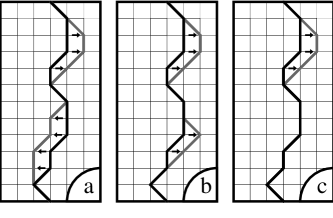
FIG. 2.: Non-local Monte Carlo moves which are considered in this paper. Model $a$: all positions $x_{i}^{t}$ ($i=1,L$) may change at the same time by a value $\pm 1$. Model $b$: as in $a$, but the motion is either in forward or in backward direction. Model $c$: as in $b$, but the motion is restricted to single ‘fronts’.

Let us define “Model $a$” dynamics by a proposed move $x^{t}\rightarrow x^{t}+\delta^{t}$ with $\delta^{t}=\{\delta_{i}^{t}\}_{i=0,\ldots,L}$ such that

$$\delta_{i}=\left\{\begin{array}[]{ccc}+1&&p\\ 0&\mbox{ with prob.}&1-2p\\ -1&&p\end{array}\right\}\;\;\;\forall i\;\;\;\mbox{(Model $a$)}$$ (4)

At zero temperature, the proposed move is accepted, $x^{t+1}=x^{t}+\delta$, if the resulting configuration both satisfies the metric constraint eq.(1) and decreases the string energy eq.(3). Note that under Model $a$ dynamics a move is proposed with the same probability as its inverse. This serves to enforce detailed balance, which allows to naturally extend the rule to finite temperatures via the Metropolis algorithm. The same can usually not be done for cellular automata methods [13, 14, 17].

A possible second rule (“Model $b$”) chooses at each time $t$ with equal probability either to move forward ($\mu^{t}=1$) or backwards ($\mu^{t}=-1$). The following move is then proposed:

$$\delta_{i}=\left\{\begin{array}[]{ccc}\mu^{t}&&p\\ &\mbox{ with prob.}&\\ 0&&1-p\\ \end{array}\right\}\;\;\;\forall i\;\;\;\mbox{(Model $b$)}$$ (5)

The simulation of dynamical models with such global moves may appear hopeless because of the difficulty to detect the few energetically favorable choices among the exponential number of possibilities in eq.(4) or in eq.(5).

To show that the situation is much less desperate, let us first define a ‘forward front’ of length $k$ as a contiguous set of points $i,i+1,....,i+k-1$ which may advance together without violating the metric constraints eq.(1) ($\delta_{i}=\delta_{i+1}\ldots=\delta_{i+k-1}=1$ with $\delta_{i-1}\neq 1$, $\delta_{i+k}\neq 1$). A ‘backward front’ is defined analogously. We call ‘unstable’ a front which lowers the energy eq.(3). The moves proposed in figure 2$a$ and 2$b$ each consist of two fronts. At least one of these must be unstable if the move is to be accepted (this is immediately apparent for Model $b$ and follows for Model $a$ from an elementary consideration). To determine whether a configuration $x^{t}$ is unstable, we only need to consider the at most $2L(L-1)+2$ fronts of $x^{t}$ rather than the exponential number of moves in eq.(4) or eq.(5).

Besides Model $a$ and Model $b$ dynamics, it is also possible to set up single-front dynamical rules which respect detailed balance. These rules (as sketched in figure 2 $c$) can be simulated with less effort than Model $a$ or Model $b$. Even in the latter cases, though, we have developed methods which realize eqs (4) and (5) while never attempting a move forbidden by eq.(1). The question of which dynamical rule is most satisfactory both from physical and computational viewpoints will be dealt with elsewhere [18].

Our main point in the present paper is that a great deal of information is available without actually simulating the dynamic rules. We will show that $f_{c}$ is the same for all models and that the critical flux lines can be obtained easily.

We define, for an arbitrary flux line $x^{\alpha}$, the ‘depinning force’ $f_{d}(x^{\alpha})$ as the smallest non-negative $f$ in eq.(3) which destabilizes one forward front. Furthermore, we define the critical force of a given sample (of size $L\times M$) as

$$f_{c}=\max_{\{x^{\alpha}\}}f_{d}(x^{\alpha})$$ (6)

where $\{x^{\alpha}\}$ is the set of all possible flux lines. Notice that the definiton of $f_{c}$ or $f_{d}(x^{\alpha})$ is model-independent. We show in the following that $f_{c}$ in eq.(6) is an appropriate definition for all cases as, for a driving force $f<f_{c}$, the system will be pinned in the long-time limit $t\rightarrow\infty$.

To prove the above, we introduce a Variant Monte Carlo (VMC) algorithm which, as a byproduct, will allow us to actually compute $f_{c}$ with great ease.

At each time-step $t=0,1,\ldots$, the VMC algorithm simply moves a single front of minimal length $k$ among the unstable forward and backward fronts. The VMC method violates detailed balance and is therefore not a valid Monte Carlo algorithm. However, each move possible within the VMC algorithm is also allowed with all the other models considered.

We have proven the following theorem: if, under VMC dynamics at driving force $f$, a flux line $x^{\alpha}$ is pinned in forward direction, it can at most recede towards a configuration $x^{\beta}$ ($x_{i}^{\beta}\leq x_{i}^{\alpha}\;\forall i$), which is itself pinned in forward direction. Eventually, we will reach a flux line $x^{\gamma}$ which is pinned both in forward and in backward directions. This flux line $x^{\gamma}$ is pinned for all models; if it is pinned at $f_{c}$, we call it a ‘critical flux line’ $x^{c}$.

The theorem allows us to understand that eq.(6) is indeed an appropriate definition for all models: As we defined $f_{d}(x^{\alpha})$ only with respect to forward motion, one might have imagined that a flux line which cannot advance at $f_{c}$ could move backwards and then be avoided during the subsequent forward evolution. Our theorem tells us that such loopholes do not exist: Under VMC dynamics, a flux line which can no longer move forward, will move backwards and then stop.

Conversely, we can show that a flux line which can no longer move backwards under the VMC dynamics will exclusively move forward and then stop. This observation simplifies the numerical computations of the VMC algorithm.

Now, we treat the question of how to determine $f_{c}$ and $x^{c}$. There is no a priori guarantee that a generic dynamic rule (such as Model $a$ or Model $b$) will actually encounter an $x^{c}$, when driven at forces $f\leq f_{c}$. Simulations in small systems, where $f_{c}$ and $x_{c}$ can be obtained by exact enumeration, show that $x^{t}$ may pass the sample many millions of times without getting pinned. We initially even suspected that $x^{c}$ could be dynamically inaccessible from part of phase space.

In this context, we have proven a second theorem: Starting at an initial configuration $x^{t_{0}}$ with $x^{t_{0}}_{i}\leq x^{c}_{i}$, the VMC algorithm at driving force $f\leq f_{c}$ can never pass $x^{c}$. In practice, we simply update the driving force by the present depinning force $f=f_{d}(x^{t})$ each time we get stuck at a configuration $x^{t}$. In one pass through the system, we will have obtained the critical force. The computation of $f_{c}$ and of the critical flux line is thus extremely simple.

Furthermore, the VMC algorithm gives an explicit construction - for any of the methods - which dynamically connects an arbitrary initial state with a critical flux line. This proves that all the models in figure 2 possess a single ergodic component.

We now present our numerical calculations which show that $f_{c}$ is finite for a sample of size $(L,M)$ in the limit $L,M\rightarrow\infty$ with $L/M=const$. In all our calculations, we have used a Gaussian normal distribution for the random potential.

For finite sizes $(L,M)$, we define the integrated distribution function $P_{L,M}(f)$ as the probability that a sample of size $(L,M)$ possesses a critical force $f_{c}\leq f$. Because of the metric constraint eq.(1), we know that the lateral extension of the flux line, $\max_{i,j}|x_{i}-x_{j}|$, will be at most $L/2$. This can be used to show that for $M\gg L/2$

$$P_{L,2M}(f)=P_{L,M}^{2}(f).$$ (7)

FIG. 3.: Main figure: Probability $P_{L,L}(f)$ to have a critical force $f_{c}<f$ vs $f$ for samples of size $(L,L)$ vs $L$ for $L=16,32,\ldots,512$. The elastic constant is $c/2=1$, and a Gaussian normal distribution is used for the disorder potential. For all large $M$, the curves $P_{L,M}(f)$ and $P_{2L,2M}(f)$ intersect at the same force, $f_{L,2L}$ which, in the inset, is plotted vs $1/L$. The extrapolated value of $f_{L,2L}$ in the limit $1/L\rightarrow 0$ is the critical force $f^{\infty}_{c}$ of a macroscopic sample.

We will be interested in the intersection point, $f_{L,2L}$, between the integrated probability distribution for the system of size $(L,M)$ and the one of size $(2L,2M)$:

$$P_{L,M}(f_{L,2L})=P_{2L,2M}(f_{L,2L}).$$ (8)

In fact, $f_{L,2L}$ will not depend on $M$ for large $M$, by virtue of eq.(7). In our opinion, this observation implies that the natural scaling for our system in the thermodynamic limit is $M\sim L^{\gamma}$ with $\gamma=1$, i.e. that we should compare the system of size $(L,M)$ with another one, double in size both in $L$ and in $M$.

We have checked numerically that corrections to the scaling relation eq.(7) are already negligible for $L\sim M$ (for $L>4$) and that intersection points $f_{L,2L}$ indeed do not depend on $M>L$. In figure 3 we show data for $P_{L,L}(f)$ for $L=16,32,\ldots,512$. The inset of the figure gives the $f_{L,2L}$ as a function of $1/L$ for all sizes. It is evident that $f_{L,2L}$ extrapolates to a finite value, the critical force of the model in the thermodynamic limit, $f_{c}^{\infty}$. We find $f_{L,2L}\rightarrow f^{\infty}_{c}=0.91\pm 0.01$ for $c/2=1$. We stress again that $f^{\infty}_{c}$ is independent of the aspect ratio $L/M$.

For the critical flux line $x_{c}$, we also studied the size $k$ of the minimal unstable front. Naturally, the probability distribution of $k$, $p(k)$, is unbounded, as a finite support of $p(k)$ would lead us back to the inconsistencies of the local Monte Carlo algorithm. For large $k$, we find an exponential distribution $p(k)\sim\exp(-k/k_{typ})$ where $k_{typ}$ depends on the elasticity parameter $c$, but remains finite as $L\rightarrow\infty$. Of course, this initial seed of the motion beyond $x_{c}$ may well trigger motions on much larger scales. These problems will be studied separately [18].

Finally, we discuss possible extensions of the work presented here. We already indicated that our metric constraint was introduced mainly for convenience and that all the developments remain valid. In the absence of the constraint, the lateral extension of the flux line may however scale as $L^{\gamma}$ with $\gamma>1$. If so, our scaling assumption eq.(7) would have to be modified. We have also extended most of our results to higher-dimensional manifolds and embedding spaces. There, the only critical issue seems to be the complexity of the VMC algorithm, as the number of possible fronts can be much larger than in the linear flux line.

In conclusion, we have put the dynamical Monte Carlo algorithm for the motion of elastic manifolds in random media on a solid footing. We have shown that only global-move schemes can capture the subtle interplay between elasticity and disorder, which is totally absent from the customary local algorithms. Our theorems allowed us to compute features universal to all members of this class, namely the critical force, as well as properties of the critical flux lines. The variant Monte Carlo algorithm is crucial in that it allows to compute the critical force with full rigor even for samples which are several orders of magnitude larger than those accessible to exact enumeration methods.

In the future, we think that the extensions to higher dimensions will be a very interesting subject for further study. Another challenge will be to understand the actual time dependence, both at zero and at finite temperatures. It would also be very important to have rigorous mathematical proofs concerning the finiteness of the critical force and the scaling, in various dimensions. We are convinced that the VMC algorithm is sufficiently simple to allow such an approach.

Acknowledgments: It is a pleasure to thank P. Chauve, P. Le Doussal and L. Santen for very helpful discussions.

REFERENCES

- [1] G. Blatter et al., Rev Mod. Phys 66, 1125 (1994).
- [2] G. Grüner, Rev Mod. Phys 60, 1129 (1988).
- [3] S. Lemerle and et al., Phys. Rev. Lett. 80, 849 (1998).
- [4] M. Kardar, G. Parisi, Y.C. Zhang, Phys. Rev. Lett. 56, 889 (1986).
- [5] P. Chauve, T. Giamarchi and P. Le Doussal, Europhys. Lett. 44, 110 (1998); Phys. Rev. B 62, 6241 (2000).
- [6] M. Kardar, Phys. Rep. 301, 85 (1998).
- [7] W. Krauth, Introduction To Monte Carlo Algorithms, in Advances in Computer Simulation, J. Kertesz and I. Kondor, eds, Lecture Notes in Physics (Springer Verlag, Berlin, 1998), cond-mat/9612186.
- [8] H. Ji, M. Robbins, Phys. Rev. B 46, 14519 (1992).
- [9] L. Roters, A. Hucht, S. Lübeck, U. Nowak, K. D. Usadel, Phys. Rev. E 60, 5202 (1999).
- [10] L. Roters, S. Lübeck, K. D. Usadel, cond-mat/0012509 (to be published in Phys. Rev. E).
- [11] H. Yoshino, Phys. Rev. Lett. 81, 1493 (1998).
- [12] M. Dong, M. C. Marchetti, A. A. Middleton, V. M. Vinokur, Phys. Rev. Lett. 70, 662 (1993).
- [13] T. Nattermann, S. Stepanow, L.-H. Tang, H. Leschhorn, J. Phys. II France 2, 1483 (1992).
- [14] H. Leschhorn, T. Nattermann, S. Stepanow, L.-H. Tang, Annalen der Physik 6 1 (1997).
- [15] B. Derrida, J. Stat. Phys. 31, 433 (1983).
- [16] P. Le Doussal, V. M. Vinokur, Physica C 254, 63 (1995).
- [17] H. Leschhorn, Physica A 195, 324 (1993).
- [18] A. Rosso, W. Krauth, unpublished.