Core percolation in random graphs:
a critical phenomena analysis
Preprint T01/017; arXiv:cond-mat/0102011.
Eur. Phys. J. B 24, 339–352 (2001). )
Abstract
We study both numerically and analytically what happens to a random graph of average connectivity when its leaves and their neighbors are removed iteratively up to the point when no leaf remains. The remnant is made of isolated vertices plus an induced subgraph we call the core. In the thermodynamic limit of an infinite random graph, we compute analytically the dynamics of leaf removal, the number of isolated vertices and the number of vertices and edges in the core. We show that a second order phase transition occurs at : below the transition, the core is small but above the transition, it occupies a finite fraction of the initial graph. The finite size scaling properties are then studied numerically in detail in the critical region, and we propose a consistent set of critical exponents, which does not coincide with the set of standard percolation exponents for this model. We clarify several aspects in combinatorial optimization and spectral properties of the adjacency matrix of random graphs.
Key words: random graphs, leaf removal, core percolation, critical exponents, combinatorial optimization, finite size scaling, Monte-Carlo.
1 Introduction
What remains of a graph when leaves are iteratively removed until none remains ? The answer depends on what is meant by leaves.
In the most standard definition, a leaf is a vertex with exactly one neighbor, and leaf removal deletes this vertex and the adjacent edge. In the context of large random graphs where the connectivity (the average number of neighbors of a vertex) is kept fixed and the number of vertices , the answer is well known and interesting. When , the remnant after leaf removal is made of isolated vertices, plus a subgraph of size without leaves. When , the remnant still contains isolated points, but the rest is a subgraph of size , which is dominated by a single connected component usually called the backbone. The a priori surprising, but rather general, fact that backbone percolation and standard percolation occur at the same point, namely at , has a very simple explanation for random graphs. Indeed, a large random graph of average connectivity consists of a forest (union of finite trees) plus a finite number of finite connected components with one closed loop. Obviously, each tree shrinks to a single isolated point after leaf removal. However, at the percolation transition occurs and when , a random graph consists of a forest plus a finite number of components with one closed loop, plus a “giant” connected component containing a finite fraction of the vertices and an extensive number of loops. No loop is destroyed by leaf removal so that the giant component leads to a macroscopic connected remnant after leaf removal. The percolation transition was discovered and studied by Erdös and Rényi in their seminal paper [1]. This has initiated a lot of work on the random graph model, and many fine details concerning the structure of the percolation transition have been computed (see e.g Ref. [2]).
The random graph model is believed to be essentially equivalent to a mean field approximation for percolation on (finite dimensional) lattices, leading to critical exponents which are valid above the upper critical dimension, which is for percolation.
In this paper, we consider the removal of a slightly more complicated pattern: we remove at each step not only the leaf but also its neighbor (and consequently all adjacent edges). To avoid cumbersome circumlocutions, in the rest of this paper, we call leaf the pair “standard leaf + its neighbor”. Now leaf removal deletes two vertices (a vertex with a single neighbor and this neighbor) and all the edges adjacent to one or both vertices. It is quite natural to study the removal of these patterns because it has a number of applications to graph theory: several numerical characteristics of a graph behave nicely under leaf removal. One such characteristic, which was our original motivation from physics, is the multiplicity of the eigenvalue in the adjacency matrix of the graph. Others are the minimal size of a vertex cover and the maximal size of an edge disjoint subset (the matching problem), questions which are related to various combinatorial optimization problems.
The matching problem had already led mathematicians to a thorough study of leaf removal (see Refs. [3, 4] and references therein). In fact, parts of our analytical results have already been obtained in this context. However, we have obtained them independently by a direct enumeration technique which turned out to be quite similar to a counting lemma for bicolored trees that appeared in [5].
The main result on the structure of the remnant after iterated leaf removal when the graph is a large random graph of finite connectivity is the following. The residue consists of isolated points and an induced subgraph without leaves or isolated points which we call the core. It contains vertices and edges. For , so the core is small. A second order phase transition occurs at and for , and are . We shall argue that the core is made of a giant connected “core” component plus a finite number of small connected components involving a total of vertices. The function is always non-vanishing, but it is non-analytic at .
The phase transition at was found initially for the matching problem [3, 4]. Physicists however have observed independently that some properties of random graphs are singular at (see Ref. [6] for replica symmetry breaking in minimal vertex covers, Ref. [7] for a localization problem, and, in a numerical context, Ref. [8] where an anomaly close to the eigenvalue in the spectrum of random adjacency matrices was observed).
The paper is organized as follows. The general definitions have been regrouped in section 2. They are standard and should be used only for reference.
In section 3 we define leaf removal, leaf removal processes obtained by iteration of leaf removals and the “core” for an arbitrary graph.
Section 4 presents our derivation of the main results for large random graphs. The analytical formulæ for , and are given.
In section 5, these formulæ are checked against Monte-Carlo simulations of leaf removal processes, which we also use for the finite size scaling analysis in the critical region. This leads us to the definition and numerical evaluation of many new critical exponents. In particular, we give good evidence that the core percolation exponents (at ) are not the same as the critical exponents of standard percolation (at ). Even if core percolation on a random graph can presumably be seen as a mean field approximation for core percolation on (finite dimensional) lattices with impurities, the corresponding effective field theory and its upper critical dimension are not known to us.
In section 6, we give two applications of our results. We show in particular in section 6.1 that for any the core of a random graph only carries a small number of 0 eigenvalues of the adjacency matrix and that the emergence of the core has a direct impact on the localized and delocalized eigenvectors with eigenvalue 0. In section 6.2, we show that for , the problem of finding minimal vertex covers or maximal edge disjoint subsets (matchings) can be handled very simply in polynomial time (in fact, in linear time once the graph is encoded in a suitable form). While the matching problem can always be solved in polynomial time, the minimal vertex cover problem is believed to be NP-hard for general graphs, and the same should be true on the core of a random graph for .
The formal proof that the core is a well-defined object is given in appendix.
2 General definitions
We start with a few standard definitions. This section should be used only for reference.
Graph: A graph (also called a simple undirected graph in the mathematical literature) is a pair consisting of a set called the set of vertices of and a set called the set of edges of , whose elements are pairs of distinct elements of . If is an edge, the vertices and are called adjacent or neighbors. They are the extremities of the edge . Note that there is at most one edge between two vertices, and that there is no edge connecting a vertex with itself: the word simple above refers to these two restrictions.
Adjacency matrix: The adjacency matrix of a graph is a square matrix indexed by vertices of and such that if is an edge of and otherwise. Note that is a symmetric matrix with zeroes on the diagonal. Conversely, any such matrix is the adjacency matrix of a graph. We denote by the dimension of the kernel (that is, the subspace of eigenvectors with eigenvalue ) of the adjacency matrix of .
Induced subgraph: If , the graph with vertex set and edge set those edges in with both extremities in is called the subgraph of induced by .
Random graph in the microcanonical ensemble: If , there are graphs with vertex set and edges (making a total of graphs with vertex set ). Saying that all are equiprobable turns the set of graphs on vertices and edges into a probability space whose elements we call random graphs in the microcanonical ensemble. This is the ensemble we use below for numerical simulations.
Random graph in the canonical ensemble: Given a number , we introduce independent random variables , , each taking value with probability and with probability . Saying that is an edge of if and only if turns the set of all graphs with vertex set into a probability space whose elements we call random graphs in the canonical ensemble. This is the ensemble we use below for analytical computations.
Connectivity, : In the sequel, we are interested in the large limit with a finite limit for (microcanonical ensemble) or for (canonical ensemble). The parameter is the average connectivity, the average number of neighbors of a given vertex in the random graph.
If and , the thermodynamic properties of a in the microcanonical ensemble and of a in the canonical ensemble are the same. This is in particular true if is kept fixed as .
3 Leaf removal process and the core of a graph
Our aim is to define, for any (random or not) finite graph , a remarkable subgraph which we call the core of . It is obtained by leaf removal, an operation that we define now.
Leaf: A leaf of a graph is a couple of vertices such that is an edge of and belongs to no other edge of . Note that this is not the most standard definition and that and are both leaves if and only if is a connected component of .
Bunch of leaves: A bunch of leaves is a maximal family of leaves with the same first vertex. The leaves of a graph can be grouped into bunches of leaves in an unique way.
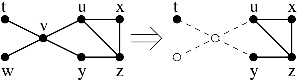
Leaf removal: If is a leaf of , and the subgraph of induced by , we say that is obtained from by leaf removal of . In other words, is obtained from by removing vertices and , the edge and all other edges touching . Note that this operation can destroy other leaves of and also create new leaves. See Fig. 1 for a pictorial example.
Step by step leaf removal process: Start from a graph . If has no leaves, stop. Else, choose a leaf and remove it, leading to a graph . If has no leaves, stop. Else, choose a leaf and remove it. This operation is iterated until no leaf remains.
History: A sequence associated to a step by step leaf removal process is called an history.
Isolated points, ; Core of a graph, : The last term in an history starting from is a graph which splits into a collection of isolated points , and an induced subgraph of without leaves or isolated points which we call the core of . We denote the number of points in the core by and the number of edges in the core by .
For these definitions to make sense, one has to show that the number of isolated points and the core are well defined, that is, do not depend on the choice of history. The formal proof is given in the appendix.
Global leaf removal process: Start from a graph . If it has no leaves, stop. Else select one leaf in every bunch of leaves. Remove from the vertex set both extremities of all the selected leaves, and define to be the set of remaining vertices. Let be the subgraph of induced by . Note that the leaves of (if any) are not leaves of . In this operation, the vertices belonging to a bunch of that were not selected become isolated points of . They remain isolated for the rest of the process. Iterate the procedure and define until a graph without leaves is obtained.
In the proof given in the appendix that the core is well-defined, the argument in step implies in particular that leaf removals that take place in distinct bunches of a graph commute. It implies that the global leaf removal process leads to same core and number of isolated points as any step by step leaf removal process.
While the global leaf removal process is convenient for analytical computations, the step by step leaf removal process is easier to implement on the computer.
4 Core percolation: infinite results
The global leaf removal process allows to compute the most salient characteristics of the leaf removal process, the functions , and . Remember that by definition, the number of isolated points after leaf removal is , the number of vertices in the core is , and the number of edges in the core is . The clue is an enumeration of all the configurations on the random graph that contribute extensively to the fundamental events in the global leaf removal process at step (which goes from to ): emergence of a new isolated point, removal of a point, removal of an edge111 The method of Refs. [3, 4] relies on approximate differential equations that apply to a slightly different model of random graphs. It is very powerful, but less intuitive than the direct enumeration method that follows. . This enumeration is possible because the finite configurations of vertices and edges in the random graph with extensive multiplicity are tree-like. This implies that the problem has a recursive structure. The weight of a tree is chosen so as to reproduce the correct random graph weight: a vertex has weight and an edge has weight . One has to be rather careful to avoid double counting and omissions; the examination of all cases is very tedious so we omit the details and simply outline the strategy.
The key ingredient is a study of leaf removal on rooted trees. Starting from a rooted tree, we apply the global leaf removal process, with the convention that even if the root has only one neighbor, it is not counted as a standard leaf222 However, a configuration where a neighbor of the root is a standard leaf is treated as usual. . We let be the generating function for rooted trees whose root becomes isolated exactly at step of the global leaf removal process, and be the generating function for rooted trees whose root is removed exactly at step of the global leaf removal process. For instance, counts rooted trees with an isolated root, hence trees with a single vertex, and . As another example, counts rooted trees whose root touches at least one standard leaf. Consider the trees whose root touches exactly standard leaves, and other vertices. These vertices can be seen as roots of non-trivial subtrees of the original tree, so by definition they contribute to . So the weight is
Hence
In the same way, contributions to or for larger s can be analyzed in terms of the trees attached to the neighbors of the root, and the structure of these trees involves lower order contributions. In contributions to , the root has at least one neighbor whose attached tree contributes to and any number of neighbors contributing to or or or . So
Analogously, in contributions to , the root has at least one neighbor whose attached tree contributes to and any number of neighbors none of which contributing to or or or . So
These two relations allow it to be shown that
where is the sequence of iterated exponentials, defined by
| (1) |
The events on the random graph that at step of the global leaf removal process a given vertex becomes isolated, or that a given vertex disappears, or that a given edge disappears can all be interpreted in terms of the previous configurations. In each case, the different possible contributions have to be taken into account, and also the rule that a root with a single neighbor can be touched by leaf removal has to be enforced. We omit this painful case by case analysis and only state the results.
The explicit formulæ for extensive contribution to the average number of isolated vertices, of non isolated vertices and of edges in are
| (2) | |||||
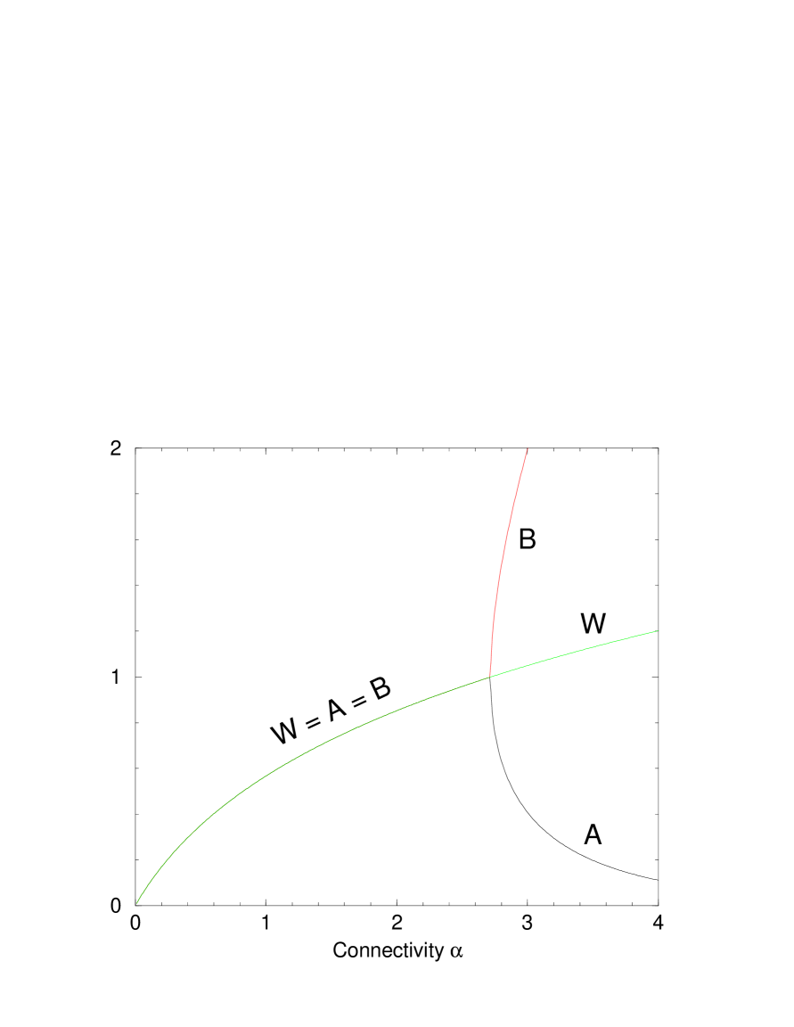
Now comes the crucial fact: when , the sequence converges to , where is the Lambert function, defined for as the unique real solution of the equation . The function is analytic for . When , remains a fixed point of the iteration Eq. (1) but it is unstable: the sequence is oscillating. However the even subsequence and odd subsequence are still convergent. The even limit is strictly larger than the odd limit. We define the functions and for by
Then solve the system
| (3) |
For , the unique solution is . For , the previous solution becomes unstable and is the solution of Eq. (3) selected by the rule . This is summarized on Fig. 2.
Taking the limit in Eq. (4) leads to
| (4) | |||||
For , , and the core indeed has a size . On the other hand, the core occupies a finite fraction of the vertices for . The behavior of Eq (1) is responsible for this geometric transition, core percolation, at . As and when , these functions are continuous but their derivatives are not: the transition is of second order. Note again that core percolation appears at , contrary to backbone percolation, which occurs at .
The fact that the core of a graph is an induced subgraph of the original graph allows to give a physicist’s argument for the uniqueness of the giant component in the core. Fix . If the core of the random graph contains two or more large connected components, there was no edge with extremities in two components in the original graph. But as the total size of the large connected components is of order , the absence of such an edge is extremely unlikely.
The behavior of thermodynamic functions close to the transition is the following. Writing , for small negative ,
while for small positive ,
For , this implies that there is a jump only in the second derivative of at the transition, with
while and have a jump in the first derivative at the transition, with
and
The expansion for contains only integral powers of , and this may be related to the fact (see section 5) that the finite size corrections for the number of edges in the core are slightly nicer than the ones for the number of vertices in the core . The average connectivity of the core is
for , which implies that giant core component should look like a large loop for close to . The exponent in the first correction makes such a property quite difficult to see numerically at large but finite .
In the random graph model, the vertices do not live in any ambient space, and the notion of correlation length is ambiguous. This problem will reappear in the finite size scaling analysis of the next section. However, the emergence of the core is very reminiscent of critical phenomena in physics. In particular, the critical slowing down is observable during the global leaf removal process. Indeed, the speed of convergence of the iterated exponential sequence can be computed. One finds that for , the convergence is exponential: the convergence rate is given by the formula
and more precisely
where , and are positive functions (they coincide for and ). When , , and when , .
At , the convergence is algebraic, and
This leads to the asymptotics at :
The first correction for is more important that the one for . Moreover the logarithms at lead to suspect that the finite size analysis of the next section might also be complicated by logarithms.
5 Numerical studies of the core percolation
The analytical computations above have enabled us to locate a phase transition at . They give information concerning the critical region but do not exhaust all the critical exponents. So we made an extensive numerical analysis of the core using Monte-Carlo simulations. At the first step this can also be used to check the previous analytical results. But let us start with the numerical algorithm.
5.1 Monte-Carlo algorithm
Our Monte-Carlo simulations consist in generating lots of random graphs, removing leaves step by step, and studying the remaining cores and isolated points. More precisely, for a given set of parameters , we generated random graphs in the microcanonical ensemble, with vertices and edges ( is rounded to the nearest integer value). In the microcanonical ensemble the total number of edges is fixed (in contrast to the canonical ensemble in which fluctuates).
As we want to simulate graphs with up to and with an average connectivity of order , we must use an algorithm which requires computer memory and time of order , not . With the microcanonical ensemble, the program is simpler: a random graph is obtained by choosing at random distinct edges among all the possible edges. From a Monte-Carlo point of view, the microcanonical ensemble has another advantage: the measurements fluctuate less.
As the graph (or equivalently its adjacency matrix) is very sparse, it is stored in an array of integers, indexed by an array of integers; the set of vertices adjacent to the vertex is the array section where . Then the connectivity of is . This defines the array , with the rules and .
Note that each edge appears twice in : once for and once for . This requires twice more memory than a storage method exploiting the symmetry of the matrix (in which the edges appear only once), but the computational task is faster because the adjacent vertices of a given vertex are simply obtained from arrays and .
The leaf removal process is done leaf by leaf. Each time a leaf is removed, the adjacent vertices are examined: if new leaves appear, there are added to a list of potential leaves to be considered later. Each elementary leaf removal requires a computational time of order and not . So the computational time for the global leaf removal is proportional to the number of removed leaves, which is bounded by . Then the total computational time for one random graph (generation and leaf removing) is times a function of .
For each random graph, we have measured the number of isolated points , the size (number of vertices) of the core , the number of edges of the core and consequently the average connectivity of the core : there are estimators of , , and , as defined before. As usual in Monte-Carlo simulations, averages have been done over many random graphs, and their confidence intervals (or error bars) are estimated by the variance of the measurements.
For each value of , we have generated graphs of size , and , and graphs of size and . At the transition value , graphs have been generated for all the sizes. The whole computation takes a few days on a medium Sun workstation without special optimization.
5.2 Monte-Carlo results
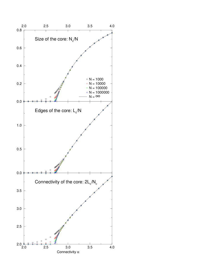
On Fig. 3, Monte-Carlo averages of , and are compared with the infinite results, , and . Errors bars are not drawn because they are smaller than the size of symbols. This figure is a typical case of a second order transition. Far from the transition, differences between finite and thermodynamic (i.e. ) functions are small. Finite size effects are at least of order , because the analytical calculations do not take into account the loops of finite size: their number is , so their contributions are . The simplest example is the “triangle” subgraph made of three vertices and three edges, not connected to the rest of the graph. Obviously, the triangles have no leaf and belong to the core: their contribution to is .
We have verified that finite size effects are of order (but not larger) for and far from the transition. For , this is probably true but less clear because fluctuations are stronger. On the other hand, in the critical region , finite size effects are larger and some critical exponents can be defined. They are discussed later.
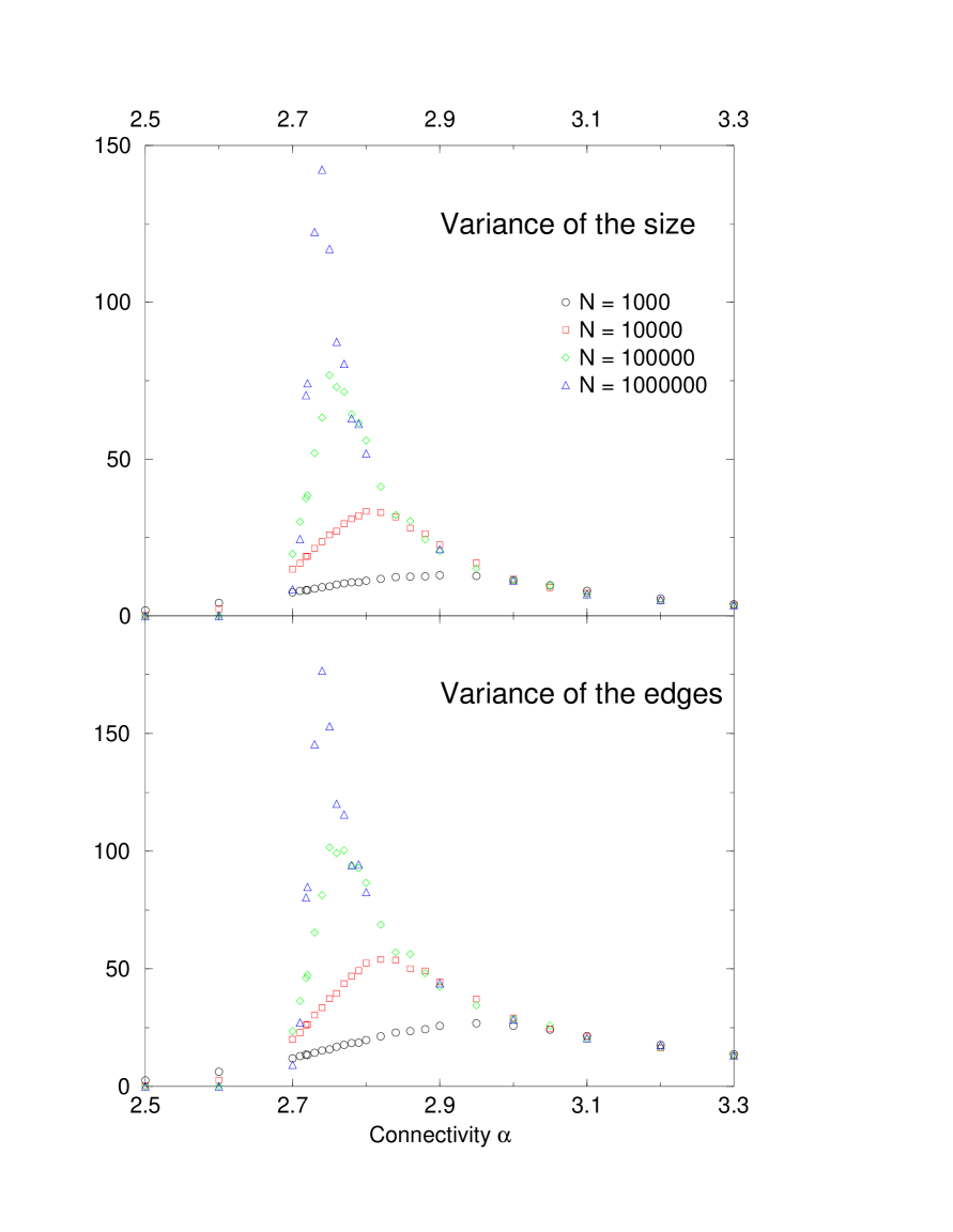
We have also examined the variances of the size, number of edges and average connectivity of the core. For not too close to and large , we expect that the fluctuations (square root of the variance) are of order for and , and for . So to obtain a large limit, we define , and . These quantities are analogous in the spin models to the magnetic susceptibility (equivalent to the fluctuations of the magnetization).
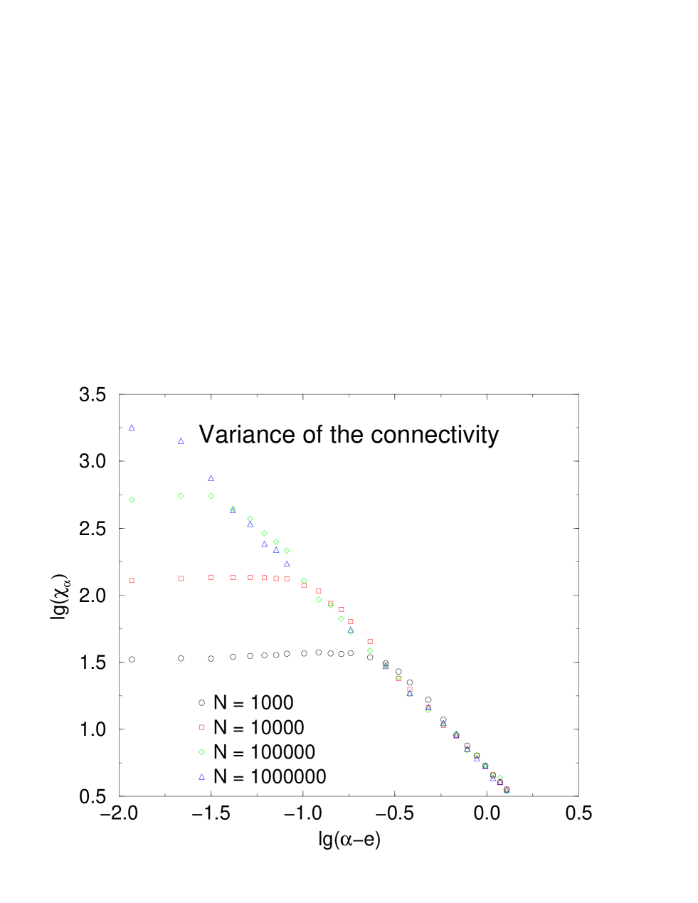
On Fig. 4, Monte-Carlo estimations of and show that and have a finite limit for when , a vanishing limit when and diverge when approaches the critical value . By analogy with and when , power laws are expected for the divergences. So, we define two critical exponents and by
| (5) | |||||
| (6) |
when . The exponent could be numerically measured by plotting or versus . Unfortunately, this gives poor results because the curvature of the plot is too important, with a slope changing from 1 to 0.5. But it is possible for . Fig. 5 is a log-log plot of versus . Symbols are lined up correctly and the global slope gives the estimation
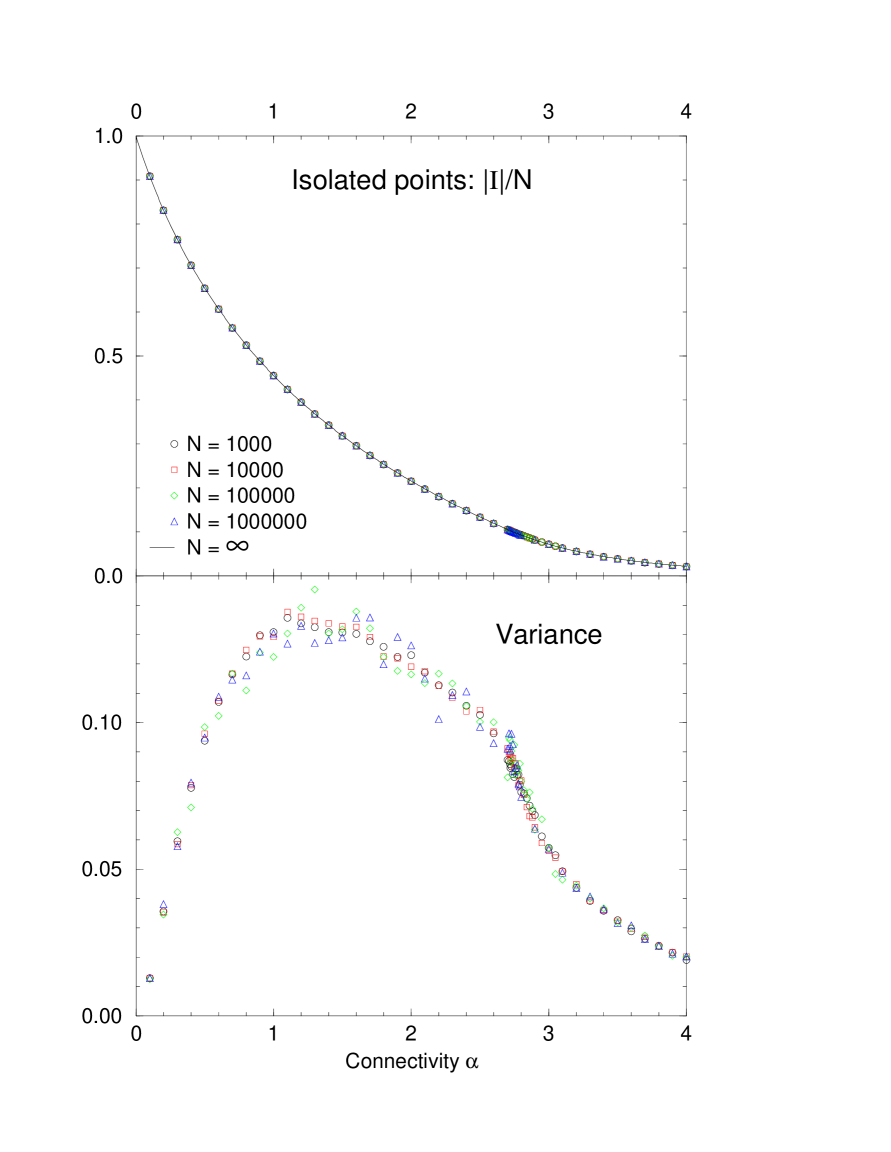
The studies of isolated points are resumed on Fig. 6. Monte-Carlo averages of are compared with the infinite results, : errors bars and finite size effects are so small that they are not visible. On the other hand, the variance shows bigger statistical fluctuations, but the finite size effects remain small. This variance does not diverge anywhere. However we see a cusp when compatible with
with estimations and . As , the first derivative is infinite at .
5.3 Finite size scaling
We now concentrate on the finite behavior, first exactly at the transition and then in the critical region around this transition.
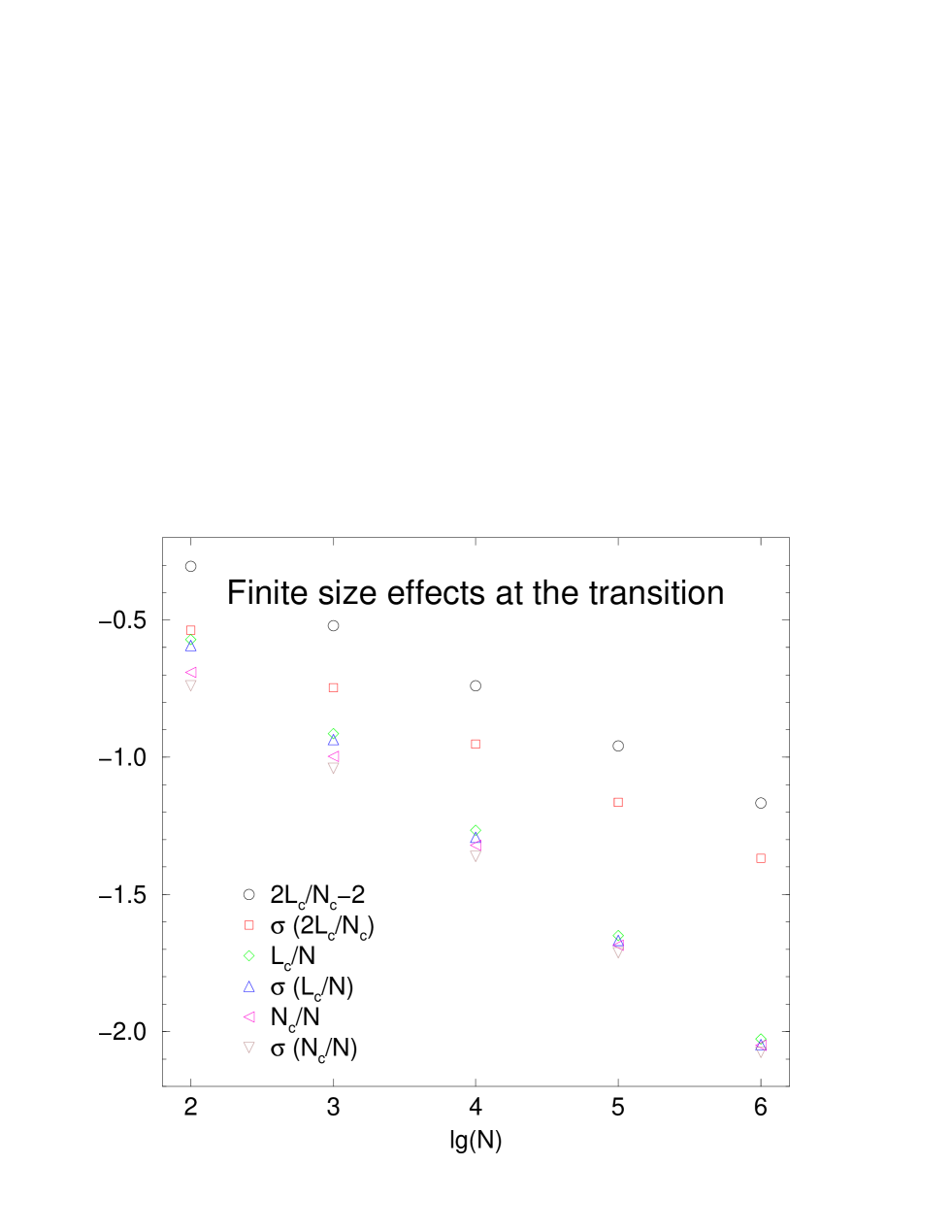
By analogy with the classical percolation transition at where the size of the largest connected component is [1] of order and its average connectivity is , we postulate the existence of other critical exponents and defined by
| (7) | |||||
| (8) |
when at . This hypothesis is tested on Fig. 7: data are correctly fitted by power-laws with
Of course, if the large behavior is modified by a (power of a) logarithmic function, the true values of the exponents are different than their apparent values when is large but finite. Here these exponents are determined by considering the averages of the Monte-Carlo measurements. The width of their distributions are also plotted on Fig. 7: means and widths have similar slopes. Consequently
| (9) |
diverge when at .
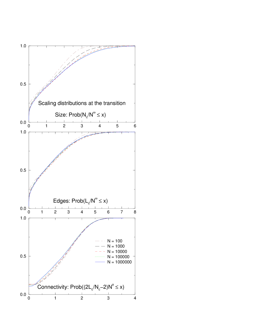
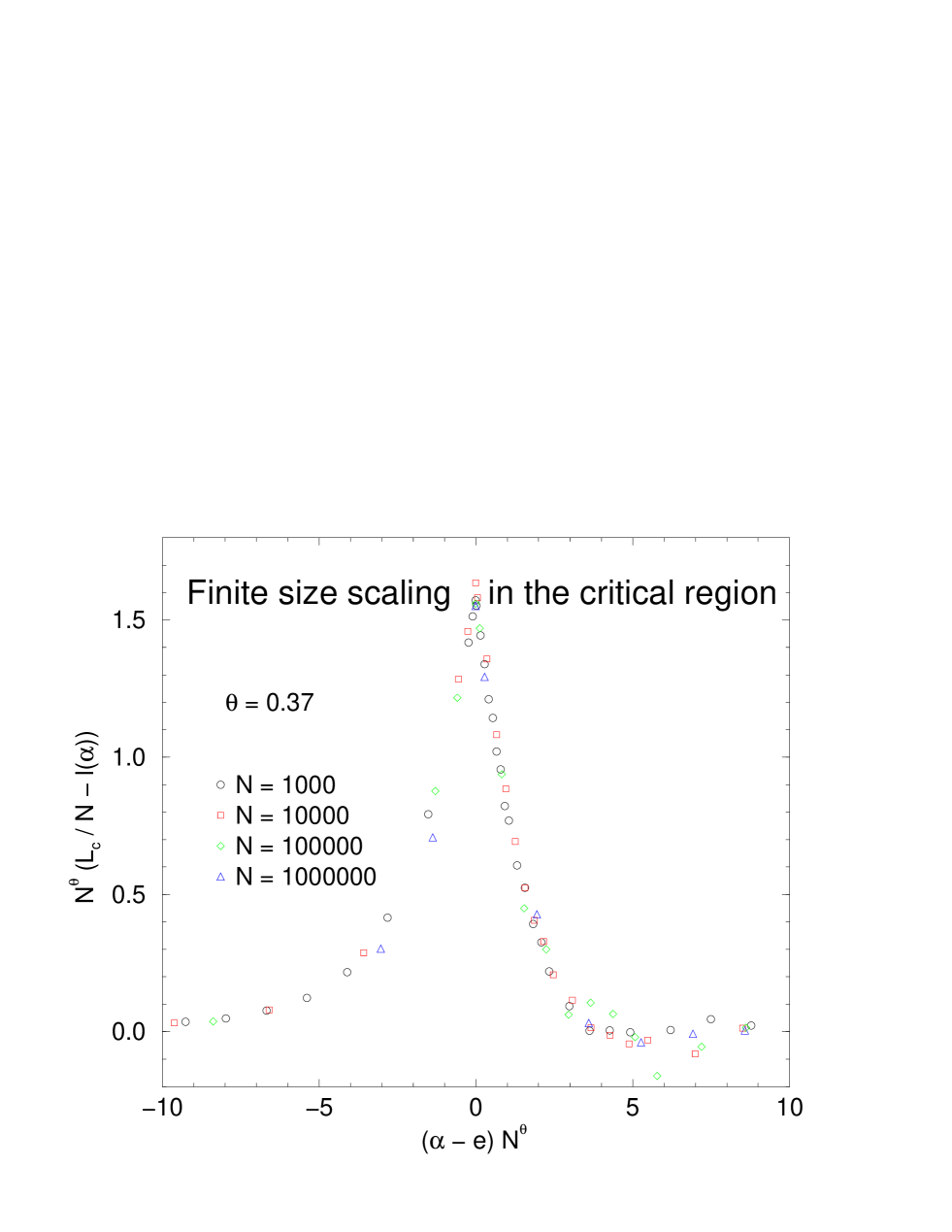
As widths and means of the Monte-Carlo measurements are of the same order, the distributions remain broad in the large limit at the transition. On the contrary, when , the distributions are sharp. On Fig. 8, the cumulative distribution functions Prob(, Prob( and Prob are plotted as functions of the scaling variable for . We observe that the curves converge when is large to scaling distributions (independent of ) and this confirms the hypotheses Eq. (7) and Eq. (8).
When becomes large, these scaling distribution functions decrease like a Gaussian. Consequently, they are not large distributions in the sense that every moment is finite, in agreement with Eq. (9). On the other side, these functions seem to be power laws for small . This allows to define another exponent with
| (10) |
when . Our estimation is
The numerical values suggest that , but we have no argument to explain it.
By considering the probability that the core of a random graph is void at , we measured a new exponent
where is defined by
The limit in Eq. (10) gives the conjectured relation , which is numerically acceptable. With the hypothesis , it gives .
We have also considered Prob, i.e. the probability that the average connectivity of the core is exactly 2. In this case, the core is made of one or several simple loops without branching. The Monte-Carlo study indicates that the large limit could be a pure number: 0.12(2). More intensive simulations are needed to confirm (or invalidate) this result.
More relations between critical exponents can be obtained by using the finite size scaling hypothesis [9]: in the vicinity of the transition, the behavior of finite random graphs is determined by the scaling variable
where is a positive scaling exponent.
First we shortly resume the scaling theory for a general quantity , for size and connectivity . For , let us suppose that
when ( could be positive or negative). Then we expect in the critical region that
where the scaling function is defined by
which behaves as
As exactly at the transition ,
So the exponent of finite size effects at the transition and the exponent of critical behavior for in the vicinity of the transition are related by . This remark is useful only if different quantities share the same . For usual models of statistical physics with a 2-D or 3-D geometry (like classical spin systems), the exponent describes the divergence of the correlation length . So the uniqueness of implies the uniqueness of . Unfortunately for random graphs, we have no equivalent length and no simple phenomenological interpretation for . However we shall assume that is unique.
As we have computed exact formulæ in Sect. 4, we can directly study , i.e. the finite size effects. The scaling function is now and is maximal around . From a numerical point of view, the analysis becomes easier than the one of the monotonic function .
Let us now consider and . As when , for these quantities . Then
On Fig. 9, with the choice (induced by the numerical measure of ), is plotted versus . We see that data are well superposed: they draw the scaling function. Note that is the unique fitting parameter for this figure.
Let us now consider the variances and . Using Eq. (5) and Eq. (9), the finite size scaling hypothesis gives the new relation
The same analysis with the average connectivity of the core can be done. As , the corresponding . Using Eq. (8), the scaling relation is
For the variance of the connectivity , Eq. (6) and Eq. (9) give
By eliminating , other relations are obtained: and .
| ’ | ||||||
|---|---|---|---|---|---|---|
| MC | 0.36(3) | 0.63(1) | 0.21(1) | 1.5(1) | 0.25(1) | |
| a | 1/3 | 2/3 | 1/6 | 1 | 2 | 2/9 |
| b | 0.37 | 0.63 | 0.185 | 0.70 | 1.70 | 0.233 |
| c | 2/5 | 3/5 | 1/5 | 1/2 | 3/2 | 24/100 |
| d | 0.42 | 0.58 | 0.21 | 0.38 | 1.38 | 0.244 |
With these four scaling relations and the Monte-Carlo determinations, we will now try to conjecture the exact values of these exponents. Table 1 resumes the following considerations. The results of Monte-Carlo simulations are given in line “MC”. Other lines are suggestions for sets of exponents compatible with the four scaling relations.
The line “b” is obtained by using the numerical determination of and the scaling relations. In particular, it gives . The line “d” uses the numerical determination of ; it gives . As the difference between these two values of is about twice larger than the uncertainty, we cannot definitely conclude whether the size and the connectivity of the core share the same scaling exponent or not.
The line “a” is obtained by assuming that and , which are the values [1] of the corresponding exponents for the classical percolation of random graphs at . This hypothesis seems incompatible with the Monte-Carlo estimations of and . Furthermore the average connectivity of the giant component near the classical percolation transition behaves with — to be compared with for the core — and consequently the corresponding exponent is (but not ).
This gives strong evidence that the analogy between exponents of percolation and core transitions cannot be complete and that the effective low energy field theory descriptions in the vicinity of the transition are different. In particular, they may well have a different upper critical dimension.
The line “c” assumes that the exponent is exactly . This is very attractive because exponents are simple rational fractions and the value is between the numerical estimations and .
Of course, nothing in the theory of critical phenomena requires that critical exponent are rational numbers with small numerators (for a recent example, see Ref [10]). However, if we want conciliate numerical simulations, theoretical considerations and simple rational fractions, we are led to conjecture , , , , and .
To reduce the uncertainties in Monte-Carlo simulations, bigger size are needed, in particular in the case where the large behavior would be affected by logarithmic laws. Moreover, we hope to progress in analytical methods for calculating these exponents as well.
6 Applications
We now discuss two applications of the structure of the core: the first one to the conductor-insulator transitions in random graphs and the second one to combinatorial optimization problems.
6.1 Localization on random graphs
We denote by the dimension of the kernel (the subspace of eigenvectors with eigenvalue ) of the adjacency matrix of the graph . It is known [11] that is invariant under leaf removal (see Ref. [12] for a proof and an application to random trees). As the adjacency matrix is block-diagonal with one block per connected component, is additive on connected components. These two properties imply that
The last equality is because the adjacency matrix vanishes for a collection of isolated points. This analysis applies to any graph, and remains valid after averaging. Even if the probability distribution is not that of a random graph, we see that as soon as leaves appear with a non vanishing weight (this is true for instance if the probability distribution is that of a lattice with impurities), the spectrum of the adjacency matrix has a delta peak at the origin. However, the fact that, as we show below for random graphs, leaf removal accounts for the full weight of this delta peak seems rather non generic.
Taking the average of these formulæ for random graphs and using our results on the core, we get that for a large random graph with average connectivity , with
| (11) | |||
It has been argued in Ref. [7] that
| (12) |
for all values of . Combined with our present results, this means that
We may interpret Eq. (11) as an independent proof of Eq. (12) for and we may also infer that the adjacency matrix of the core of a random graph at has a kernel of size .
In Ref. [7], it was shown that is in a domain of the parameter for which delocalized vectors are responsible for a finite fraction of the size of the kernel. Imagine that we start to increase very slowly from by adding randomly new edges one by one to the random graph. We watch the competition between the core (which, we have seen, carries few elements in the kernel), the localized eigenvectors in the kernel and the delocalized ones. The competition between the core and the full kernel is not very strong: when edges, with , are added to the graph, the core grows in average of vertices, while vectors in the kernel are lost. However, by the results of Ref. [7], about delocalized eigenvectors disappear and localized eigenvectors replace these. It is intuitive that delocalized eigenvectors in the kernel, which live on large structures on the random graph, have a high probability to be perturbed by the growing core. But the precise mechanism by which their extinction is almost compensated by new localized vectors in the kernel remains to be elucidated.
The concept of leaf removal process can also be used to analyze the localization-delocalization transitions that occur at and . As shown in Ref. [7], the localized eigenvectors in the kernel live on definite structures that can be drawn on the random graph. These structures are finite (connected) trees that
-
•
can be bicolored brown-green in such a way that all vertices with 0 or 1 neighbor are green and all neighbors of the green vertices in the random graph belong to the tree; the neighbors of the brown vertices on the other hand, can be anywhere on the random graph.
-
•
are maximal, i.e. are not part of a larger tree with the same properties. Observe that each isolated point is maximal.
We can put marks on all vertices belonging to such structures and build histories of leaf removal processes such that the initial steps remove only marked vertices, and after these steps, the only remaining marked vertices are now isolated.
Then if is small () or large (), the number of isolated marked points is . This implies in particular that at most bunches of the remaining graph contain more than one leaf.
On the other hand, if the number of isolated marked points is less than : a number of order of non-trivial bunches will have to appear somewhere during the rest of the leaf removal process.
6.2 Vertex covers and matchings
Apart from the size of the kernel, several other interesting quantities attached to graphs behave rather simply under leaf removal. We mention two, which are related to combinatorial optimization problems.
Vertex cover: A vertex cover of a graph is a subset of the vertices containing at least one extremity of every edge of the graph. We denote by the minimal size of a vertex cover of a graph .
There is a nice “practical” interpretation of . Imagine that the edges of the graph are the (linear) corridors of a museum, the vertices corresponding to ends of corridors. A guard sitting at a vertex can control all the incident corridors. So is the minimum number of guards needed to control all corridors of the museum.
Edge disjoint subset, matching: An edge disjoint subset is a subset of the edges such that no two edges in the subset have a vertex in common. This is also called a matching. We denote by the maximal size of edge disjoint subset in a graph . Finding such a maximal edge disjoint subset is called the matching problem.
The determination of or for a given are archetypal of two classes of optimization problems. While it is known that the matching problem can be solved in polynomial time (see e.g. Ref.[4] and references therein), the museum guard problem is in the Non-deterministic Polynomial (NP) class because no polynomial time algorithm is known to solve it (and such an algorithm is not expected to exist, this is related to the famous PNP conjecture), but given a candidate solution, it is easy to check in polynomial time that it is correct.
When is a large random graph, one may ask for thermodynamic solutions of these problems, when only the extensive contributions to or are considered as relevant. This leads to the following definition:
Vertex cover fraction , matching fraction : For fixed , the vertex cover fraction and the matching fraction are the limits of the averages of and when is a random graph of size and .
Let us note however that the one can probably exhibit combinatorial optimization problems for which the thermodynamic solution can be obtained in polynomial time, but taking into account the non-extensive remainder is prohibitively long.
The replica trick has been used by Hartmann and Weigt to obtain a lower bound for in a series of papers [6, 13, 14]. They have shown that for , the replica symmetric solution is stable, whereas it become unstable for . The replica symmetric solution leads to
This relation has to break down somewhere, because a result of Frieze [15] implies that
whereas for large , so that the asymptotics of starts with . Weigt and Hartmann [14] have also used a good algorithm to get an approximation of a minimal vertex cover. The idea is essentially to look for a vertex with a maximal number of incident corridors and put a guard there. Then remove the site and the adjacent corridors and iterate. This is always fast, but gives only an upper bound for . This can be refined, but then the algorithm needs a very long time when .
We show how leaf removal can be applied to the museum guard problem. If is a leaf of , there is a minimal vertex cover with a guard at . This is because any vertex cover has a guard at or at , and a guard at makes the guard at useless. So if a minimal vertex cover has a guard at , moving it to yields another minimal vertex cover. Isolated vertices do not need guards. The leaf removal of leading from to removes exactly the corridors controlled by the guard at . Hence .
An analogous argument applies to maximum edge disjoint subsets. Indeed, if is a leaf of , there is a maximal edge disjoint subset that contains . This is because if no edge of an edge disjoint subset touches , this edge disjoint subset is not maximal (it can be completed with ), and if an edge disjoint subset has an edge that touches , replacing this edge by yields an edge disjoint subset of the same size. The leaf removal of leading from to removes, apart from , exactly the edges that cannot belong to any edge disjoint subset containing . Hence .
Some general inequalities can be proved. For instance (the triangle is an example when the inequality is strict) and . However, can have any sign (negative for the triangle but positive for the square).
Anyway, at each leaf removal, two vertices are removed, so , and are invariant under leaf removal. Moreover, and vanish for unions of isolated vertices. To summarize,
Karp and Sipser [3, 4] have devised an approximate algorithm to get a good (if not optimal) matching. There are two possible transformations:
(1) Remove a leaf,
(2) Choose an edge at random, remove it together with its extremities and all edges touching the extremities.
and they are are performed according to the following rule:
At each step, until the graph is empty, do (1) if possible and if not, do (2). So starting from , one applies (1) until the core of is obtained. Then (2) is applied as long as no new leaf appears. As soon as a graph with leaves appears, apply (1) to reach the core of this new graph, and so on.
At each step an edge is singled out, and by construction, the set of all these edges defines a matching, i.e. an edge disjoint subset.
When is a random graph with , the core is small ( for large ). Thus,
which gives in particular an independent proof of the result of Weigt and Hartmann [6]. Note that in this case, the approximate algorithm is to put a guard at a vertex touching as many edges as possible, then remove it and iterate, whereas the exact algorithm is almost the opposite, namely, put a guard at the connected end of a leaf, remove the leaf and iterate. Leaf removal gives a very fast algorithm (linear in if the graph is properly encoded) to construct a minimal vertex cover when .
Karp and Sipser have shown that for a large random graph with , their algorithm for matching finds with high probability a matching of about edges in the core. This is a lower bound for the matching number of the core, but at the same time, this is the maximum possible. So this shows at once that the core has a thermodynamically perfect matching, and that their algorithm is thermodynamically optimal. Hence
so that the relation is valid for every : the fact that the core does not contribute thermodynamically to zero eigenvalues and the fact that it has a thermodynamically perfect matching are closely related.
If , leaf removal stops while an extensive number of edges are still present: this gives a lower bound for which is very poor at large . But it seems clear that the replica symmetry breaking [14] at is tightly connected to the fact that the structure of the core of a random graph is more complicated than the structure of the parts eliminated by leaf removal, so that a more refined Parisi order parameter is needed to describe the phase . While we have seen that the matching parameter and the kernel-size parameter are well understood and closely related, the exact evaluation of vertex cover parameter remains as a challenge.
7 Conclusions
In this paper we have presented a physicist’s analysis of a deep feature of random graphs : a geometric second order phase transition with the emergence of a core at threshold . This core is the residue when leaves (i.e. points with a single neighbor and this neighbor) and isolated points are iteratively removed. We have argued that the core is dominated by a giant component. The dominant contribution of the large behavior of the relevant thermodynamic quantities was computed exactly by a direct counting method. We have studied numerically the finite size behavior of the core, defined a variety of new critical exponents and obtained approximations consistent with their mutual relationships. Our analysis excludes the exponents of standard percolation in random graphs. Finally, we have applied our results to the localization transition and to combinatorial optimization problems on random graphs.
However, some more analytical or numerical work is needed to identify without any doubt the exponents for the phase transition at . An open question is the interaction between the emergence of the core and the delocalized eigenvectors of the adjacent matrix with eigenvalue 0. A fine study of the distribution of the sizes of the connected components of the core could be done with Monte-Carlo simulations: for , we expect a giant component, plus a finite number of finite components. Moreover we have shown that the number of eigenvectors with eigenvalue 0 living on the core is and numerical simulations could give the precise asymptotics.
Finally, as the core percolation appears in a simple model of random graphs, which is governed only by one parameter, the average connectivity , we expect that this transition is universal in the sense that some characteristics of this transition (second order, critical exponents, etc., but not the precise value of at the transition) could be seen in other models or real materials.
Acknowledgments: We are very indebted to Graham Brightwell and Boris Pittel for drawing our attention to the mathematical literature on matching in random graphs and its relevance for our work.
Appendix A ppendix: The core is well-defined
In this appendix, we show by induction on the number of vertices of that the property
“the number of isolated points after leaf removal and the core of a graph on vertices do not depend on the history”
holds for any .
To start the induction, if has 0 or 1 vertex, there is no leaf hence there is only one history, so and are true. Suppose now that are proved and take a graph on vertices. We distinguish several cases:
- 1
-
If has no leaf, there is only one history so is true for .
- 2
-
If has exactly one leaf, all histories start with the same first leaf removal, lead to the same for which is true by the induction hypothesis, so is true for .
- 3
-
If has at least two leaves, we compare two histories:
- 3a
-
If , to which the induction hypothesis applies, so that and .
- 3b
-
If but (the two leaves are distinct but belong to the same bunch, this can happen only if ), then has as an isolated point, has as an isolated point, but , say. Further leaf removals can take place only on , to which the induction hypothesis applies, so again, and .
- 3c
-
Suppose that and do not belong to the same bunch. This can happen only if . Then is a leaf of and is a leaf of . The graph obtained from by leaf removal of and the graph obtained from by leaf removal of are the same, because they are both equal to , the subgraph of induced by . Take a history for . It can be completed to give two histories for G, and . The induction hypothesis applies to so and have to end with the same core and the same number of isolated points. The same is true for and because the induction hypothesis applies to , and also for and because the induction hypothesis applies to . By transitivity, and end with the same core and the same number of isolated points: and .
All possibilities have been examined, hence whatever the number of leaves of , is true for . This completes the induction step.
References
- [1] P. Erdös and A. Rényi, On the evolution of random graphs, Publ. Math. Inst. Hungar. Acad. Sci. 5 (1960), 17–61.
- [2] S. Janson, D.E. Knuth, T. Luczak and B. Pittel, The birth of the giant component, Random Structures and Algorithms 4 (1993), 233–358.
- [3] R.M. Karp and M. Sipser, Maximum matchings in sparse random graphs, Proceedings of the 22nd IEEE Symposium on Foundations of Computing (1981), 364–375.
- [4] J. Aronson, A. Frieze and B.G. Pittel, Maximum matchings in sparse random graphs, Karp-Sipser revisited, Random Structures and Algorithms 12 (1998), 111–177.
- [5] B. Bollobás and G. Brightwell, The width of random graph orders, Math. Scientist 20 (1995), 69–90.
- [6] M. Weigt and A.K. Hartmann, Number of guards needed by a museum: a phase transition in vertex covering of random graphs, Phys. Rev. Lett. 84 (2000), 6118–6121, arXiv:cond-mat/0001137.
- [7] M. Bauer and O. Golinelli, Exactly solvable model with two conductor-insulator transitions driven by impurities, Phys. Rev. Lett. 86 (2001), 2621–2624, arXiv:cond-mat/0006472.
- [8] M. Bauer and O. Golinelli, Random incidence matrices: moments of the spectral density, J. Stat. Phys 103 (2001), 301–337, arXiv:cond-mat/0007127.
- [9] For a general presentation, see M. N. Barber, Finite-size scaling, in Vol. 8 of Phase transitions and critical phenomena, edited by C.Domb and J. L. Lebowitz (Academic Press 1983).
- [10] P. Di Francesco, O. Golinelli, E. Guitter, Meanders: exact asymptotics, Nucl. Phys. B 570 (2000), 699–712, arXiv:cond-mat/9910453.
- [11] D.-M. Cvetković, M. Doob and H. Sachs, Spectra of Graphs, Academic Press, New York, 1980.
-
[12]
M. Bauer and O. Golinelli,
On the kernel of tree incidence matrices,
J. Integer Sequences, Article 00.1.4, Vol. 3 (2000),
http://www.research.att.com/njas/sequences/JIS. - [13] A.K. Hartmann and M. Weigt, Statistical mechanics perspective on the phase transition in vertex covering of finite connectivity random graphs, Theoretical Computer Science 265 (2001), 199, arXiv:cond-mat/0006316.
- [14] M. Weigt and A.K. Hartmann, Minimal vertex covers on finite-connectivity random graphs — a hard-sphere lattice-gas picture, Phys. Rev. E 63 (2001), 56–127, arXiv:cond-mat/0011446.
- [15] A.M. Frieze, On the independence number of random graphs, Discr. Math. 81 (1990), 171.