Bose condensation of cavity polaritons beyond the linear regime: the thermal equilibrium of a model microcavity.

Abstract

We consider a generalization of the Dicke model. It describes localized, physically separated, saturable excitations, such as excitons bound on impurities, coupled to a single long-lived mode of an optical cavity. We consider the thermal equilibrium of the model at a fixed total number of excitons and photons. We find a phase in which both the cavity field and the excitonic polarization are coherent. This phase corresponds to a Bose condensate of cavity polaritons, generalized to allow for the fermionic internal structure of the excitons. It is separated from the normal state by an unusual reentrant phase boundary. We calculate the excitation energies of the model, and hence the optical absorption spectra of the cavity. In the condensed phase the absorption spectrum is gapped. The presence of a gap distinguishes the polariton condensate from the normal state and from a conventional laser, even when the inhomogeneous linewidth of the excitons is so large that there is no observable polariton splitting in the normal state.

I Introduction

In the strong-coupling regime for matter and light, radiative decay of a material excitation gives way to coupled oscillations of the polarization of the matter and of the electromagnetic field. The quasiparticles corresponding to such coupled modes are known as polaritons [1]. The classic realization of polaritons is excitons in a bulk semiconductor coupled to photons in free space, as discussed many years ago by Hopfield [2]. In this example, wavevector conservation ensures that each exciton is coupled only to a single mode of the electromagnetic field, leading to the formation of polaritons which are superpositions of a single exciton and photon. Recently, there has been a lot of interest in polaritons formed from photons confined in cavities: such cavity polaritons have now been observed for confined photons coupled to atoms [3], to two-dimensional excitons in quantum wells [4], to bulk excitons [5], to excitons in films of organic semiconductors [6, 7], and to charged exciton complexes [8].

Since polaritons are photons coupled to other excitations, they are bosons, and so are candidates for Bose condensation [9]. Recent observations [10, 11, 12, 13, 14] of bosonic behavior for cavity polaritons have renewed interest in this idea.

However, there is a conceptual difficulty with a Bose condensate of polaritons: while polaritons are usually considered in the low-excitation linear regime, Bose condensates are stabilized by nonlinearities [15]. For cavity polaritons, there is also the following more practical difficulty. Bose condensates are characterized by coherence, and in a polariton condensate this coherence will appear in the photons. Given this, how is a polariton condensate distinct, conceptually and observationally, from a laser?

In this paper we address these problems by developing a theory of polariton condensation in the Dicke model [16]. This nonlinear model of confined photons coupled to matter is one of the basic models of laser physics. It allows us to go beyond the conventional linear-response concept of a polariton, including effects due to finite excitations of the matter in the cavity. In the language of semiconductors, it includes a “saturation” or “band-filling” nonlinearity, produced by the fermionic internal structure of the excitons.

Polaritons are not conserved particles, so there is ultimately no equilibrium condensate. We may, however, treat polaritons as conserved particles if their lifetime is much longer than the time required to achieve thermal equilibrium at a fixed polariton number. We will study this quasi-equilibrium regime, since it is in this regime that Bose condensation is well-defined [9].

In section II, we introduce the model, and explain how the concept of a polariton can be generalized to allow for the nonlinearity of the model. We then present, in sections III and IV, a simple variational technique for calculating the ground state of the model at a fixed density of polaritons. In section V we investigate the thermodynamics of the model using an alternative technique based on functional integrals. This technique demonstrates that the variational approach is essentially exact, and allows us to consider finite temperatures. In section VI, we use the expressions derived by the functional integral method to study the phase diagram for condensation, while in section VII, we use these expressions to calculate the excitation spectra of the model. These excitation spectra provide a physical picture of the transition to the condensed state, and determine the absorption spectrum of the cavity. Finally, in section VIII we discuss our conclusions.

The functional integral approach to the thermodynamics of our model has already been the subject of a brief report [17]. We extend that earlier report to allow for a distribution of the energies of the electronic excitations, i.e. inhomogeneous broadening, which is significant in many potential realizations of the polariton condensate.

II Model

The Dicke model [16, 18] consists of a set of $N$ two-level oscillators coupled to a single mode of the electromagnetic field by the dipole interaction. The two-level oscillators do not interact with one another, except through their common coupling to the electromagnetic field. We generalize the original Dicke model to include an energy distribution of the two-level oscillators. Making the rotating-wave approximation(see e.g. Refs. [18, 19]), we consider the Hamiltonian

$$H=\sum\frac{E_{g}(n)}{2}\left(b^{\dagger}b-a^{\dagger}a\right)+\omega_{c}\psi^{\dagger}\psi+H^{\prime},$$ (1)

$$H^{\prime}=\frac{g}{\sqrt{N}}\sum\left(b^{\dagger}a\psi+\psi^{\dagger}a^{\dagger}b\right).$$ (2)

Here the two-level oscillators are indexed by the variable $n$, which is summed over. We use a fermionic representation for the two-level oscillators, describing each one in terms of a pair of fermions with annihilation operators $a$ and $b$. For brevity we suppress the index $n$ on the fermionic operators. The fermions are subject to the single-occupancy constraint

$$b^{\dagger}b+a^{\dagger}a=1$$ (3)

on each site. $\psi$ is the annihilation operator for the cavity mode, $E_{g}(n)$ is the energy of the $n^{th}$ two-level oscillator, and $g$ is the strength of the dipole coupling.

The Hamiltonian (1) is a simple model of a three-dimensional cavity (photonic dot) [20, 21], containing localized, physically separated electronic excitations. Although simplified, it is a useful starting point for many systems. For example, each of the two-level oscillators could describe the presence or absence of a localized exciton in a given eigenstate of the disorder potential in a disordered quantum well, on a given molecule in an organic film, or trapped on a particular impurity. The restriction to singly occupied states models the hard-core repulsion produced by the fermionic structure of such excitations. It describes spinless excitations which are localized on the scale of the (exciton) Bohr radius. It is straightforward to generalize our calculations to allow for a finite number of excitations on each site, i.e. traps which are bigger than the Bohr radius, and so can hold several excitons.

$H^{\prime}$ couples the photons to excitations of the two-level oscillators, created by the operator $S_{+}=\frac{1}{\sqrt{N}}\sum b^{\dagger}a$. If $E_{g}(n)=E_{g}$ then the excited states which are created by $S_{+}$ from the vacuum are eigenstates of the bare Hamiltonian $H$. If furthermore $N$ is large and the two-level oscillators are near to their ground state,

$$\frac{1}{2}\sum\langle b^{\dagger}b-a^{\dagger}a\rangle\approx-N/2,$$ (4)

then $S_{+}$ is approximately a bosonic creation operator, and the Hamiltonian (1) becomes two coupled boson oscillators. Polaritons are usually presented as the eigenstates of such a model.

Away from the low-excitation limit (4), $S_{+}$ is not a bosonic creation operator, and the conventional description of polaritons breaks down. To go beyond the low-excitation limit, we generalize the concept of a polariton to be the quantum of excitation of the coupled matter-light system. The polariton number is then the total number of photons and excited two-level oscillators,

$$N_{\mathrm{pol}} = L+N/2$$ (5)

$$= \psi^{\dagger}\psi+\frac{1}{2}\sum b^{\dagger}b-a^{\dagger}a+N/2,$$ (6)

which is a conserved quantity for the model (1). (5) defines the operator $L$, which we refer to as the excitation number. We define a corresponding excitation density $\rho_{ex}=\langle L\rangle/N$, which is the total number of photons and electronic excitations, per two-level oscillator, minus one-half. Since the numbers of photons and electronic excitations are positive, the lowest excitation density is $-0.5$. Since the number of electronic excitations is always less than $N$, the electronic contribution to $\rho_{ex}$ is always less than $0.5$.

The thermal equilibrium of the Dicke model, in the absence of an externally created population of polaritons, has been studied extensively since the pioneering exact solution of Hepp and Lieb [23]. These authors showed that, even in the absence of external excitation, the Dicke model has a phase transition to a Bose condensed state. Such an equilibrium condensate is a static, coherent state of photons: it is a ferroelectric [24]. Here we are interested in the thermal equilibrium of a population of polaritons: the quasi-equilibrium problem posed by (1) at a fixed excitation $L$. The quasi-equilibrium condensate which we find in this regime is a time-varying generalization of the ferroelectric state discovered by Hepp and Lieb.

III Variational approach

We can write down a variational state which describes the polariton condensate by noting that Bose condensates are described by coherent states. This produces a variational wavefunction closely related to the BCS wavefunction used to describe superconductors and exciton condensates. As has been stressed by Comte and Nozières [25], this class of wavefunction can describe an exciton condensate in both the low and high density limits. It thus permits a smooth interpolation from low densities, where the excitons are simple bosons, to high densities, where their fermionic internal structure is revealed. In a similar way, it allows us to explore the polariton condensate beyond the low-density regime in which polaritons are usually considered.

The constituents of our proposed condensate are the excitations of the whole system, counted by $L$. In general, such an excitation is a superposition of an excitation of the cavity mode and an excitation of the electronic states. Thus we take for our trial wave-function a coherent state of such a superposition:

$$|\lambda,w\rangle=e^{\lambda\psi^{\dagger}+\frac{1}{\sqrt{N}}\sum_{n}w_{n}b^{\dagger}a}|vac\rangle,$$ (7)

where the state $|vac\rangle$ has a single fermion in the lower state of each two-level oscillator. The state (7) has a finite polarization of the electronic excitations as well as a finite amplitude for the cavity field. $\lambda$ and $w_{n}$ are the variational parameters. Expanding the exponential, (7) explicitly becomes a superposition of a coherent state of photons and a BCS state of the fermions,

$$|\lambda,u,v\rangle=e^{\lambda\psi^{\dagger}}\prod_{n}(v_{n}b^{\dagger}+u_{n}e^{i\phi_{n}}a^{\dagger})|0\rangle.$$ (8)

Here $\lambda,u_{n},v_{n}$, and $\phi_{n}$ are the variational parameters, and $|0\rangle$ denotes the vacuum state with no fermions in any of the levels. By construction, this variational state obeys the single-occupancy constraints (3). We fix the overall phase of the condensate by choosing $\lambda$ to be real. The $\phi_{n}$ have been explicitly introduced to make the $u$ and $v$ real. They are the phase differences between the cavity field and the polarizations of the electronic states.

To find the ground state of (1) at fixed excitation number we minimize

$$\langle H-\mu_{ex}L\rangle = \tilde{\omega}_{c}\lambda^{2}+\sum_{n}\tilde{\varepsilon}_{n}(v_{n}^{2}-u_{n}^{2})$$ (10)

$$+2\frac{g}{\sqrt{N}}\lambda u_{n}v_{n}\cos(\phi_{n}),$$

$$\tilde{\omega}_{c} = \omega_{c}-\mu_{ex},$$ (11)

$$\tilde{\varepsilon}_{n} = \frac{E_{g}(n)-\mu_{ex}}{2},$$ (12)

with respect to the variational parameters, subject to the normalization conditions $u^{2}_{n}+v^{2}_{n}=1$.

Although the overall phase of the condensate is arbitrary, the relative phases $\phi_{n}$ are not: there is only one order parameter. The relative phases $\phi_{n}$ are fixed by the last term in (10), the dipole coupling. This term ensures that all the two-level oscillators which have a finite dipole moment($u_{n}\neq 0,1$) are mutually coherent, $\phi_{n}=\phi$, when the energy is minimized. It is the dipole interaction which is responsible for Bose condensation, and its accompanying coherence [15], in the present system.

Setting $\phi_{n}=0$ and defining an intensive $\lambda$ by rescaling $\lambda\to\lambda\sqrt{N}$, the condensate parameters are given by the real solutions with $\lambda u_{n}v_{n}<0$ to

$$\tilde{\omega}_{c}\lambda+\frac{g}{N}\sum_{n}u_{n}v_{n}=0,$$ (13)

$$2\tilde{\varepsilon}_{n}u_{n}v_{n}-g\lambda(v_{n}^{2}-u_{n}^{2})=0.$$ (14)

$\mu_{ex}$ was introduced as a Lagrange multiplier constraining the excitation number. It is the chemical potential for our coupled modes, and is related implicitly to the excitation density by

$$\rho_{ex} = \frac{1}{N}\left\langle\psi^{\dagger}\psi+\frac{1}{2}\sum b^{\dagger}b-a^{\dagger}a\right\rangle$$ (15)

$$= \lambda^{2}+\frac{1}{2N}\sum_{n}v^{2}_{n}-u^{2}_{n}.$$ (16)

Eliminating $u_{n}$ and $v_{n}$ from (13) and (15) we can rewrite these expressions as

$$\tilde{\omega}_{c}\lambda=\frac{g^{2}\lambda}{2N}\sum_{n}\frac{1}{|E_{n}|},$$ (17)

$$\rho_{ex}=\lambda^{2}-\frac{1}{2N}\sum_{n}\frac{\tilde{\varepsilon}_{n}}{|E_{n}|},$$ (18)

where we define

$$E_{n}=\mathrm{sign}(\tilde{\varepsilon}_{n})\sqrt{\tilde{\varepsilon}^{2}_{n}+g^{2}|\lambda|^{2}}.$$ (19)

(17) is analogous to the BCS gap equation, with an order parameter $\lambda$.

IV Zero temperature properties

To investigate the expressions (17–19), we replace the summations over sites with an integral over the energy distribution of the two-level oscillators. We take this distribution to be a Gaussian with mean $E_{0}$ and variance $\sigma g$. The remaining parameters in our quasi-equilibrium problem are then the excitation density, $\rho_{ex}$, and the dimensionless detuning between the energy of the cavity mode and the center of the exciton line, $\Delta=(\omega_{c}-E_{0})/g$.

For a Gaussian density of states, the summation on the right of (17) diverges as $\lambda\to 0$, and approaches zero as $\lambda\to\infty$. Thus for any $\mu_{ex}<\omega_{c}$ there is always a condensed solution, $\lambda\neq 0$, to (17): the system is condensed at arbitrarily small excitation densities. This behavior is produced by the tails of the Gaussian distribution. Because of these tails, we have excitons at arbitrarily low energies, and hence also bound exciton-photon states at arbitrarily low energies. It is impossible to populate just the excitons, because no matter how small $\mu_{ex}$ is, there is always a bound state involving photons below it. We expect that if the density of states has a lower cut-off, and is continuous at this cut-off, there would be a finite critical $\mu_{ex}$ below which there is no condensed solution to (17).

Let us investigate the dependence of $\mu_{ex}$ on $\rho_{ex}$ in the absence of inhomogeneous broadening, $\sigma=0$. At low densities, $\rho_{ex}\approx-0.5$, $\mu_{ex}$ can be obtained from (17). Expanding this expression for small $\lambda$ and comparing the leading terms, we find that $\mu_{ex}$ is given by the conventional linear-response polariton energy, $\mu_{ex}=E_{\mathrm{LPB}}=\frac{1}{2}[(\omega_{c}+E_{g})-g\sqrt{\Delta^{2}+4}]$. At finite densities we calculate $\mu_{ex}$ numerically, by solving (17) and (18) to determine $\rho_{ex}(\mu_{ex})$. The results are plotted in the right panel of Fig. 1, for $\Delta=0,1$ and $3$. At low densities we are describing a condensate of conventional polaritons, and so have $\mu_{ex}=E_{\mathrm{LPB}}$. As the density is increased the exciton states saturate, forcing the excitations to become more photon-like. Thus the chemical potential approaches $\omega_{c}$ at high densities. For $\Delta>2$ the separation between the exciton-like and photon-like excitations persists to $\rho_{ex}=0.5$, where the exciton states are completely saturated. This results in a discontinuity in $\mu_{ex}$ at this point, since no further excitation can be added to the exciton states.

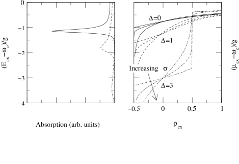
FIG. 1.: Right panel: dependence of the chemical potential on excitation density for detunings $\Delta=0,1$ and $3$ and variances $\sigma=0,0.5$ and $1$. Left panel: absorption spectrum for a microcavity at $\rho_{ex}=-0.5$ and $T=0$ for $\sigma=0.5$ and the same three detunings.

The dependence of $\mu_{ex}$ on $\rho_{ex}$ in the inhomogeneously broadened case is also illustrated in the right panel of Fig. 1. It is qualitatively rather similar to the homogeneous case. Instead of the finite intercept of the homogeneous case we now have $\mu_{ex}\to-\infty$ as $\rho_{ex}\to-0.5$. This behavior is again caused by the tails of the Gaussian distribution. To demonstrate how $\mu_{ex}$ approaches the conventional polariton energy $E_{\mathrm{LPB}}$ in the homogeneous, low-density limit, we compare the behavior of $\mu_{ex}$ with the density of states for the linear-response excitations of the empty($\rho_{ex}=-0.5$) cavity. This density of states is the optical absorption spectrum of the cavity, and is plotted in the left panel of Fig. 1 for $\sigma=0.5$ and $\Delta=0,1$ and $3$. We will describe how it is calculated in section VII. At very low densities, $\mu_{ex}$ lies in the tails of the exciton distribution. With increasing density, these states quickly saturate, producing a sharp rise in $\mu_{ex}$. As $\mu_{ex}$ reaches the polariton peak, the sharp rise in the density of states for the coupled modes produces a kink in the chemical potential. In the homogeneous limit, this kink moves to zero density and corresponds to the usual polariton energy. Since the density of states at this point is infinite in the homogeneous limit, these polaritons are simple bosons.

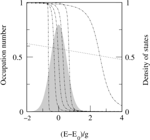
FIG. 2.: Occupation of the two-level oscillators at zero temperature as a function of energy E for $\Delta=3$, $T=0$, $\sigma=0.5$ and densities $\rho_{ex}=-0.4,-0.2,0,0.2,0.4,0.6$(dot-dashed curves, increasing from left to right) and $\rho_{ex}=100$(dotted curve). The shaded region shows the Gaussian distribution of oscillator energies used.

Figure 2 shows the occupation of the two-level oscillators in the polariton condensate, for $\Delta=3,\sigma=0.5$ and various densities. The occupation number of the $n^{th}$ two-level oscillator is

$$\frac{1}{2}(v_{n}^{2}-u_{n}^{2}+1)=\frac{1}{2}\left(1-\frac{\tilde{\varepsilon}_{n}}{|E_{n}|}\right).$$

As is clear from the figure, this is a Fermi step broadened by the interaction with the photons, just as the electronic distribution in a BCS superconductor is a Fermi step broadened by the pairing interaction. The states in the broadened region of the step have a finite dipole moment and are involved in the condensate. The Fermi step moves up through the exciton line as the excitation is increased from $\rho_{ex}=-0.5$ and the low-lying electronic states saturate. At very large densities there are a large number of photons, and the Fermi step is almost completely flat: rather than the electronic system completely saturating in the high density limit, it approaches half filling. This is because the half-filled state maximizes the polarization of the electronic states and hence minimizes the dipole interaction between the excitons and the macroscopically occupied cavity mode.

FIG. 3.: The order parameter $\lambda$ as a function of density, for $\sigma=0.5$ and $\Delta=0$, 1 and 3. $\lambda^{2}$ is the photon number per two-level oscillator in the condensed state.

Careful inspection of Fig. 2 reveals that the broadening of the Fermi step produced by the photons does not increase monotonically with density. This corresponds to a non-monotonic dependence of the field amplitude, $\lambda$, on density. This dependence is illustrated in Fig. 3. The field amplitude is related to the electronic polarization by the first of the equations (13). It is proportional to the electronic polarization and inversely proportional to the separation between the chemical potential and the cavity mode. The electronic polarization depends on the density of states in the vicinity of the chemical potential(Fig. 2); the peak in the density of states at the center of the exciton line produces the peak in Fig. 3.

V Large-N Expansion

The variational approach of sections III and  IV becomes exact in the thermodynamic limit $N\to\infty$. Physically, this is because it corresponds to a mean-field treatment of the interaction between electronic excitations. This interaction, between a large number ($N$) of electronic excitations, is mediated by a small number (one) of cavity modes. In a mean-field treatment of this interaction, each electronic excitation is coupled to the average field produced in the cavity by the other electronic excitations. This becomes exact when there are a large number of electronic excitations contributing to a small number of field modes, since the fluctuations of the field are then negligible.

In this section, we develop a mean-field theory for the thermodynamics of the model (1) from the functional-integral representation of the partition function. In this representation, the partition function can be rigorously evaluated, for large $N$, using a saddle-point analysis [26]. From such an analysis, we derive finite-temperature generalizations of the variational expressions (17–19), thus demonstrating that they are rigorous in the limit of large $N$.

The functional integral techniques used here have previously been used [26, 27] to calculate the partition function and excitation energies in the absence of a constraint on the polariton number of a simplification of the Dicke model. While the Hamiltonian of the model discussed in Refs. [26, 27] is given by (1) with $E_{g}(n)=E_{g}$, the local constraints prohibiting two fermions on the same site, (3), are replaced with a global constraint. In contrast, we retain (3) as local constraints, as well as including a distribution of $E_{g}$ and a constraint on the polariton number.

As in sections III and  IV, we work in a grand-canonical ensemble, using a chemical potential $\mu_{ex}$ to constrain the excitation number. We consider the partition function associated with this ensemble

$$Q={\mathrm{Tr}}\,e^{-{\beta(H-\mu_{ex}L)}}.$$

The coherent-state functional-integral formalism allows us to express $Q$, for the model (1), as the constrained functional integral

$$Q=\int{\cal D}\psi\prod_{n}[{\cal D}\eta_{n}\delta(\bar{\eta}_{n}\eta_{n}-1)]e^{-S},$$

with the action

$$S=\int_{0}^{\beta}d\tau\bar{\psi}(\partial_{\tau}+\tilde{\omega}_{c})\psi+\sum_{n}\bar{\eta}_{n}M_{n}\eta_{n}.$$

We have introduced a Nambu spinor

$$\eta_{n}=\left(\begin{array}[]{c}b_{n}\\ a_{n}\end{array}\right)$$

for each two-level oscillator. The matrix $M_{n}$ is

$$M_{n}=\left(\begin{array}[]{cc}\partial_{\tau}+\tilde{\varepsilon}_{n}&g\psi/\sqrt{N}\\ g\bar{\psi}/\sqrt{N}&\partial_{\tau}-\tilde{\varepsilon}_{n}\end{array}\right).$$

Rescaling the boson field $\psi\to\sqrt{N}\psi$ and transferring the fermionic integrals into the action gives

$$Q=\int{\cal D}\psi|J|e^{-NS_{\rm eff}},$$

with an effective action

$$S_{\rm eff} = \int_{0}^{\beta}d\tau\bar{\psi}(\partial_{\tau}+\tilde{\omega}_{c})\psi-\frac{1}{N}\sum_{n}S_{{\rm f},n},$$ (20)

$$S_{{\rm f},n} = \ln\int{\cal D}\eta_{n}\delta(\bar{\eta}_{n}\eta_{n}-1)e^{-\int_{0}^{\beta}\bar{\eta}_{n}P_{n}\eta_{n}},$$ (21)

in which the $P_{n}$ are the matrix operators $M_{n}$ after rescaling the boson field, and $J$ denotes the trivial Jacobian arising from this rescaling.

A Mean-field equation

For large $N$, the dominant contribution to the partition function $Q$ comes from those functions $\psi_{0}(\tau)$ which minimize the action $S_{\mathrm{eff}}$. Such functions obey the Euler-Lagrange equation. For the action (20), this takes the form

$$(\partial_{\tau}+\tilde{\omega}_{c})\psi_{0}(\tau) = \frac{1}{N}\sum_{n}\left.\frac{\delta S_{{\rm f},n}}{\delta\bar{\psi}}\right|_{\psi(\tau)=\psi_{0}(\tau)}$$ (22)

$$= -\frac{g}{N}\sum_{n}\langle\bar{a}_{n}(\tau)b_{n}(\tau)\rangle,$$ (23)

where the right-hand side of this expression is the polarization of the two-level oscillators in thermal equilibrium driven by an external field $\psi_{0}(\tau)$. This polarization appears because the field $\psi_{0}(\tau)$ modifies the eigenstates [28] of the electronic system. A thermal population of these new eigenstates can correspond to a finite polarization of the original fermions. Equation (23) is a self-consistency condition: the cavity field is driven by the polarization of the fermions, which itself arises from the renormalization of the fermions produced by the photons.

Assuming that the self-consistent field $\psi_{0}(\tau)$ is independent of $\tau$, we can calculate the polarization term on the right of (23) by making a Bogolubov transformation

$$\eta_{n}=\left(\begin{array}[]{cc}\cos(\theta)e^{i\phi}&-\sin(\theta)\\ \sin(\theta)&\cos(\theta)e^{-i\phi}\end{array}\right)\left(\begin{array}[]{c}\delta_{n}\\ \gamma_{n}\end{array}\right)$$ (24)

from the $b_{n}$ and $a_{n}$ fermions to new fermions $\delta_{n}$ and $\gamma_{n}$. This transformation diagonalizes $P_{n}$ when $\phi=\arg\lambda$ and $\tan 2\theta=g|\lambda|/\tilde{\varepsilon}_{n}$. The $\delta_{n}$ and $\gamma_{n}$ quasiparticles then have energies $\pm E_{n}$ respectively, with $E_{n}$ defined by equation (19). Since (24) is a rotation in $\eta$ space, it preserves the single occupancy constraints. Thermally populating the new fermions in accordance with the single occupancy constraint we have

$$\langle\bar{a}_{n}b_{n}\rangle = \frac{1}{2}e^{i\phi}\sin(2\theta)\langle\bar{\delta}_{n}\delta_{n}-\bar{\gamma}_{n}\gamma_{n}\rangle$$ (25)

$$= \frac{1}{2}e^{i\phi}\sin(2\theta)\tanh(\beta E_{n}),$$ (26)

and (23) becomes

$$\tilde{\omega}_{c}\lambda=\frac{g^{2}\lambda}{2N}\sum_{n}\frac{1}{E_{n}}\tanh\left(\beta E_{n}\right).$$ (27)

Equation (27) is the finite-temperature generalization of the variational result (17). This generalization is rather straightforward: we have just acquired $\tanh(\beta E)$ factors describing the thermal occupation of the two-level oscillators.

If we remove the constraint on the polariton number, by setting $\mu_{ex}=0$, and set $E_{g}(n)=E_{g}$, then (27) is the form originally derived by Hepp and Lieb [23] for the unconstrained equilibrium of the Dicke model. In that problem, the existence of a condensate requires

$$\frac{\omega_{c}E_{g}}{g^{2}}<1,$$ (28)

since otherwise (27), with $\mu_{ex}=0$ and $E_{g}(n)=E_{g}$, has only the trivial solution $\lambda=0$. However, it is shown in Refs. [29] and [30] that the $A^{2}$ terms of the minimal-coupling Hamiltonian, neglected in the model (1), modify the inequality (28) in a way which is inconsistent with the Thomas-Kuhn-Reich sum rule. This sum rule requires $\kappa E_{g}/g^{2}>1$, where $\kappa$ is the coupling constant for the $A^{2}$ term, while the modified inequality (28) reads

$$\frac{(\omega_{c}+2\kappa)E_{g}}{g^{2}}<1.$$ (29)

Since this inequality cannot be satisfied, the phase transition in the unconstrained case is an unphysical artifact of the model (1). However, we do not believe that the $A^{2}$ terms prevent condensation in the constrained case, because the inequality corresponding to (29) will be

$$\frac{(\tilde{\omega}_{c}+2\kappa)(E_{g}-\mu_{ex})}{g^{2}}<1,$$

and the parameter $\mu_{ex}$ is not restricted by the sum rule.

B Effect of fluctuations

Let us now consider the effect of small fluctuations $\delta\psi(\tau)$ around the mean-field solution. Expanding $S_{\rm eff}$ to second order in a functional Taylor series around the mean-field solution we have

$$Q\approx e^{-NS_{0}}\int{\cal D}(\delta\psi)|J|e^{-NS_{2}[\delta\psi,\bar{\delta\psi}]}.$$ (30)

Here $S_{0}$ is the action evaluated on the extremal trajectory and $S_{2}$ is the quadratic action from the second order term in the Taylor series. $S_{2}$ is the effective action for small fluctuations of the electromagnetic field. The kernel of $S_{2}$, ${\mathcal{G}}^{-1}$, is the inverse of the thermal Green’s function for the photons.

The integral over fluctuations in (30) contributes a term

$$\frac{1}{N}\ln\det{\mathcal{G}}^{-1}$$

to the free energy density. Since the mean-field solution should be a minimum of the action, the eigenvalues of ${\mathcal{G}}^{-1}$ should be positive. Then $\ln\det{\mathcal{G}}^{-1}$ is finite as $N\to\infty$, there is no fluctuation contribution to the free energy density in this limit, and the mean-field theory becomes exact.

C Effective action for fluctuations

However, we have yet to check whether the solutions to (27) are actually minima of the action or merely extrema, i.e. whether the mean-field solutions are stable against fluctuations. To check this, we will need the effective action $S_{2}$, which we derive in this section.

To obtain $S_{2}$, we calculate the (functional) second derivatives of $S_{\rm eff}$, and evaluate them on the extrema $\psi(\tau)=\psi_{0}(\tau)=\lambda$. In the frequency representation, the components of $S_{2}$ are

$$\frac{\partial^{2}S_{\rm eff}}{\partial{\psi(\omega)}\partial{\bar{\psi}(\omega^{\prime})}}= \beta\delta(\omega^{\prime}-\omega)\bigg{[}i\omega+\tilde{\omega}_{c}$$ (33)

$$-\frac{g^{2}}{N}\sum_{n}\int_{0}^{\beta}e^{-i\omega\tau}(\langle\sigma_{n}^{-}(\tau)\sigma_{n}^{+}(0)\rangle$$

$$\phantom{-\frac{g^{2}}{N}\sum_{n}\int_{0}^{\beta}e^{-i\omega\tau}(}-\langle\sigma_{n}^{-}\rangle\langle\sigma_{n}^{+}\rangle)\bigg{]}d\tau,$$

and

$$\frac{\partial^{2}S_{\rm{eff}}}{\partial{\psi(\omega)}\partial{\psi(\omega^{\prime})}}= -\beta g^{2}\delta(\omega^{\prime}+\omega)$$ (36)

$$\times\frac{1}{N}\sum_{n}\int_{0}^{\beta}e^{i\omega\tau}(\langle\sigma_{n}^{+}(\tau)\sigma_{n}^{+}(0)\rangle$$

$$\phantom{\times\sum_{n}\int_{0}^{\beta}e^{i\omega\tau}(}-\langle\sigma_{n}^{+}\rangle\langle\sigma_{n}^{+}\rangle)d\tau.$$

$\omega$ and $\omega^{\prime}$ denote bosonic Matsubara frequencies, $\sigma_{n}^{+}=b^{\dagger}_{n}a_{n}$ is the polarization operator for the $n^{th}$ two-level oscillator, and the integrands are the susceptibilities of the two-level oscillators in the self-consistent field $\lambda$.

(33) and (36) describe coupled fluctuations of the cavity field and the electronic polarization. They are analogous to the Dyson-Gor’kov-Beliaev equations [26] of the theory of superconductors and weakly-interacting Bose gases. Because we are working with a condensed system there is an anomalous contribution to $S_{2}$, (36), from fluctuations which do not conserve the number of excitations above the condensate, i.e. those in which an excitation enters or leaves the condensate.

To calculate the susceptibilities which appear in (33), we rewrite them in terms of the renormalized two-level oscillators using the transformation (24), transform to the Schrödinger representation, and take thermal and quantum-mechanical averages over the renormalized eigenstates. This gives

$$S_{2}[\delta\psi,\bar{\delta\psi}] = \beta\sum_{\omega}\left(\begin{array}[]{cc}\bar{\delta\psi}(\omega)&\delta\psi(-\omega)\end{array}\right){\mathcal{G}}^{-1}\left(\begin{array}[]{c}\delta\psi(\omega)\\ \bar{\delta\psi}(-\omega)\end{array}\right),$$ (40)

$${\mathcal{G}}^{-1} = \left(\begin{array}[]{cc}K_{1}&K_{2}\\ K_{2}^{\ast}&K_{1}^{\ast}\end{array}\right),$$ (43)

$$K_{1} = i\omega+\tilde{\omega}_{c}+\frac{g^{2}}{N}\sum_{n}\bigg{[}\frac{1}{E_{n}}\tanh\left(\beta E_{n}\right)$$ (45)

$$\times\frac{i\tilde{\varepsilon}_{n}\omega-2\tilde{\varepsilon}_{n}^{2}-g^{2}|\lambda|^{2}}{\omega^{2}+4E_{n}^{2}}+\delta_{\omega}\alpha_{n}|\lambda|^{2}g^{2}\bigg{]},$$

$$K_{2} = \frac{g^{4}\lambda^{2}}{N}\sum_{n}\bigg{[}\frac{1}{E_{n}(\omega^{2}+4E_{n}^{2})}\tanh\left(\beta E_{n}\right)$$ (47)

$$+\delta_{\omega}\alpha_{n}\bigg{]},$$

$$\alpha_{n} = -\frac{\beta}{4E_{n}^{2}}{\rm{sech}}^{2}\left(\beta E_{n}\right).$$ (48)

Note that, for the condensed state, ${\mathcal{G}}^{-1}$ takes different forms at $\omega=0$ and at finite $\omega$. This is because thermal fluctuations at $\omega=0$ include both fluctuations of the order parameter and quasiparticle excitations [31]. Only the latter appear at finite $\omega$. In the normal state, $\lambda=0$, the effective action simplifies to

$$S_{2} = \beta\sum_{\omega}\bar{\delta\psi}(\omega)\Bigg{[}i\omega+\tilde{\omega}_{c}$$ (50)

$$+\frac{1}{N}\sum_{n}\frac{g^{2}i}{\omega-2i\tilde{\varepsilon}_{n}}\tanh\left(\beta\tilde{\varepsilon}_{n}\right)\Bigg{]}\delta\psi(\omega).$$

D Nature of the extrema

We now use the expressions (40–50) to investigate the nature of the extrema when $E_{g}(n)=E_{g}$.

Considering first a condensed solution, $\lambda\neq 0$, we use the extremal equation (27) to eliminate $\frac{1}{E_{n}}\tanh\left(\beta E_{n}\right)$ from the matrix ${\mathcal{G}}^{-1}$. The eigenvalues of the resulting matrix are all strictly positive provided that $\tilde{\omega}_{c}>0$, except for a single zero eigenvalue at $\omega_{n}=0$. From (27) we see that the condensed solutions always have $\tilde{\omega}_{c}>0$. Thus we conclude that, at a condensed solution, the action has a minimum in all but one direction, and is locally flat in this one direction.

We show in Appendix A that the single zero eigenvalue describes a change in the overall phase of the condensate. It is the Goldstone mode corresponding to the broken gauge symmetry of the condensate. Because we are considering a broken symmetry state, we should not integrate over these fluctuations when calculating the partition function. Since the other eigenvalues of ${\mathcal{G}}^{-1}$ are always positive for the condensed solutions, these solutions are stable against physical fluctuations, and the mean-field theory is exact.

Turning now to the normal solution, $\lambda=0$, we find from (50) that this is a minimum of the action unless

$$\tilde{\omega}_{c}<\frac{g^{2}}{2\tilde{\varepsilon}}\tanh(\beta\tilde{\varepsilon}).$$ (51)

This is just the condition for the extremal equation (27) to have a condensed solution. Thus we have the usual scenario of a continuous phase transition: there is a phase boundary (51), at which the normal state becomes unstable and a stable, condensed solution appears.

E Density equation

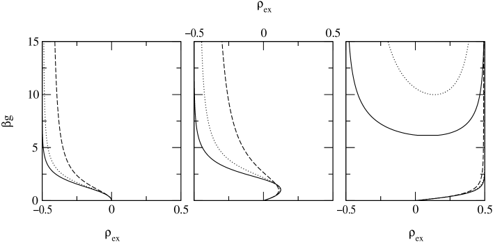
FIG. 4.: Phase boundaries for $\Delta=0$(left panel), $\Delta=1$(center panel) and $\Delta=3$(right panel), and variances $\sigma=0$(solid lines), $\sigma=0.5$(dotted lines) and $\sigma=1$(dashed lines). For $\Delta=3$, $\sigma=1$ the upper branch of the phase boundary lies off the scale, while for $\Delta=3$, $\sigma=0.5$ the lower branch is indistinguishable from the homogeneous case.

As well as the mean-field equation (27), we need the equation relating the density $\rho_{ex}$ to the corresponding chemical potential $\mu_{ex}$. This is obtained from the partition function in the standard way,

$$\rho_{ex}=\frac{1}{\beta N}\frac{\partial}{\partial\mu_{ex}}\ln Q.$$ (52)

The asymptotic form for the partition function is $Q\sim e^{-NS_{0}}$, where $S_{0}$ is the minimal action. Inserting this asymptotic form in (52) gives, for the solution $\psi_{0}(\tau)=\lambda$,

$$\rho_{ex}=|\lambda|^{2}-\frac{1}{2N}\sum_{n}\frac{\tilde{\varepsilon}_{n}}{E_{n}}\tanh\left(\beta E_{n}\right),$$ (53)

which is the generalization of (18) to finite temperatures.

The first term in (53) is the contribution to the excitation density from the macroscopic electromagnetic field, while the second term is the contribution from the thermal population of renormalized electronic excitations. In the absence of a macroscopic electromagnetic field, $\lambda=0$, both the photon contribution and the renormalization of the electronic excitations disappear. The expression (53) is then the familiar form for the excitation of a set of two-level oscillators.

VI Phase diagram

From (51) and (53) we have the critical temperature for condensation, as a function of the excitation density, in the homogeneous model:

$$\beta_{c}g=\frac{4\tanh^{-1}(2\rho_{\mathrm{e}x})}{\Delta\pm\sqrt{\Delta^{2}-8\rho_{\mathrm{e}x}}}.$$ (54)

Note that the transition temperature depends logarithmically on the density, and its scale is set by the interaction strength $g$. This is in contrast with a model of propagating, weakly-interacting bosons, where the transition temperature varies as a power law of the density and its scale is set by the mass of the bosons.

At low densities, (54) is the phase boundary separating a population of electronic excitations with energy $E_{0}$ from a population of conventional polaritons with energy $E_{\mathrm{LPB}}$. To see this, note that such a transition would occur when the chemical potential for the electronic excitations reaches $E_{\mathrm{LPB}}$, corresponding to a density $\rho_{ex}+0.5\approx e^{-\beta_{c}(E_{0}-E_{\mathrm{L}PB})}$, which is the low-density limit of (54).

For the inhomogeneous model, we calculate the phase boundary numerically, assuming the same Gaussian distribution of energies as in section IV. We obtain the critical chemical potential for condensation, $\mu_{c}(\beta_{c})$, by demanding that (27) have a repeated root $\lambda=0$, and then use (53) to obtain the critical density $\rho_{c}(\beta_{c})$.

In Fig. 4 we plot the homogeneous phase boundaries (54), along with numerical results for the inhomogeneous model with $\sigma=0.5$ and 1. On resonance, $\Delta=0$, the transition temperature increases monotonically with density. The system is always condensed for $\rho_{ex}>0$, because to exceed this density would require a chemical potential above the center of the energy distribution of the electronic excitations, and hence above the bosonic cavity mode. While for $\Delta<0$(not illustrated) the phase boundary is qualitatively unchanged from the resonant case, for $\Delta>0$ we find reentrant behavior. This behavior is the result of the saturable nature of the electronic states. It can be understood by considering the limits $\rho_{ex}\to\pm 0.5$ when $\Delta\gg 0$. Near the $\rho_{ex}=-0.5$ limit, the normal state consists of a small number of electronic excitations, weakly interacting with each other through the cavity mode. They condense when their density exceeds a critical value set by the strength of their interaction, which is determined by $\Delta$ and $g$. Near the $\rho_{ex}=0.5$ limit, the electronic system is constrained to be fully occupied, and the normal state consists of a small number of holes in an otherwise completely excited electronic system. These holes again interact through the cavity mode, and so the transition occurs when the density of holes, $0.5-\rho_{ex}$, exceeds a critical value. For $\Delta\to\infty$ the critical densities of holes and excitons are identical, so the phase diagram is symmetric about $\rho=0$. For finite $\Delta$, the interaction is stronger for the holes than for excitons, since they are nearer in energy to the cavity mode, and so the phase boundary becomes skewed to the forms shown.

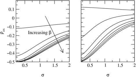
FIG. 5.: Dependence of the critical density on the inhomogeneous broadening $\sigma$, for $\Delta=0$(left panel) and $\Delta=1$(right panel), and $\beta=1$(top curve), 3, 5, 7, 9, 11, 13(lowest curve).

At temperatures which are high compared with the inhomogeneous broadening $\sigma g$, thermal fluctuations dominate over the inhomogeneous broadening. Thus at these temperatures the inhomogeneous broadening has little effect, as can be seen in Fig. 4. However, at low temperatures the inhomogeneous broadening suppresses condensation by increasing the energy separation between the electronic excitations and the photons, collapsing the phase boundaries towards $\rho_{ex}=0$. The effects of inhomogeneous broadening are further illustrated in Fig. 5, which shows the dependence of the critical density on $\sigma$ at various temperatures for detunings $\Delta=0$ and $\Delta=1$.

VII Excitation energies

In this section, we use (40) and (50) to study the excitation spectrum of the quasi-equilibrium states of the model (1). The excitation spectra we calculate explain the form of the phase diagrams in Fig. 4. The excitation spectra of the two quasi-equilibrium states are different from each other, and also from the excitation spectrum of a conventional laser. Since the excitation spectrum is directly related to the optical absorption spectrum of the cavity, which is an experimentally accessible quantity, these spectra offer a clear experimental signature of polariton condensation.

The matrix ${\mathcal{G}}^{-1}$, given by (40), is the inverse of the thermal Green’s function for the photons. We use the standard relations [31, 32] between thermal Green’s functions, retarded Green’s functions, and excitation spectra, to extract the latter from (40).

A Homogeneous model

We begin with the normal state of the homogeneous model. The inverse of the normal state Green’s function contained in (50) can be written as a sum of simple poles

$${\mathcal{G}}(\omega_{n})=\frac{C_{+}}{i\omega_{n}+E_{+}}+\frac{C_{-}}{i\omega_{n}+E_{-}}.$$ (55)

The structure of this Green’s function is clear: we have two excitations, with quasiparticle energies

$$E_{\pm}+\mu_{\mathrm{ex}}=[(\omega_{c}+E_{g})\pm g\sqrt{\Delta^{2}-8\rho_{\mathrm{e}x}}]/2,$$

and corresponding weights

$$C_{\pm}=\pm(2\tilde{\varepsilon}-E_{\pm})/(E_{-}-E_{+}).$$

These normal-state excitations are polaritons in the general sense of Hopfield [2]: coupled modes involving the linear response of the electronic system around its equilibrium state. The gap in the spectrum is increased over the bare detuning $\Delta$ owing to the dipole coupling between the excitons and the cavity mode. The presence of excitation in the ground state, either driven by finite temperatures or by finite $\mu_{\mathrm{e}x}$, causes the two polariton branches to attract. This attraction is due to the decrease in the polarizability of the electronic states as their population increases and saturation occurs. It can also be understood in terms of an angular momentum representation [16] for the collective states of the electronic system. In such a representation, the excitation of the electronic states corresponds to the z component of an angular momentum, while their polarization corresponds to the raising operator $S_{+}$. Thus the polarizability of the electronic states is maximized at $\langle S_{z}\rangle=-N/2$.

Since condensation is a phase transition, we expect a qualitatively different excitation spectrum in the condensed state. From (40) and (27), we find for the leading component of the matrix thermal Green’s function

$${\mathcal{G}}_{11}(i\omega_{n})=\frac{\tilde{\omega}_{c}(\omega^{2}+2g^{2}|\lambda|^{2})-i\omega(\omega^{2}+4E^{2}+2\tilde{\omega}_{c}\tilde{\varepsilon})}{(i\omega_{n})^{2}(i\omega_{n}+\xi)(i\omega_{n}-\xi)(1+\delta_{\omega_{n}}\alpha)},$$ (56)

with $\xi=\sqrt{(\tilde{\omega}_{c}+2\tilde{\varepsilon})^{2}+4g^{2}|\lambda|^{2}}$. The interpretation of this Green’s function is complicated because, as we have already mentioned, it describes both quasiparticle excitations and fluctuations of the order parameter. To rigorously obtain the quasiparticle spectrum, we should extract the contribution to (56) from the order parameter fluctuations, and analytically continue the remainder to obtain the retarded Green’s function. Rather than follow such a procedure, we propose the following physically appealing if mathematically naïve interpretation of (56): the Kronecker delta and the $(i\omega_{n})^{2}$ terms in the denominator describe the condensate response, leaving quasiparticle excitations at energies $\pm\xi$. The $(i\omega_{n})^{2}$ is clearly associated with the phase mode of the condensate, discussed in Appendix A, while the Kronecker delta is related to number fluctuations of the condensate [33]. The excitations at energy $\pm\xi$ are coupled exciton-photon modes in the presence of the macroscopic electromagnetic field of the condensate. $\xi$ is analogous to the pair breaking energy in a superconductor: it is the energy required to extract an exciton-photon complex from the condensate. Note that if we remove the photon contribution to this energy, by setting $\tilde{\omega}_{c}=0$, then $\xi$ becomes the familiar expression [28] for the energy of an electron-hole pair in the presence of a classical electromagnetic field at frequency $\mu_{ex}$.

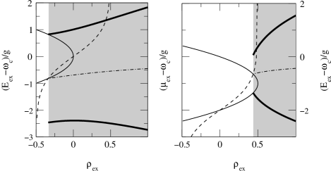
FIG. 6.: Excitation energies and chemical potentials as a function of density for the homogeneous model at $\Delta=0$ (left panel) and $\Delta=2$ (right panel), both with $g\beta=2$. Thin solid lines: normal state excitation energies. Thick solid lines: condensed state excitation energies. Dashed lines: normal state chemical potential. Dot-dashed lines: condensed state chemical potential. The shading marks the condensed region for this $\beta$.

In Fig. 6, we illustrate the evolution of the excitation energies of the microcavity with increasing density. To explain the relationship between the excitation energies and the phase diagram, we also plot the chemical potentials for the normal and condensed states on this figure. The left panel of this figure should be compared to the $g\beta=2$ line of the corresponding phase diagram, which is the left panel of Fig. 4. When $\Delta=0$ and $\rho_{\mathrm{e}x}=-0.5$ the system is in the normal state. Increasing $\rho_{\mathrm{e}x}$ populates the electronic excitations, increasing the chemical potential and decreasing the polariton splitting. Eventually the chemical potential crosses the lower polariton branch from below and the system condenses. At the critical density, the lower polariton branch joins to the phase mode at the chemical potential, the upper branch joins to the “pair breaking” excitation, and an excitation appears below the chemical potential. This latter excitation has zero weight at the transition. It corresponds to an excited state to ground state transition, where an exciton-photon complex is absorbed into the condensate. There is no corresponding excitation in the normal state Green’s function, because the ground state of the $N+1$ particle system($N+1$ excitons) cannot be reached from the excited states of the $N$ particle system($N-1$ excitons and 1 polariton) by adding a photon.

The relationship between the excitation spectrum and the phase diagram is slightly different when the transition occurs for $\rho_{ex}>0$. For example, in the right panel of Fig. 6 the chemical potential crosses the lower polariton branch at $\rho_{\mathrm{e}x}=0$ without the condensate appearing. It is not until the chemical potential crosses the upper polariton branch that the transition occurs. This can be understood by considering the signs of the quasiparticle weights $C_{\pm}$. A positive quasiparticle weight corresponds to absorption of an external field(a particle-like transition), whereas a negative quasiparticle weight corresponds to gain(a hole-like transition). For $\rho_{\mathrm{e}x}>0$, the lower polariton branch has a negative weight: it has become hole-like, and must be below the chemical potential for stability. At the transition it is now this lower branch which joins to the “pair forming” excitation of the condensate, while the upper branch joins to the phase mode and the “pair breaking” excitation appears above the phase mode.

B Inhomogeneous model

Since the inhomogeneous model has a distribution of excitations, we must study the spectral function $A(\omega)$. $A(\omega)$ is proportional to the imaginary part of the retarded Green’s function,

$$A(\omega)=2\Im G^{R}(-\omega+\mu_{ex}).$$ (57)

It is proportional to the optical absorption coefficient of the cavity at frequency $\omega$, i.e. the imaginary part of the dielectric susceptibility.

To obtain $A(\omega)$ we require the retarded Green’s function $G^{R}$. In the normal state this is given by the straightforward analytical continuation

$$G^{R}(\omega)=\lim_{\eta\to 0^{+}}{\mathcal{G}}(i\omega_{n}=\omega-i\eta).$$ (58)

However, in the condensed state we face the problem, already mentioned for the homogeneous case, of separating the order parameter response from the quasiparticle response. We circumvent this problem by simply assuming that the continuation (58) of the normal state Green’s function also applies in the condensed state.

Inverting the ${\mathcal{G}}^{-1}$ contained in (40) and using (57) and (58) expresses $A(\omega)$ in terms of integrals over the distribution of energies of the two-level oscillators. We evaluate these integrals in the limit $\eta\to 0$ by setting $\eta=0$ in the integrands and deforming the contour of integration around the poles of the integrand on the real axis. The contribution to the integrals from the detour around the poles can be performed analytically, leaving a principal value integral which we evaluate numerically.

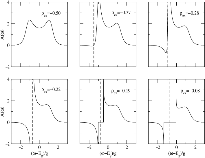
FIG. 7.: Spectral functions(optical absorption spectra) $A(\omega)$, for $\Delta=0$, $g\beta=2$, $\sigma=1$ and chemical potentials $(\mu_{ex}-E_{g})/g=-5,-1.5,-1.0,-0.76,-0.75,-0.70$, increasing from top left to bottom right through the transition at $(\mu_{ex}-E_{g})/g=-0.76$. The top row of plots are in the normal state, the bottom left hand plot at the transition and the remaining plots in the condensed state. The vertical dashed lines mark the chemical potential.

Figure 7 shows the evolution of our calculated absorption spectra, $A(\omega)$, as we increase the density through the transition, for $g\beta=2$, $\sigma=1$, and $\Delta=0$. The corresponding chemical potential is marked as the dashed line. For the empty cavity, $\rho_{ex}=-0.5$, we recover the absorption spectrum calculated by Houdré et al. [34]. Comparison with Fig. 6 shows that, for these parameters, the positions of the polariton peaks are largely unaffected by the inhomogeneous broadening. However, since the polaritons are now resonant with a significant density of electronic states they become broadened. Increasing the chemical potential, but remaining in the normal state, we see the thermal occupation factors producing gain below the chemical potential and increased absorption just above. The collapse of the polariton splitting evident in Fig. 6 is hardly noticeable at these low densities. As the density is increased still further a pole appears in $A(\omega)$ at the chemical potential; this marks the onset of condensation. Above the critical density the coherent cavity field, oscillating at frequency $\mu_{ex}$, produces a gap of magnitude $4g|\lambda|$ in the spectrum. The peak on the high energy side of the gap connects smoothly to the upper polariton peak of the normal state, just as in the homogeneous case. In the homogeneous case we noted the appearance of an excitation below the chemical potential as we crossed the transition. This is still present in the inhomogeneous case, but for the parameters used in Fig. 7 it is far too weak to be visible.

VIII Conclusions

Real microcavities are far more complex than the idealized model (1). However, like our model, they consist of photons coupled to electronic excitations which are bosons at low densities, but reveal their fermionic internal structure at high densities. We have shown how the polariton condensate may be generalized to allow for the saturation nonlinearity produced by such fermionic structure. The saturation nonlinearity can produce (1)a collapse of the splitting between the peaks in the absorption spectrum of the normal state with increasing density, (2)a shift of the chemical potential of the condensate away from the conventional polariton energy, and (3)an unusual reentrant phase boundary for condensation.

Experimental work on cavity polaritons has concentrated on microcavities containing high-quality GaAs quantum wells. In these systems, the excitons are weakly-bound, and rather delocalized. Thus, while the saturation nonlinearity discussed here is present for these excitations, it will be accompanied by other nonlinearities produced by the overlap of the wavefunctions of different excitons and the ionization of excitons [35, 36]. These effects may well prevent condensation, but are separated from the saturation nonlinearity considered here in systems with localized, tightly-bound excitons. Note also that tightly-bound excitons have a large dipole coupling $g$, and hence the transition temperature will be larger.

For real examples of localized oscillators, there will be some energy $E_{m}$ above which delocalized states exist. The picture of a condensate formed from localized oscillators then only holds when $E_{m}-\mu_{ex}$ is large compared with $\beta^{-1}$ and $g$. By considering Fig. 6, we deduce that to completely realize a reentrant phase diagram like that shown in Fig. 4 requires an energy gap $\Delta E$ separating the localized and delocalized excitations; this gap must be large compared with $g$ and $\beta^{-1}$. Such a gap could occur in organic semiconductors [6, 7]. In these systems, excitons are strongly bound and therefore small(Frenkel). They readily self-trap on local lattice distortions and on impurities in these, often highly disordered, materials. An energy gap $\Delta E$ could exist in inorganic quantum wells if the excitons move in a potential containing deep, well-separated traps, perhaps associated with interface islands in narrow quantum wells [37, 38, 39].

The disordered quantum wells studied by Hegarty et al. [40] provide an example of a system without a gap separating the localized and delocalized excitations. These systems show a single inhomogeneously broadened exciton line, unlike the quantum wells of Refs. [37, 38, 39]. The “mobility edge” $E_{m}$ lies near to the center of the exciton line. One may be able to form a condensate which does not involve delocalized excitations using this type of quantum well if the inhomogeneous broadening is large compared with $g$ and $\beta$ and the cavity mode is placed low down in the exciton line. The transition would then occur when the chemical potential is well separated from $E_{m}$.

The polariton condensate described here is formed from a quasi-thermal population of electronic excitations which are renormalized by the coherent photons in the cavity. This renormalization, embodied in the Bogolubov transformation (24), produces a gap of magnitude $4g|\lambda|$ in the absorption spectrum of the condensate. Such renormalizations, and hence the gap, are absent in conventional semiconductor lasers [41], for which a quasi-thermal population of the bare electronic excitations is assumed. Thus the presence or absence of a gap allows the polariton condensate to be distinguished from a conventional laser.

In a conventional laser, the renormalization of the electronic excitations by the photons, and hence the gap, is absent because the electronic polarization is very heavily damped. The destruction of a gap by damping is well-known in superconductors, where it is associated with magnetic impurities. Such impurities suppress the gap, eventually to zero. The destruction of the gap does not coincide with the destruction of the order parameter however: near to $T_{c}$ there is a regime of gapless superconductivity, in which there is an order parameter but no gap in the single-particle spectrum. This regime should correspond to the conventional semiconductor laser, although the actual damping mechanisms will differ.

The non-equilibrium analog [42] of the crossover illustrated in Fig. 6 and Fig. 7, from a two-peaked polariton spectrum to a “Stark triplet”, has been observed experimentally [43]. In that experiment, the gapped absorption spectrum is observed simultaneously with the excitation pulse. Thus there is no thermalization involved in producing the gapped spectrum. It is the result of coherence in the excitation pulse, rather than the spontaneous coherence of condensation. Nonetheless, these experiments demonstrate the renormalization of the electronic states that is essential in the polariton condensate.

To reach the quasi-equilibrium regime we have described requires a system where the polariton lifetime is long compared with the time required to reach thermal equilibrium at a fixed number of polaritons. Current semiconductor microcavities have lifetimes for the photons, and hence the polaritons, of the order of picoseconds. Finding an exciton system which thermalizes on this timescale may be difficult. However, there seems no reason to suppose it is impossible, particularly beyond the linear regime, since nonlinearities can enhance relaxation [10]. Furthermore, microcavities are available with lifetimes far greater than picoseconds. For example, silica microspheres have confined modes with lifetimes of microseconds [44].

IX Acknowledgments

This work was supported by the Engineering and Physical Sciences Research Council, U.K.

A The phase mode

In this appendix we investigate the zero eigenvalue of ${\mathcal{G}}^{-1}$ that appeared while studying the stability of the condensate in the homogeneous case. We first prove that the zero is also present in the inhomogeneous model, and that it describes phase fluctuations of the condensate. It is thus the Goldstone mode reflecting the degeneracy of the ground state with respect to the phase of the order parameter. We then argue that the zero eigenvalue does not contribute to the free energy density in the thermodynamic limit. Although the physics we discuss in this appendix is well understood in general, it is particularly transparent in our simple model.

We note that, at $\omega=0$, $K_{1}$ is real and positive. The eigenvalues of ${\mathcal{G}}^{-1}$ are then $K_{1}\pm|K_{2}|$. Since from the explicit forms of $K_{1}$, $K_{2}$ and the extremal equation (27) we have $|K_{2}|=K_{1}$, as required in general by the Hugenholtz-Pines relation [26, 45], ${\mathcal{G}}^{-1}$ has a zero eigenvalue.

To illustrate that the zero eigenvalue is the phase mode of the condensate, note that since $\arg K_{2}=2\arg\lambda=2\phi$ we can write

$${\mathcal{G}}^{-1}\propto\left(\begin{array}[]{cc}1&e^{2i\phi}\\ e^{-2i\phi}&1\end{array}\right).$$

The eigenvector of this matrix with zero eigenvalue is perpendicular in the complex plane to the order parameter $\lambda$.

Since we are considering a broken symmetry system, we should not include states with different phases of the order parameter when calculating the partition function. Thus on physical grounds, we should discard the zero mode when computing the partition function.

A formal approach which allows calculations in the presence of the zero eigenvalue is to introduce symmetry breaking terms which are taken to zero after the thermodynamic limit. This is the standard method for applying statistical mechanics to broken symmetry systems [32]. The appropriate symmetry breaking terms for a Bose condensed system pin the phase of the order parameter. They are sources and sinks for the photons, and appear in the effective action $S_{\mathrm{e}ff}$ as $\frac{1}{\sqrt{N}}\left(\bar{\psi}J+\bar{J}\psi\right).$ These terms do not contribute directly to (40), but appear as a source term in (27). The original zero eigenvalue of ${\mathcal{G}}^{-1}$ is now $K_{1}-|K_{2}|=-J/(\psi_{0}\sqrt{N})$. Since for the equilibrium solution we must have $\phi-\arg J=\pi$, the contribution of the original zero eigenvalue to the free energy density is proportional to

$$\lim_{J\to 0}\lim_{N\to\infty}\frac{1}{N}\ln\left(\frac{|J|}{|\lambda|\sqrt{N}}\right)=0.$$

REFERENCES

- [1] C. F. Klingshirn, Semiconductor Optics (Springer, Berlin, 1997).
- [2] J. J. Hopfield, Phys. Rev. 112, 1555 (1958).
- [3] M. G. Raizen et al., Phys. Rev. Lett. 63, 240 (1989).
- [4] C. Weisbuch, M. Nishioka, A.Ishikawa, and Y.Arakawa, Phys. Rev. Lett. 69, 3314 (1992).
- [5] A. Tedicucci et al., Phys. Rev. Lett. 75, 3906 (1995).
- [6] D. G. Lidzey et al., Nature 395, 53 (1998).
- [7] D. G. Lidzey et al., Phys. Rev. Lett. 82, 3316 (1999).
- [8] R. Rapaport et al., Phys. Rev. Lett. 84, 1607 (2000).
- [9] L. V. Keldysh, in Bose-Einstein Condensation, edited by A. Griffin, D. W. Snoke, and A. Stringari (Cambridge University Press, Cambridge, U.K., 1995).
- [10] P. Senellart and J. Bloch, Phys. Rev. Lett. 82, 1233 (1999).
- [11] L. S. Dang et al., Phys. Rev. Lett. 81, 3920 (1998).
- [12] V. Pellegrini, R. Colombelli, L. Sorba, and F. Beltram, Phys. Rev. B 59, 10059 (1999).
- [13] P. G. Savvidis et al., Phys. Rev. Lett. 84, 1547 (2000).
- [14] R. M. Stevenson et al., Phys. Rev. Lett. 85, 3680 (2000).
- [15] P. Nozières, in Bose-Einstein Condensation, edited by A. Griffin, D. W. Snoke, and A. Stringari (Cambridge University Press, Cambridge, U.K., 1995), pp. 15–30.
- [16] R. H. Dicke, Phys. Rev. 93, 99 (1954).
- [17] P. R. Eastham and P. B. Littlewood, Solid State Commun. 116, 357 (2000).
- [18] L. Allen and J. H. Eberly, Optical Resonance and Two-level Atoms (Dover, New York, 1975).
- [19] M. O. Scully and M. S. Zubairy, Quantum Optics (Cambridge University Press, Cambridge, U.K., 1997).
- [20] J. Bloch et al., Physica E 2, 915 (1998).
- [21] J.–M. Gérard and B. Gayral, in Confined Photon Systems, Lecture Notes in Physics, edited by H. Benisty et al. (Springer, Berlin, 1999), pp. 331–351.
- [22] P. R. Eastham, Ph.D. thesis, Cambridge University, 2000.
- [23] K. Hepp and E. H. Lieb, Ann. Phys. 76, 360 (1973).
- [24] V. F. Elesin and Y. V. Kopaev, Pism’a Zh. Eksp. Teor. Fiz. 24, 78 (1976), [JETP Lett. 24(2), 66–69].
- [25] C. Comte and P. Nozières, J. Phys. (Paris) 43, 1069 (1982).
- [26] V. N. Popov and V. S. Yarunin, Collective Effects in Quantum Statistics of Radiation and Matter (Kluwer Academic Publishers, Dordrecht, 1988).
- [27] V. B. Kir’yanov and V. S. Yarunin, Toer. Matematicheskaya Fiz. 43, 91 (1980), [Theoretical and Mathematical Physics 43(1), 340–345].
- [28] V. M. Galitskii, S. P. Goreslavskii, and V. F. Elesin, Zh. Eksp. Teor. Fiz. 30, 207 (1969), [Sov. Phys. JETP 30(1), 117–122].
- [29] K. Rza̧żewski, K. Wódkiewicz, and W. Żakowicz, Phys. Lett. 58A, 211 (1976).
- [30] K. Rza̧żewski, K. Wódkiewicz, and W. Żakowicz, Phys. Rev. Lett. 35, 432 (1975).
- [31] Hydrodynamic Fluctuations, Broken Symmetry and Correlation Functions, No. 47 in Frontiers in Physics, edited by D. Forster (W. A. Benjamin, Inc., Reading, Massachusetts, 1975).
- [32] J. W. Negele and H. Orland, Quantum Many-Particle Systems (Addison-Wesley, Redwood City, California, 1988).
- [33] P. B. Littlewood and C. M. Varma, Phys. Rev. B 26, 4883 (1982).
- [34] R. Houdré, R. P. Stanley, and M. Ilegems, Phys. Rev. A 53, 2711 (1996).
- [35] R. Houdré et al., Phys. Rev. B 52, 7810 (1995).
- [36] F. Jahnke et al., Phys. Rev. Lett. 77, 5257 (1996).
- [37] D. Gammon et al., Phys. Rev. Lett. 76, 3005 (1996).
- [38] H. F. Hess et al., Science 264, 1740 (1994).
- [39] N. H. Bonadeo et al., Phys. Rev. Lett. 81, 2759 (1998).
- [40] J. Hegarty, L. Goldner, and M. D. Sturge, Phys. Rev. Lett. 30, 7346 (1984).
- [41] G. P. Agrawal and N. K. Dutta, Semiconductor Lasers, 2nd ed. (Van Nostrand Reinhold, New York, 1993).
- [42] S. Schmitt-Rink, D. S. Chemla, and H. Haug, Phys. Rev. B 37, 941 (1988).
- [43] F. Quochi et al., Phys. Rev. Lett. 80, 4733 (1998).
- [44] V. B. Braginsky, M. L. Gorodetsky, and V. S. Ilchenko, Phys. Lett. A 137, 393 (1989).
- [45] N. M. Hugenholtz and D. Pines, Phys. Rev. 116, 489 (1959).