Vortices in a trapped dilute Bose-Einstein condensate

Abstract

We review the theory of vortices in trapped dilute Bose-Einstein condensates and compare theoretical predictions with existing experiments. Mean-field theory based on the time-dependent Gross-Pitaevskii equation describes the main features of the vortex states, and its predictions agree well with available experimental results. We discuss various properties of a single vortex, including its structure, energy, dynamics, normal modes and stability, as well as vortex arrays. When the nonuniform condensate contains a vortex, the excitation spectrum includes unstable (“anomalous”) mode(s) with negative frequency. Trap rotation shifts the normal-mode frequencies and can stabilize the vortex. We consider the effect of thermal quasiparticles on vortex normal modes as well as possible mechanisms for vortex dissipation. Vortex states in mixtures and spinor condensates are also discussed.

Contents

toc

I Introduction

The recent dramatic achievement of Bose-Einstein condensation in trapped alkali-metal gases at ultra-low temperatures [1, 2, 3] has stimulated intense experimental and theoretical activity. The atomic Bose-Einstein condensates (BECs) differ fundamentally from the helium BEC in several ways. First, BECs in helium are uniform. In contrast, the trapping potential that confines an alkali-metal-atom vapor BEC yields a significantly nonuniform density. Another difference is that in bulk superfluid ⁴He, measurements of the momentum distribution have shown that the low-temperature condensate fraction is $\sim 0.1$, with the remainder of the particles in finite momentum states [4, 5], whereas the low-temperature atomic condensates can be prepared with essentially all atoms in the Bose condensate. Finally, the condensates of alkali vapors are pure and dilute (with mean particle density $\bar{n}$ and $\bar{n}|a|^{3}\ll 1$), so that the interactions can be accurately parametrized in terms of a scattering length $a$ (in current experiments, alkali-metal-atom BECs are much less dense than air at normal pressure). This situation differs from superfluid ⁴He, where the relatively high density and strong repulsive interactions greatly complicate the analytical treatments. As a result, a relatively simple nonlinear Schrödinger equation (the Gross-Pitaevskii equation) gives a precise description of the atomic condensates and their dynamics (at least at low temperatures). One should mention, however, that unlike the spinless ⁴He atoms, alkali atoms have nonzero hyperfine spins, and various forms of spin-gauge effects can be important [6].

Bulk superfluids are distinguished from normal fluids by their ability to support dissipationless flow. Such persistent currents are intimately related to the existence of quantized vortices, which are localized phase singularities with an integer topological charge. The superfluid vortex is an example of topological defects that are well known in liquid helium [7, 8] and in superconductors [9]. The occurrence of quantized vortices in superfluids has been the object of fundamental theoretical and experimental work [10, 11, 12, 13, 14]. Vortex-like excitations exist in the earth’s atmosphere [15], in superfluid hadronic matter (neutron stars) [16], and even in rotating nuclei [17]. Examples of other topological defects that could exist in dilute gas condensates are “textures” found in Fermi superfluid ³He [18], skyrmions [19, 20] and spin monopoles [21]. Vortices in the $A$ and $B$ phases of ³He are discussed in detail in the review articles [22, 23]. In superfluid ³He the Cooper pairs have both orbital and spin angular momentum. These internal quantum numbers imply a rich phase diagram of allowed vortex structures, including nonquantized vortices with continuous vorticity (see also Refs. [24, 25]).

In the framework of hydrodynamics, the vortices obtained from the Gross-Pitaevskii (GP) equation are analogous to vortices in classical fluids [26]. Also the GP equation provides an approximate description of some aspects of superfluid behavior of helium, such as the annihilation of vortex rings [27], the nucleation of vortices [28], and vortex-line reconnection [29, 30].

The initial studies of trapped Bose condensates concentrated on measuring the energy and condensate fraction, along with the lowest-lying collective modes and quantum-mechanical interference effects (see, for example, Ref. [31]). Although the possibility of trapped quantized vortices was quickly recognized [32], successful experimental verification has taken several years [33, 34, 35, 36, 37]. This review focuses on the behavior of quantized vortices in trapped dilute Bose condensates, emphasizing the qualitative features along with the quantitative comparison between theory and experiment.

The plan of the paper is the following. In Sec. II we discuss the basic formalism of mean-field theory (the time-dependent Gross-Pitaevskii equation) that describes dilute Bose-Einstein condensates in the low-temperature limit. We summarize properties of vortices in a uniform condensate and also introduce relevant length and energy scales of a condensate in a harmonic trap. In Sec. III we discuss the structure of stationary vortex states in trapped condensates. We analyze the energy of a straight vortex as a function of displacement from the trap center and consider conditions of vortex stability when the trap rotates. Also we discuss the recent experimental creation of a single vortex and vortex arrays. In Sec. IV we introduce the concept of elementary excitations (the Bogoliubov equations) and analyze the lowest (unstable) mode of the vortex for different values of the interaction parameter. We also consider the splitting of the condensate normal modes due to presence of a vortex line.

In Sec. V we investigate the general dynamical behavior of a vortex, based on a time-dependent variational analysis and on the method of matched asymptotic expansions. The latter method allows us take into account effects of both nonuniform condensate density and vortex curvature. We consider normal modes of a vortex in two- and three-dimensional condensates. Also we discuss the energy of a curved vortex line and a nonlinear tilting of a vortex in slightly anisotropic condensates. In Sec. VI we analyze the effect of thermal quasiparticles on the vortex normal modes and discuss possible mechanisms of vortex dissipation. Also we discuss the influence of vortex generation on energy dissipation in superfluids. In Sec. VII we consider vortices in multicomponent condensates and analyze various spin-gauge effects. In particular, we focus on the successful method of vortex generation in a two-component system that was recently used by the JILA group to create a vortex. In Sec. VIII we draw our conclusions and discuss perspectives in the field.

II Time-dependent Gross-Pitaevskii equation

Bogoliubov’s seminal treatment [38] of a uniform Bose gas at zero temperature emphasized the crucial role of (repulsive) interactions both for the structure of the ground state and for the existence of superfluidity. Subsequently, Gross [39, 40] and Pitaevskii [41] independently considered an inhomogeneous dilute Bose gas, generalizing Bogoliubov’s approach to include the possibility of nonuniform states, especially quantized vortices.

An essential feature of a dilute Bose gas at zero temperature is the existence of a macroscopic wave function (an “order parameter”) $\Psi$ that characterizes the Bose condensate. For a uniform system with $N$ particles in a stationary box of volume $V$, the order parameter $\Psi=\sqrt{N_{0}/V}$ reflects the presence of a macroscopic number $N_{0}$ of particles in the zero-momentum state, with the remaining $N^{\prime}=N-N_{0}$ particles distributed among the various excited states with ${\bf k}\neq 0$. The single-particle states for periodic boundary conditions are plane waves $V^{-1/2}e^{i{\bf k\cdot r}}$ labeled with the wave vector ${\bf k}$, and the corresponding creation and annihilation operators $a_{{\bf k}}^{\dagger}$ and $a_{{\bf k}}$ obey the usual Bose-Einstein commutation relations $[a_{{\bf k}},a_{{\bf k^{\prime}}}^{\dagger}]=\delta_{{\bf k,k^{\prime}}}$. In the presence of a uniform Bose condensate with ${\bf k}=0$, the ground-state expectation value $\langle a_{0}^{\dagger}a_{0}\rangle_{0}=N_{0}$ is macroscopic, whereas the ground-state expectation value of the commutator of these zero-mode operators $\langle[a_{0},a_{0}^{\dagger}]\rangle_{0}$ necessarily equals 1. Hence the commutator is of order $1/\sqrt{N_{0}}$ relative to each separate operator, and they can be approximated by classical numbers $a_{0}\approx a_{0}^{\dagger}\approx\sqrt{N_{0}}$. This “Bogoliubov” approximation identifies these classical fields as the order parameter for the stationary uniform condensate. In contrast, the ground-state expectation value for all the other normal modes $\langle a_{{\bf k}}^{\dagger}a_{{\bf k}}\rangle_{0}$ is of order unity, and the associated operators $a_{{\bf k}}^{\dagger}$ and $a_{{\bf k}}$ require a full quantum-mechanical treatment.

The existence of nonuniform states of a dilute Bose gas can be understood by considering a second-quantized Hamiltonian

$$\hat{H}=\int dV\left[\hat{\psi}^{\dagger}\left(T+V_{{\rm tr}}\right)\hat{\psi}+\frac{1}{2}g\hat{\psi}^{\dagger}\hat{\psi}^{\dagger}\hat{\psi}\hat{\psi}\right],$$ (1)

expressed in terms of Bose field operators $\hat{\psi}({\bf r})$ and $\hat{\psi}^{\dagger}({\bf r})$ that obey Bose-Einstein commutation relations

$$[\hat{\psi}({\bf r}),\hat{\psi}^{\dagger}({\bf r}^{\prime})]=\delta({\bf r-r}^{\prime}),\quad[\hat{\psi}({\bf r}),\hat{\psi}({\bf r}^{\prime})]=[\hat{\psi}^{\dagger}({\bf r}),\hat{\psi}^{\dagger}({\bf r}^{\prime})]=0.$$ (2)

Here $T=-\hbar^{2}\nabla^{2}/2M$ is the kinetic energy operator for the particles of mass $M$, $V_{{\rm tr}}({\bf r})$ is an external (trap) potential, and the interparticle potential has been approximated by a short-range interaction $\approx g\,\delta({\bf r-r}^{\prime})$, where $g$ is a coupling constant with the dimensions of energy $\times$ volume. For a dilute cold gas, only binary collisions at low energy are relevant, and these collisions are characterized by a single parameter, the $s$-wave scattering length $a$, independent of the details of the two-body potential. An analysis of the scattering by such a potential (see, for example [42, 43]) shows that $g\approx 4\pi a\hbar^{2}/M$. Determinations of the scattering length for the atomic species used in the experiments on Bose condensation give: $a=2.75$ nm for ²³Na [44], $a=5.77$ nm for ⁸⁷Rb [45], and $a=-1.45$ nm for ⁷Li [46]. In a uniform bulk system, $a$ must be positive to prevent an instability leading to a collapse, but a Bose condensate in an external confining trap can remain stable for $a<0$ as long as the number of condensed atoms $N_{0}$ remains below a critical value $N_{cr}\sim d/|a|$, where $d$ is the oscillator length [31, 43]. If the interparticle potential is attractive ($a<0$), the gas tends to increase its density in the trap center to lower the interaction energy. The kinetic energy opposes this tendency, and the resulting balance can stabilize inhomogeneous gas. A vortex line located along the trap axis reduces the peak central density in the cloud of atoms. Thus a vortex can help stabilize a larger trapped condensate with attractive interactions in the sense it can contain a larger number of atoms [47].

The time-dependent Heisenberg operator $\hat{\psi}({\bf r},t)=\exp(i\hat{H}t/\hbar)\,\hat{\psi}({\bf r})\,\exp(-i\hat{H}t/\hbar)$ obeys the equation of motion $i\hbar\,\partial\hat{\psi}({\bf r},t)/\partial t=[\hat{\psi}({\bf r},t),\hat{H}]$, which yields a nonlinear operator equation

$$i\hbar\,\frac{\partial\hat{\psi}({\bf r},t)}{\partial t}=\left(T+V_{{\rm tr}}\right)\hat{\psi}({\bf r},t)+g\,\hat{\psi}^{\dagger}({\bf r},t)\,\hat{\psi}({\bf r},t)\,\hat{\psi}({\bf r},t).$$ (3)

The macroscopic occupation of the condensate makes it natural to write the field operator as a sum $\hat{\psi}({\bf r},t)=\Psi({\bf r},t)+\hat{\phi}({\bf r},t)$ of a classical field $\Psi({\bf r},t)$ that characterizes the macroscopic condensate and a quantum field $\hat{\phi}({\bf r},t)$ referring to the remaining noncondensed particles. To leading order, the Bogoliubov approximation omits the quantum fluctuations entirely, giving the time-dependent Gross-Pitaevskii (GP) equation [39, 41]

$$i\hbar\,\frac{\partial\Psi({\bf r},t)}{\partial t}=\left[T+V_{{\rm tr}}+g\,|\Psi({\bf r},t)|^{2}\right]\Psi({\bf r},t)$$ (4)

for the condensate wave function $\Psi({\bf r},t)$. Since $\hat{\psi}({\bf r},t)$ reduces the number of particles by one, its off-diagonal matrix element $\langle N-1|\hat{\psi}({\bf r},t)|N\rangle$ oscillates at a frequency corresponding to the chemical potential $\mu\approx E_{0}(N)-E_{0}(N-1)$ associated with removing one particle from the ground state. Thus the stationary solutions take the form $\Psi({\bf r},t)=\Psi({\bf r})\,e^{-i\mu t/\hbar}$, where $\Psi({\bf r})$ obeys the stationary GP equation (frequently identified as a nonlinear Schrödinger equation, although the eigenvalue $\mu$ is not the energy per particle)

$$(T+V_{{\rm tr}}+g|\Psi|^{2})\Psi=\mu\Psi.$$ (5)

Apart from very recent work on ⁸⁵Rb using a Feshbach resonance to tune $a$ to large positive values [48], essentially all studies of trapped atomic gases involve the dilute limit ($\bar{n}|a|^{3}\ll 1$, where $\bar{n}$ is the average density of the gas), so that depletion of the condensate is small with $N^{\prime}=N-N_{0}\propto\sqrt{\bar{n}|a|^{3}}N\ll N$. Typically $\bar{n}|a|^{3}$ is always less than $10^{-3}$. Hence most of the particles remain in the condensate, and the difference between the condensate number $N_{0}$ and the total number $N$ can usually be neglected. In this case, the stationary GP equation (5) for the condensate wave function follows by minimizing the Hamiltonian functional

$$H=\int dV\left[\Psi^{*}\left(T+V_{{\rm tr}}\right)\Psi+\frac{1}{2}g|\Psi|^{4}\right],$$ (6)

subject to a constraint of fixed condensate number $N_{0}=\int dV\,|\Psi|^{2}\approx N$ (readily included with a Lagrange multiplier that is simply the chemical potential $\mu$).

A Unbounded Condensate

The nonlinear Schrödinger equation (5) contains a local self-consistent Hartree potential energy $V_{H}({\bf r})=g|\Psi({\bf r})|^{2}$ arising from the interaction with the other particles at the same point. In an unbounded condensate with $V_{{\rm tr}}=0$, the left-hand side of Eq. (5) involves both the kinetic energy $T$ and this repulsive Hartree potential $g|\Psi|^{2}=gn$ for a uniform medium with bulk density $n$. On dimensional grounds, the balance between these two terms implies a “correlation” or “healing” length

$$\xi=\frac{\hbar}{\sqrt{2Mng}}=\frac{1}{\sqrt{8\pi na}}.$$ (7)

This length characterizes the distance over which the condensate wave function heals back to its bulk value when perturbed locally (for example, at a vortex core, where the density vanishes).

For a uniform system in a box of volume $V$, the condensate wave function is $\Psi=\sqrt{N_{0}/V}\approx\sqrt{N/V}$, and Eq. (6) shows that the ground-state energy $E_{0}$ arises solely from the repulsive interparticle energy of the condensate $E_{{\rm int}}\approx\frac{1}{2}\,gN^{2}/V$. The bulk chemical potential is then given by

$$\mu=\left(\frac{\partial E_{0}}{\partial N}\right)_{\!\!V}=gn=\frac{4\pi a\hbar^{2}n}{M}.$$ (8)

The corresponding pressure follows from the thermodynamic relation

$$p=-\left(\frac{\partial E_{0}}{\partial V}\right)_{\!\!N}=\frac{1}{2}gn^{2}=\frac{E_{{\rm int}}}{V}.$$ (9)

Finally, the compressibility determines the bulk speed of sound $s$:

$$s^{2}=\frac{1}{M}\,\left(\frac{\partial p}{\partial n}\right)=\frac{gn}{M}=\frac{\mu}{M}=\frac{4\pi a\hbar^{2}n}{M^{2}},\>\>\hbox{or, equivalently,}\>\>s=\frac{\hbar}{\sqrt{2}M\xi}\,;$$ (10)

Equations (7) and (10) both indicate that a bulk uniform Bose condensate requires a repulsive interaction ($a>0$), since otherwise the healing length and the speed of sound become imaginary.

B Quantum-Hydrodynamic Description of the Condensate

It is often instructive to represent the condensate wave function in an equivalent “quantum-hydrodynamic” form

$$\Psi({\bf r},t)=|\Psi({\bf r},t)|\,e^{iS({\bf r},t)},$$ (11)

with the condensate density

$$n({\bf r},t)=|\Psi({\bf r},t)|^{2}.$$ (12)

The corresponding current density ${\bf j}=(\hbar/2Mi)[\Psi^{*}\mathchoice{{\hbox{\boldmath$\displaystyle\nabla$}}}{{\hbox{\boldmath$\textstyle\nabla$}}}{{\hbox{\boldmath$\scriptstyle\nabla$}}}{{\hbox{\boldmath$\scriptscriptstyle\nabla$}}}\Psi-(\mathchoice{{\hbox{\boldmath$\displaystyle\nabla$}}}{{\hbox{\boldmath$\textstyle\nabla$}}}{{\hbox{\boldmath$\scriptstyle\nabla$}}}{{\hbox{\boldmath$\scriptscriptstyle\nabla$}}}\Psi^{*})\Psi]$ automatically assumes a hydrodynamic form

$${\bf j(r},t)=n({\bf r},t)\,{\bf v(r},t),$$ (13)

with an irrotational flow velocity

$${\bf v(r},t)=\mathchoice{{\hbox{\boldmath$\displaystyle\nabla$}}}{{\hbox{\boldmath$\textstyle\nabla$}}}{{\hbox{\boldmath$\scriptstyle\nabla$}}}{{\hbox{\boldmath$\scriptscriptstyle\nabla$}}}\Phi({\bf r},t)$$ (14)

expressed in terms of a velocity potential

$$\Phi({\bf r},t)=\frac{\hbar S({\bf r},t)}{M}.$$ (15)

Substitute Eq. (11) into the time-dependent GP equation (4). The imaginary part yields the familiar continuity equation for compressible flow

$$\frac{\partial n}{\partial t}+\mathchoice{{\hbox{\boldmath$\displaystyle\nabla$}}}{{\hbox{\boldmath$\textstyle\nabla$}}}{{\hbox{\boldmath$\scriptstyle\nabla$}}}{{\hbox{\boldmath$\scriptscriptstyle\nabla$}}}\cdot\left(n{\bf v}\right)=0.$$ (16)

Correspondingly, the real part constitutes the analog of the Bernoulli equation for this condensate fluid

$$\frac{1}{2}Mv^{2}+V_{{\rm tr}}+\frac{1}{\sqrt{n}}\,T\sqrt{n}+gn+M\frac{\partial\Phi}{\partial t}=0.$$ (17)

To interpret this equation, note that the assumption of a zero-temperature condensate implies vanishing entropy; furthermore, the conventional Bernoulli equation for irrotational compressible isentropic flow can be rewritten as [49, 50]

$$\frac{1}{2}Mv^{2}+U+\frac{e+p}{n}+M\frac{\partial\Phi}{\partial t}=0,$$ (18)

where $U$ is the external potential energy, $e$ is the energy density and $e+p$ is the enthalpy density. Comparison with Eqs. (6) and (9) shows that Eq. (17) for the condensate dynamics indeed incorporates the appropriate constitutive relations for the enthalpy per particle $(e+p)/n=(\sqrt{n})^{-1}T\sqrt{n}+gn$.

As a result, the hydrodynamic form of the time-dependent Gross-Pitaevskii equation in Eqs. (16) and (17) necessarily reproduces all the standard hydrodynamic behavior found for classical irrotational compressible isentropic flow. In particular, the dynamics of vortex lines at zero temperature follows from the Kelvin circulation theorem [49, 50], namely that each element of the vortex core moves with the local translational velocity induced by all the sources in the fluid (self-induced motion for a curved vortex, other vortices, and net applied flow). The only explicitly quantum-mechanical feature in Eq. (17) is the “quantum kinetic pressure ” $(\sqrt{n})^{-1}T\sqrt{n}\,$; as seen from Eq. (7), this contribution determines the healing length $\xi$ that will fix the size and structure of the vortex core.

In classical hydrodynamics, the flow can be considered incompressible when the velocity $|v|$ is small compared to the speed of sound. More generally, classical compressible flow becomes irreversible when the flow becomes supersonic because of the emission of sound waves (which are still part of the hydrodynamic formalism). In a dilute Bose gas, however, Eqs. (16) and (17) neglect the normal component entirely. As discussed below in Sec. IV.B, the system becomes unstable with respect to the emission of quasiparticles once the flow speed exceeds the Landau critical velocity (which here is simply the speed of sound). The normal component then plays an essential role and must be included in addition to the condensate. In this sense, a dilute Bose gas is intrinsically more complicated than a classical compressible fluid.

C Vortex Dynamics in Two Dimensions

Vinen’s experiment [12] on the dynamics of a long fine wire in rotating superfluid ⁴He strikingly confirmed Onsager’s and Feynman’s theoretical prediction of quantized circulation [10, 11]. These remarkable observations stimulated the study of the nonlinear stationary GP equation (5) in the absence of a confining potential, building on an earlier analysis by Ginzburg and Pitaevskii of vortex-like solutions for superfluid ⁴He near $T_{\lambda}$ [51]. Gross and Pitaevskii independently investigated stationary two-dimensional solutions of the form $\Psi({\bf r})=\sqrt{n}\,\chi({\bf r})$, where $n$ is the bulk density far from the origin. Specifically, they considered axisymmetric solutions

$$\chi({\bf r})=e^{i\phi}f\!\left(\frac{r_{\perp}}{\xi}\right),$$ (19)

where ($r_{\perp},\phi$) are two-dimensional cylindrical polar coordinates, and $f\to 1$ for $r_{\perp}\gg\xi$. Equations (14) and (15) immediately give the local circulating flow velocity

$${\bf v}=\frac{\hbar}{Mr_{\perp}}\,\hat{\phi},$$ (20)

which represents circular streamlines with an amplitude that becomes large as $r_{\perp}\to 0$. Comparison of Eqs. (10) and (20) shows that the circulating flow becomes supersonic ($v\approx s$) when $r_{\perp}\approx\xi$.

The particular condensate wave function (19) describes an infinite straight vortex line with quantized circulation

$$\kappa=\oint d{\bf l}\cdot{\bf v}=\frac{h}{M},$$ (21)

precisely as suggested by Onsager and Feynman [10, 11]. Stokes’s theorem then yields $h/M=\int d{\bf S}\cdot{\mathchoice{{\hbox{\boldmath$\displaystyle\nabla$}}}{{\hbox{\boldmath$\textstyle\nabla$}}}{{\hbox{\boldmath$\scriptstyle\nabla$}}}{{\hbox{\boldmath$\scriptscriptstyle\nabla$}}}}\times{\bf v}$, with the corresponding localized vorticity

$$\mathchoice{{\hbox{\boldmath$\displaystyle\nabla$}}}{{\hbox{\boldmath$\textstyle\nabla$}}}{{\hbox{\boldmath$\scriptstyle\nabla$}}}{{\hbox{\boldmath$\scriptscriptstyle\nabla$}}}\times{\bf v}=\frac{h}{M}\,\delta^{(2)}({\bf r}_{\perp})\,\,\hat{z}.$$ (22)

Hence the velocity field around a vortex in a dilute Bose condensate is irrotational except for a singularity at the origin.

The kinetic energy per unit length is given by

$$\int d^{2}r_{\perp}\,\Psi^{*}\left(-\frac{\hbar^{2}\nabla^{2}}{2M}\right)\Psi=\frac{\hbar^{2}}{2M}\int d^{2}r_{\perp}\,|\mathchoice{{\hbox{\boldmath$\displaystyle\nabla$}}}{{\hbox{\boldmath$\textstyle\nabla$}}}{{\hbox{\boldmath$\scriptstyle\nabla$}}}{{\hbox{\boldmath$\scriptscriptstyle\nabla$}}}\Psi|^{2}=\frac{\hbar^{2}n}{2M}\int d^{2}r_{\perp}\,\left[\left(\frac{df}{dr_{\perp}}\right)^{\!\!2}+\frac{f^{2}}{r_{\perp}^{2}}\right],$$ (23)

and the centrifugal barrier in the second term forces the amplitude to vanish linearly within a core of radius $\approx\xi$ (see Fig. 1). This core structure ensures that the particle current density ${\bf j}=n{\bf v}$ vanishes and the total kinetic-energy density remains finite as $r_{\perp}\to 0$. The presence of the vortex produces an additional energy $E_{v}$ per unit length, both from the kinetic energy of circulating flow and from the local compression of the fluid. Numerical analysis with the GP equation  [51] yields $E_{v}\approx(\pi\hbar^{2}n/M)\ln\left(1.46R/\xi\,\right)$, where $R$ is an outer cutoff; apart from the additive numerical constant, this value is simply the integral of $\frac{1}{2}Mv^{2}n$.

FIG. 1.: Radial wave function $f(r_{\perp}/\xi)$ obtained by numerical solution of the stationary GP equation for a straight vortex line.

To illustrate that the time-dependent GP equation indeed incorporates the correct classical vortex dynamics, consider a state of the form

$$\Psi({\bf r},t)=\sqrt{n}\,e^{i{\bf q\cdot r}}\,\chi({\bf r-r}_{0})\,e^{-i\mu t/\hbar},$$ (24)

where $\chi$ is the previous stationary solution (19) of the GP equation for a quantized vortex, now shifted to the instantaneous position ${\bf r}_{0}(t)$, and $\mu$ is now a modified chemical potential. The total flow velocity is the sum of a uniform velocity ${\bf v}_{0}=\hbar{\bf q}/M$ and the circulating flow around the vortex. Substitute this wave function into the time-dependent GP equation (4). Since $\chi$ itself obeys the stationary GP equation (5) with chemical potential $\mu=gn$, a straightforward analysis shows that $\mu=\frac{1}{2}Mv_{0}^{2}+gn$, where the first term arises from the center of mass motion of the condensate. The remaining terms yield

$$i\hbar\frac{\partial\chi({\bf r-r}_{0})}{\partial t}\equiv-i\hbar\frac{d{\bf r}_{0}}{dt}\cdot\mathchoice{{\hbox{\boldmath$\displaystyle\nabla$}}}{{\hbox{\boldmath$\textstyle\nabla$}}}{{\hbox{\boldmath$\scriptstyle\nabla$}}}{{\hbox{\boldmath$\scriptscriptstyle\nabla$}}}\chi({\bf r-r}_{0})=-i\hbar{\bf v}_{0}\cdot\mathchoice{{\hbox{\boldmath$\displaystyle\nabla$}}}{{\hbox{\boldmath$\textstyle\nabla$}}}{{\hbox{\boldmath$\scriptstyle\nabla$}}}{{\hbox{\boldmath$\scriptscriptstyle\nabla$}}}\chi({\bf r-r}_{0}).$$ (25)

This equation shows that $d{\bf r}_{0}(t)/dt={\bf v}_{0}$, so that the vortex wave function moves rigidly with the applied flow velocity ${\bf v}_{0}$, correctly reproducing classical irrotational hydrodynamics.

A similar method applies to the self-induced motion of two well-separated vortices at ${\bf r}_{1}$ and ${\bf r}_{2}$ with $|{\bf r}_{1}-{\bf r}_{2}|\gg\xi$; in this case,

$$\Psi({\bf r},t)=\sqrt{n}\,\chi({\bf r-r}_{1})\,\chi({\bf r-r}_{2})\,e^{-i\mu t/\hbar}$$ (26)

represents an approximate solution with $\mu=ng$ because there is no net flow velocity at infinity. The density $n\,|f({\bf r-r}_{1})|^{2}|f({\bf r-r}_{2})|^{2}$ is essentially constant except near the two vortex cores, and the phase is the sum $S({\bf r-r}_{1})+S({\bf r-r}_{2})$ of the two azimuthal angles for the variable ${\bf r}$ measured from the local vortex cores. Substitution into the time-dependent GP equation readily shows that each vortex moves with the velocity induced by the other, for example

$$\frac{d{\bf r}_{1}}{dt}\approx\frac{\hbar}{M}\mathchoice{{\hbox{\boldmath$\displaystyle\nabla$}}}{{\hbox{\boldmath$\textstyle\nabla$}}}{{\hbox{\boldmath$\scriptstyle\nabla$}}}{{\hbox{\boldmath$\scriptscriptstyle\nabla$}}}S({\bf r-r}_{2})\big{|}_{{\bf r=r}_{1}}.$$ (27)

This method also describes the two-dimensional motion of many well-separated line vortices [52, 53]. The dynamics of the many-vortex case in 2D was also studied in [54, 55, 56].

D Trapped Condensate

The usual condition for a uniform dilute gas requires that the interparticle spacing $\sim n^{-1/3}$ be large compared to the scattering length ($n^{-1/3}\gg a$ or $na^{3}\ll 1$). The situation is more complicated in the case of a dilute trapped gas, because of the three-dimensional harmonic trapping potential $V_{{\rm tr}}=\frac{1}{2}M\left(\omega_{x}^{2}x^{2}+\omega_{y}^{2}y^{2}+\omega_{z}^{2}z^{2}\right)$. The stationary GP equation (5) provides a convenient approach to study the structure of the condensate in such a harmonic confining potential.

For an ideal noninteracting gas (with $g=0$), the states are the familiar harmonic-oscillator wave functions with the characteristic spatial scale set by the oscillator lengths $d_{j}=\sqrt{\hbar/M\omega_{j}}$ ($j=x$, $y$, and $z$). In particular, the ground-state wave function can be obtained by optimizing the competition between the kinetic energy $E_{{\rm kin}}=\langle T\rangle$ and the confining energy $E_{{\rm tr}}=\langle V_{{\rm tr}}\rangle$, where $\langle\cdots\rangle=N^{-1}\int dV\,\Psi^{*}\cdots\Psi$ denotes the expectation value for the state with the condensate wave function $\Psi$. The situation is more complicated for an interacting system, however, because the additional interaction energy $E_{{\rm int}}=\langle\frac{1}{2}g|\Psi|^{2}\rangle$ provides a new dimensionless parameter. The ratio $E_{{\rm int}}/N\hbar\omega_{0}$ serves to quantify the effect of the interactions, where $\omega_{0}=\left(\omega_{x}\omega_{y}\omega_{z}\right)^{1/3}$ is the mean oscillator frequency. It is not difficult to show that this ratio is of order $Na/d_{0}$ for $Na/d_{0}\lesssim 1$ where $d_{0}=\sqrt{\hbar/M\omega_{0}}$ is the mean oscillator length [32, 31, 43], and of order $(Na/d_{0})^{2/5}$ for $Na/d_{0}\gg 1$. Thus the presence of the confining trap significantly alters the physics of the problem, for the additional characteristic length $d_{0}$ and energy $\hbar\omega_{0}$ now imply the existence of two distinct regimes of dilute trapped gases:

1 Near-ideal regime

In the limit $Na/d_{0}\ll 1$, the condensate states are qualitatively similar to those of an ideal gas in a three-dimensional harmonic trap, with ground-state wave function $\Psi({\bf r})\propto\exp\left[-\frac{1}{2}\left(x^{2}/d_{x}^{2}+y^{2}/d_{y}^{2}+z^{2}/d_{z}^{2}\right)\right]$. The repulsive interactions play only a small role, and the condensate dimensions are comparable with the oscillator lengths $d_{j}$.

2 Thomas-Fermi regime

In the opposite limit $Na/d_{0}\gg 1$, which is relevant to current experiments on trapped Bose condensates, the repulsive interactions significantly expand the condensate, so that the kinetic energy associated with the density variation becomes negligible compared to the trap energy and interaction energy. As a result, the kinetic-energy operator $T$ can be omitted in the stationary GP equation (5), which yields the Thomas-Fermi (TF) parabolic profile for the ground-state density [32]

$$n({\bf r})\approx|\Psi_{TF}({\bf r})|^{2}=\frac{1}{g}\,\left[\,\mu-V_{{\rm tr}}({\bf r})\,\right]\Theta\left[\,\mu-V_{{\rm tr}}({\bf r})\,\right]=n(0)\left(1-\sum_{j=x,y,z}\frac{x_{j}^{2}}{R_{j}^{2}}\right)\Theta\left(1-\sum_{j=x,y,z}\frac{x_{j}^{2}}{R_{j}^{2}}\right),$$ (28)

where $n(0)=\mu/g$ is the central density and $\Theta(x)$ denotes the unit positive step function. The resulting ellipsoidal three-dimensional density is characterized by two physically different types of parameters: (a) the central density $n(0)$ fixed by the chemical potential [note that $n(0)$ plays essentially the same role as the bulk density $n$ does for the uniform condensate, where $\mu=gn$], and (b) the three condensate radii

$$R_{j}^{2}=\frac{2\mu}{M\omega_{j}^{2}}.$$ (29)

The normalization integral $\int dVn({\bf r})=N$ yields the important TF relation [32]

$$N=\frac{8\pi}{15}n(0)\,R_{0}^{3}=\frac{R_{0}^{5}}{15\,a\,d_{0}^{4}},\>\>\hbox{or, equivalently,}\>\>\frac{R_{0}^{5}}{d_{0}^{5}}=15\,\frac{Na}{d_{0}}\gg 1,$$ (30)

where $R_{0}=\left(R_{x}R_{y}R_{z}\right)^{1/3}$ is the mean condensate radius. This last equality shows that the repulsive interactions expand the mean TF condensate radius $R_{0}$ proportional to $N^{1/5}$. The TF chemical potential becomes

$$\mu=\frac{1}{2}M\omega_{0}^{2}R_{0}^{2}=\frac{1}{2}\hbar\omega_{0}\,\frac{R_{0}^{2}}{d_{0}^{2}},$$ (31)

so that $\mu\gg\hbar\omega_{0}$ in this limit. The corresponding ground-state energy $E_{0}=\frac{5}{14}\hbar\omega_{0}(R_{0}^{2}/d_{0}^{2})N=\frac{5}{7}\mu\,N$ follows immediately from the thermodynamic relation $\mu=\partial E_{0}/\partial N$.

The TF limit leads to several important simplifications. For a trapped condensate, it is natural to define the healing length (7) in terms of the central density, with $\xi~{}=~{}[8\pi n(0)\,a]^{-1/2}$. In the TF limit, this choice implies that

$$\xi\,R_{0}=d_{0}^{2},\quad\hbox{or, equivalently,}\quad\frac{\xi}{d_{0}}=\frac{d_{0}}{R_{0}}\ll 1.$$ (32)

Thus the TF limit provides a clear separation of length scales $\xi\ll d_{0}\ll R_{0}$, and the (small) healing length $\xi$ characterizes the small vortex core. In contrast, the healing length (and vortex-core radius) in the near-ideal limit are comparable with $d_{0}$ and hence with the size of the condensate.

The quantum-hydrodynamic equations also simplify in the TF limit, because the quantum kinetic pressure in Eq. (17) becomes negligible. For the static TF ground-state density given in Eq. (28), the small perturbations $n^{\prime}$ in the density and $\Phi^{\prime}$ in the velocity potential can be combined to yield the generalized wave equation [57]

$$M\frac{\partial^{2}n^{\prime}}{\partial t^{2}}=\mathchoice{{\hbox{\boldmath$\displaystyle\nabla$}}}{{\hbox{\boldmath$\textstyle\nabla$}}}{{\hbox{\boldmath$\scriptstyle\nabla$}}}{{\hbox{\boldmath$\scriptscriptstyle\nabla$}}}\cdot\left[\left(\mu-V_{{\rm tr}}\right)\mathchoice{{\hbox{\boldmath$\displaystyle\nabla$}}}{{\hbox{\boldmath$\textstyle\nabla$}}}{{\hbox{\boldmath$\scriptstyle\nabla$}}}{{\hbox{\boldmath$\scriptscriptstyle\nabla$}}}n^{\prime}\right]\quad\hbox{or, equivalently,}\quad\frac{\partial^{2}n^{\prime}}{\partial t^{2}}=\mathchoice{{\hbox{\boldmath$\displaystyle\nabla$}}}{{\hbox{\boldmath$\textstyle\nabla$}}}{{\hbox{\boldmath$\scriptstyle\nabla$}}}{{\hbox{\boldmath$\scriptscriptstyle\nabla$}}}\cdot\left[s^{2}({\bf r})\mathchoice{{\hbox{\boldmath$\displaystyle\nabla$}}}{{\hbox{\boldmath$\textstyle\nabla$}}}{{\hbox{\boldmath$\scriptstyle\nabla$}}}{{\hbox{\boldmath$\scriptscriptstyle\nabla$}}}n^{\prime}\right],$$ (33)

where $s^{2}({\bf r})=\left[\mu-V_{{\rm tr}}({\bf r})\right]/M$ defines a spatially varying local sound speed. Stringari has used this equation to analyze the low-lying normal modes of the TF condensate, and several experimental studies have verified these predictions in considerable detail (see, for example, Ref.[31]).

III Static vortex states

In the context of rotating superfluid ⁴He, Feynman [11] noted that solid-body rotation with ${\bf v}_{{\rm sb}}=\mathchoice{{\hbox{\boldmath$\displaystyle\Omega$}}}{{\hbox{\boldmath$\textstyle\Omega$}}}{{\hbox{\boldmath$\scriptstyle\Omega$}}}{{\hbox{\boldmath$\scriptscriptstyle\Omega$}}}\times{\bf r}$ has constant vorticity $\mathchoice{{\hbox{\boldmath$\displaystyle\nabla$}}}{{\hbox{\boldmath$\textstyle\nabla$}}}{{\hbox{\boldmath$\scriptstyle\nabla$}}}{{\hbox{\boldmath$\scriptscriptstyle\nabla$}}}\times{\bf v}_{{\rm sb}}=2\mathchoice{{\hbox{\boldmath$\displaystyle\Omega$}}}{{\hbox{\boldmath$\textstyle\Omega$}}}{{\hbox{\boldmath$\scriptstyle\Omega$}}}{{\hbox{\boldmath$\scriptscriptstyle\Omega$}}}$. Since each quantized vortex line in rotating superfluid ⁴He has an identical localized vorticity associated with the singular circulating flow (22), he argued that a uniform array of vortices can “mimic” solid-body rotation on average, even though the flow is strictly irrotational away from the cores. He then considered the circulation $\Gamma=\oint_{C}d{\bf l}\cdot{\bf v}$ along a closed contour $C$ enclosing a large number ${\cal N}_{v}$ of vortices. The quantization of circulation ensures that $\Gamma={\cal N}_{v}\cdot\kappa$, where $\kappa=h/M$ is the quantum of circulation. If the vortex array mimics solid-body rotation, however, the circulation should also be $\Gamma=2\Omega\cdot{\cal A}_{v}$, where ${\cal A}_{v}$ is the area enclosed by the contour $C$. In this way, the areal vortex density in a rotating superfluid becomes

$$n_{v}=\frac{{\cal N}_{v}}{{\cal A}_{v}}=\frac{2\Omega}{\kappa}.$$ (34)

Equivalently, the area per vortex is simply $1/n_{v}=\kappa/2\Omega$, which decreases with increasing rotation speed. Note that Eq. (34) is directly analogous to the density of vortices (flux lines) $n_{v}=B/\Phi_{0}$ in a type-II superconductor, where $B$ is the magnetic flux density and $\Phi_{0}=h/2e$ is the quantum of magnetic flux in SI units (see, for example, Ref. [58])

A Structure of Single Trapped Vortex

1 Axisymmetric trap

Consider an axisymmetric trap with oscillator frequencies $\omega_{z}$ and $\omega_{\perp}$ and axial asymmetry parameter $\lambda\equiv\omega_{z}/\omega_{\perp}$ (note that $\lambda\lesssim 1$ yields an elongated cigar-shape condensate, and $\lambda\gtrsim 1$ yields a flattened disk-shape condensate). The conservation of angular momentum $L_{z}$ allows a simple classification of the states of the condensate. For example, the macroscopic wave function for a singly quantized vortex located along the $z$-axis takes the form

$$\Psi({\bf r})=e^{i\phi}\,|\Psi(r_{\perp},z)|.$$ (35)

The circulating velocity is identical to Eq. (20), and the centrifugal energy [compare Eq. (23)] gives rise to an additional term $\frac{1}{2}Mv^{2}=\hbar^{2}/2Mr_{\perp}^{2}$ in the GP equation (5). In principle, a $q$-fold vortex with $\Psi\propto e^{iq\phi}$ also satisfies the GP equation, but the corresponding energy increases like $q^{2}$ [compare the discussion below Eq. (23)]; consequently, a multiply quantized vortex is expected to be unstable with respect to the formation of $q$ singly quantized vortices.

For a noninteracting gas in an axisymmetric trap, the condensate wave function for a singly quantized vortex on the symmetry axis involves the first excited radial harmonic-oscillator state with the noninteracting condensate vortex wave function

$$\Psi({\bf r})\propto e^{i\phi}\,r_{\perp}\,\exp\left[-\frac{1}{2}\left(\frac{r_{\perp}^{2}}{d_{\perp}^{2}}+\frac{z^{2}}{d_{z}^{2}}\right)\right],$$ (36)

of the anticipated form (35). The inclusion of interactions for a singly quantized vortex in small to medium axisymmetric condensates with $Na/d_{0}\lesssim 1$ requires numerical analysis [47, 59]. Some phases of rotating BEC in a spherically symmetric harmonic well in the near-ideal-gas limit ($\xi\gtrsim d_{0}$) were considered by Wilkin and Gunn [60]. By exact calculation of wave functions and energies for small number of particles, they show that the ground state in a rotating trap is reminiscent of those found in the fractional quantum Hall effect. These states include “condensates” of composite bosons of the atoms attached to an integer number of quanta of angular momenta, as well as the Laughlin and Pfaffian [61] states.

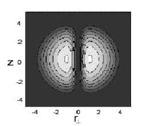
FIG. 2.: Contour plot in the $xz$ plane for a condensate with $10^{4}$ ⁸⁷Rb atoms containing a vortex along the $z$ axis. The trap is spherical and distances are in units of the oscillator length $d=0.791\ \mu$m. The interaction parameter is $Na/d=72.3$. Luminosity is proportional to density, the white area being the most dense.

(Taken from Ref. [31]).

In general, the density for a central vortex vanishes along the symmetry axis, and the core radius increases away from the center of the trap, yielding a toroidal condensate density (see Fig. 2). This behavior is particularly evident for a vortex in the TF limit $Na/d_{0}\gg 1$, when

$$n(r_{\perp},z)\approx n(0)\left(1-\frac{\xi^{2}}{r_{\perp}^{2}}-\frac{r_{\perp}^{2}}{R_{\perp}^{2}}-\frac{z^{2}}{R_{z}^{2}}\right)\Theta\left(1-\frac{\xi^{2}}{r_{\perp}^{2}}-\frac{r_{\perp}^{2}}{R_{\perp}^{2}}-\frac{z^{2}}{R_{z}^{2}}\right).$$ (37)

Here, the density differs from Eq. (28) for an axisymmetric vortex-free TF condensate only because of the dimensionless centrifugal barrier $\xi^{2}/r_{\perp}^{2}$. This term forces the density to vanish within a core whose characteristic radius is $\xi$ in the equatorial region $|z|\ll R_{z}$ and then flares out with increasing $|z|$. The TF separation of length scales ensures that the vortex affects the density only the immediate vicinity of the core [47, 62, 63]; this behavior can usually be approximated with a short-distance cutoff. For such a quantized TF vortex, the chemical potential $\mu_{1}$ differs from $\mu_{0}$ for a vortex-free TF condensate by small fractional corrections of order $(d_{0}/R_{0})^{4}\ln\,(R_{0}/d_{0})$.

2 Nonaxisymmetric trap

If a singly quantized vortex is oriented along the $z$ axis of a nonaxisymmetric trap ($R_{x}\neq R_{y}$) the condensate wave function is no longer an eigenfunction of the angular momentum operator $L_{z}$. In the TF limit near the trap center the phase $S$ of the condensate wave function has the form [64]:

$$S\approx\phi-\frac{1}{4}\left(\frac{1}{R_{x}^{2}}-\frac{1}{R_{y}^{2}}\right)r_{\perp}^{2}\ln\left(\frac{r_{\perp}}{R_{\perp}}\right)\sin(2\phi),$$ (38)

and the condensate velocity is

$${\bf v}\approx\frac{\hbar}{M}\left\{\frac{\hat{\phi}}{r_{\perp}}-\frac{1}{2}\left(\frac{1}{R_{x}^{2}}-\frac{1}{R_{y}^{2}}\right)r_{\perp}\ln\left(\frac{r_{\perp}}{R_{\perp}}\right)\left[\cos(2\phi)\hat{\phi}+\sin(2\phi)\hat{r}_{\perp}\right]\right\},$$ (39)

where $R_{\perp}^{2}=2R_{x}^{2}R_{y}^{2}/(R_{x}^{2}+R_{y}^{2})$. Near the vortex core the condensate wave function and the condensate velocity possess cylindrical symmetry, while far from the vortex core the condensate velocity adjusts to the anisotropy of the trap and becomes asymmetric.

B Thermodynamic Critical Angular Velocity for Vortex Stability

If the condensate is in rotational equilibrium at an angular velocity $\Omega$ around the $\hat{z}$ axis, the integrand of the GP Hamiltonian (6) acquires an additional term $-\Psi^{*}\Omega L_{z}\Psi$ [65], where $L_{z}=xp_{y}-yp_{x}=-i\hbar\left(x\partial_{y}-y\partial_{x}\right)$ is the $z$ component of the angular-momentum operator. Thus the Hamiltonian $H^{\prime}$ in the rotating frame becomes

$$H^{\prime}=H-\Omega L_{z}=\int dV\left[\Psi^{*}\left(T+V_{{\rm tr}}-\Omega L_{z}\right)\Psi+\frac{1}{2}g|\Psi|^{4}\right],$$ (40)

where the variables in the integrand are now those in the rotating frame. Similarly, the GP equations (4) and (5) acquire an additional term $-\Omega L_{z}\Psi$.

1 Axisymmetric trap

The situation is especially simple for an axisymmetric trap, where the states can be labeled by the eigenvalues of $L_{z}$. For example, the energy of a vortex-free condensate $E_{0}^{\prime}(\Omega)$ in the rotating frame is numerically equal to the energy $E_{0}$ in the laboratory frame because the corresponding angular momentum vanishes. A singly quantized vortex along the trap axis has the total angular momentum $N\hbar$, so that the corresponding energy of the system in the rotating frame is $E_{1}^{\prime}(\Omega)=E_{1}-N\hbar\Omega$. The difference between these two energies is the increased energy

$$\Delta E^{\prime}(\Omega)=E_{1}^{\prime}(\Omega)-E_{0}^{\prime}(\Omega)=E_{1}-E_{0}-N\hbar\Omega$$ (41)

associated with the formation of the vortex at an angular velocity $\Omega$. In the laboratory frame ($\Omega=0$), it is clear that $E_{1}>E_{0}$ because of the added kinetic energy of the circulating flow. If the condensate is in equilibrium in the rotating frame, however, $E_{1}^{\prime}(\Omega)$ decreases linearly with increasing $\Omega$, and the relative energy of the vortex vanishes at a “thermodynamic” critical angular velocity $\Omega_{c}$ determined by $\Delta E^{\prime}(\Omega_{c})=0$. Equation (41) immediately yields

$$\Omega_{c}=\frac{E_{1}-E_{0}}{N\hbar},$$ (42)

expressed solely in terms of energy of a condensate with and without the vortex evaluated in the laboratory frame.

For a noninteracting trapped gas, the difference $E_{1}-E_{0}=N\hbar\omega_{\perp}$ follows immediately from the excitation energy for the singly quantized vortex in Eq. (36) relative to the stationary ground state. In this noninteracting case, Eq. (42) gives $\Omega_{c}=\omega_{\perp}$, so that the noninteracting thermodynamic critical angular velocity is just the radial trap frequency. Indeed, the same critical angular velocity value also applies to a $q$-fold vortex in a noninteracting condensate, because of the special form of the noninteracting excitation energy $E_{q}-E_{0}=Nq\hbar\omega_{\perp}$ and the corresponding angular momentum $Nq\hbar$. Thus the noninteracting condensate becomes massively degenerate as $\Omega\to\omega_{\perp}$[66, 67]. Physically, this degeneracy reflects the cancellation between the centrifugal potential $-\frac{1}{2}M\Omega^{2}r_{\perp}^{2}$ and the radial trap potential $\frac{1}{2}M\omega_{\perp}^{2}r_{\perp}^{2}$ as $\Omega\to\omega_{\perp}$.

Numerical analysis [47] for small and medium values of $Na/d_{0}$ shows that $\Omega_{c}/\omega_{\perp}$ decreases with increasing $N$, and a perturbation analysis [67, 68] confirms this behavior for a weakly interacting system, with the analytical result $\Omega_{c}/\omega_{\perp}\approx 1-1/(2\sqrt{2\pi})\,(Na/d_{z})$ for small values of the interaction parameter $Na/d_{z}$. Figure 3 shows the behavior of $\Omega_{c}(N)$ in a spherical trap, based on numerical analysis of the GP equation with parameters relevant for ⁸⁷Rb [47].

FIG. 3.: Thermodynamic critical angular velocity $\Omega_{c}$ for the formation of a singly quantized vortex in a spherical trap with $d_{0}=0.791\ \mu$m and $N$ atoms of ⁸⁷Rb.

(Taken from Ref. [31]).

In the strongly interacting (TF) limit, the chemical potential $\mu_{1}(N)$ for a condensate containing a singly quantized vortex can be evaluated with Eq. (37), and the thermodynamic identity $\mu_{1}=\partial E_{1}/\partial N$ then yields $E_{1}(N)$. Use of the corresponding expressions for the vortex-free condensate gives the approximate expression [62, 69, 70]

$$\Omega_{c}\approx\frac{5}{2}\,\frac{\hbar^{2}}{MR_{\perp}^{2}}\ln\left(\frac{0.67R_{\perp}}{\xi}\right)\>\>\hbox{for a TF condensate}.$$ (43)

This expression exceeds the usual estimate [14] $\Omega_{c}\approx(\hbar/MR_{\perp}^{2})\ln(1.46R_{\perp}/\xi)$ for uniform superfluid in a rotating cylinder of radius $R_{\perp}$ because the nonuniform density in the trapped gas reduces the total angular momentum relative to that for a uniform fluid. Equation (43) has the equivalent form

$$\frac{\Omega_{c}}{\omega_{\perp}}\approx\frac{5}{2}\,\frac{d_{\perp}^{2}}{R_{\perp}^{2}}\ln\left(\frac{0.67R_{\perp}}{\xi}\right).$$ (44)

This ratio is small in the TF limit, because $d_{\perp}^{2}/R_{\perp}^{2}\sim\xi/R_{\perp}\ll 1$. For an axisymmetric condensate with axial asymmetry $\lambda\equiv\omega_{z}/\omega_{\perp}$, the TF relation $d_{\perp}^{2}/R_{\perp}^{2}=(d_{\perp}/15Na\lambda)^{2/5}$ shows how this ratio scales with $N$ and $\lambda$.

In contrast to the case for repulsive interactions, the thermodynamic critical angular velocity $\Omega_{c}$ for the vortex state with attractive interactions increases as the number of atoms grows [71, 47]. Since $\Omega_{c}=\omega_{\perp}$ for a noninteracting condensate, $\Omega_{c}$ for a vortex in a condensate with attractive interactions necessarily exceeds $\omega_{\perp}$. The stability or metastability of such a vortex is unclear because $\Omega=\omega_{\perp}$ is also the limit of mechanical stability for a noninteracting condensate.

Approximately the same functional relationship holds between the thermodynamic critical frequency $\Omega_{c}$ and the number of atoms in the condensate $N_{0}$ [72] for nonzero temperatures. A new feature, however, is that the number of atoms in the condensate becomes temperature-dependent:

$$\frac{N_{0}}{N}=1-\left(\frac{T}{T_{c}}\right)^{3},$$ (45)

where $T_{c}$ is the critical temperature of Bose condensation. If the trap rotates at an angular velocity $\Omega$, the distribution function of the thermal atoms changes due to the centrifugal force. As a result the critical temperature decreases according to [72]

$$\frac{T_{c}(\Omega)}{T_{c}^{0}}=\left(1-\frac{\Omega^{2}}{\omega_{\perp}^{2}}\right)^{1/3},$$ (46)

where $T_{c}^{0}$ is the critical temperature in the absence of rotation. Equations (44)-(46) allows one to calculate the critical temperature $T_{v}(\Omega)$, below which the vortex corresponds to a stable configuration in a trap rotating with frequency $\Omega$. In Fig. 4 we show the critical curves $T_{c}(\Omega)$ and $T_{v}(\Omega)$. For temperatures below $T_{c}(\Omega)$ the gas exhibits Bose-Einstein condensation. Only for temperatures below $T_{v}(\Omega)$ does the vortex state become thermodynamically stable. From Fig. 4 one can see that the critical temperature for the creation of stable vortices exhibits a maximum as a function of $\Omega$.

FIG. 4.: Phase diagram for vortices in a harmonically trapped Bose gas, $N=10^{4}$, $a/d_{\perp}=7.36\times 10^{-3}$ and $\lambda=1$.

(Taken from Ref. [72]).

2 Nonaxisymmetric trap

A rotating nonaxisymmetric trap introduces significant new physics, because the moving walls induce an irrotational flow velocity even in the absence of a vortex [49, 73, 74, 75, 76]. In the simplest case of a classical uniform fluid in a rotating elliptical cylinder, the instantaneous induced velocity potential in the laboratory frame is [49, 73]

$$\Phi_{{\rm cl}}=\Omega\,xy\,\frac{A^{2}-B^{2}}{A^{2}+B^{2}},$$ (47)

where $A$ and $B$ are the semi-axes of the elliptical cylinder. The induced angular momentum and kinetic energy are reduced from the usual solid-body values by the factor $I_{0}/I_{{\rm sb}}=\left[(A^{2}-B^{2})/(A^{2}+B^{2})\right]^{2}$. In the extreme case $B\ll A$, the moment of inertia can approach the solid-body value, even though the flow is everywhere irrotational.

The thermodynamic critical angular velocity $\Omega_{c}$ for vortex creation in the same uniform classical fluid depends on the asymmetry ratio $B/A$ [74], and experiments on superfluid ⁴He confirm the theoretical predictions in considerable detail [77]. In the limit $B\ll A$, a detailed calculation shows that $\Omega_{c}\approx(\hbar/2MB^{2})\,\ln(B/\xi)$; the appearance of $B$ here is readily understood from Feynman’s picture of a vortex occupying an area $\approx h/2M\Omega$ [compare Eq. (34)] and hence having to fit the area $\pi B^{2}$ fixed by the smaller lateral dimension $B$.

The preceding analysis for an axisymmetric dilute trapped Bose gas can be generalized to treat the TF limit in a totally anisotropic disk-shape harmonic trap with $\omega_{x}^{2}+\omega_{y}^{2}\ll\omega_{z}^{2}$, starting from Eq. (40) for the Hamiltonian in the rotating frame [78]. The presence of a vortex leaves the TF condensate density essentially unchanged, and this Hamiltonian can serve as an energy functional to determine the phase $S$ and hence the superfluid motion of the condensate. Since $R_{x}$, $R_{y}\gg R_{z}$, the curvature of the vortex is negligible. Hence we consider a singly quantized straight vortex displaced laterally from the center of the rotating trap to a transverse position ${\bf r}_{0}=(x_{0},y_{0})$ that serves as a new origin of coordinates. The condensate wave function then has the form

$$\Psi=|\Psi|\,e^{i\phi+iS_{0}},$$ (48)

where $\phi$ in the first term is the polar angle around the vortex axis and $S_{0}$ is a periodic function of $\phi$. Varying the Hamiltonian gives an Euler-Lagrange equation for $S_{0}$, and it can be well approximated by the solution for a vortex-free condensate, which is $M/\hbar$ times the classical expression (47) with $A$ and $B$ replaced by the TF radii $R_{x}$ and $R_{y}$ given in Eq. (29), and with $x$ and $y$ shifted to the new origin.

As in Eq. (41) for an axisymmetric trap, $\Delta E^{\prime}(x_{0},y_{0},\Omega)$ gives the increased energy in the rotating frame associated with the presence of the straight vortex. A detailed calculation with logarithmic accuracy yields [78]

$$\Delta E^{\prime}(x_{0},y_{0},\Omega)=\frac{8\pi}{3}\mu R_{z}\,\xi^{2}n(0)\left(1-\zeta_{0}^{2}\right)^{3/2}\left[\ln\left(\frac{R_{\perp}}{\xi}\right)-\frac{8}{5}\,\frac{\mu\Omega}{\hbar\left(\omega_{x}^{2}+\omega_{y}^{2}\right)}\left(1-\zeta_{0}^{2}\right)\right],$$ (49)

where $\zeta_{0}^{2}\equiv x_{0}^{2}/R_{x}^{2}+y_{0}^{2}/R_{y}^{2}\leq 1$ is a dimensionless displacement of the vortex from the trap center. Here, the mean transverse condensate radius $R_{\perp}$ is given by the arithmetic mean of the inverse squared radii

$$\frac{1}{R_{\perp}^{2}}=\frac{1}{2}\left(\frac{1}{R_{x}^{2}}+\frac{1}{R_{y}^{2}}\right)=\frac{M\left(\omega_{x}^{2}+\omega_{y}^{2}\right)}{4\mu}.$$ (50)

Figure 5 shows the behavior of $\Delta E^{\prime}(\zeta_{0},\Omega)$ as a function of $\zeta_{0}$ for various fixed values of $\Omega$. Curve (a) for $\Omega=0$ shows that the corresponding energy $\Delta E^{\prime}(\zeta_{0},\Omega=0)$ decreases monotonically with increasing $\zeta_{0}$, with negative curvature at $\zeta_{0}=0$. In the absence of dissipation, energy is conserved and the vortex follows an elliptical trajectory at fixed $\zeta_{0}$ around the center of the trap along a line $V_{{\rm tr}}={\rm const}$. At low but finite temperature, however, the vortex experiences weak dissipation; thus it slowly reduces its energy by moving outward along curve (a), executing a spiral trajectory in the $xy$ plane.

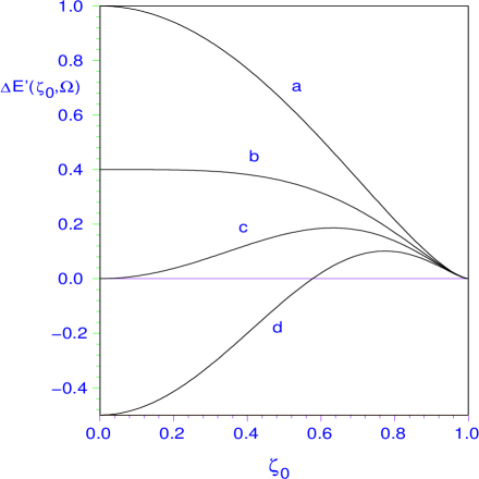
FIG. 5.: Energy (49) [in units of $\Delta E^{\prime}(0,0)$] associated with a singly quantized straight vortex in a rotating asymmetric trap in the TF limit as a function of a fractional vortex displacement $\zeta_{0}$ from the symmetry axis. Different curves represent different fixed values of the external angular velocity $\Omega$: (a) $\Omega=0$ (unstable); (b) $\Omega=\Omega_{m}$ [given in Eq. (51)] (onset of metastability at the origin); (c) $\Omega=\Omega_{c}$ [given in Eq. (52)] (onset of stability at origin); (d) $\Omega=\frac{3}{2}\Omega_{c}$, where the thin barrier hinders vortex tunneling from the surface.

With increasing fixed rotation speed $\Omega$, the function $\Delta E^{\prime}(\zeta_{0},\Omega)$ flattens. Curve (b) shows the special case of zero curvature at $\zeta_{0}=0$. It corresponds to the rotation speed

$$\Omega_{m}=\frac{3}{2}\frac{\hbar}{MR_{\perp}^{2}}\ln\left(\frac{R_{\perp}}{\xi}\right)\quad\hbox{for a disk-shape condensate},$$ (51)

at which angular velocity a central vortex first becomes metastable in a large disk-shape condensate. For $\Omega<\Omega_{m}$, the negative local curvature at $\zeta_{0}=0$ means that weak dissipation impels the vortex away from the center. For $\Omega>\Omega_{m}$, however, the positive local curvature means that weak dissipation now impels the vortex back toward the center of the trap. In this regime, the central position is locally stable; it is not globally stable, however, because $\Delta E^{\prime}(0,\Omega)$ is positive for $\Omega\approx\Omega_{m}$.

Curve (c) shows that $\Delta E^{\prime}(0,\Omega_{c})$ vanishes at the thermodynamic critical angular velocity

$$\Omega_{c}=\frac{5}{2}\frac{\hbar}{MR_{\perp}^{2}}\ln\left(\frac{R_{\perp}}{\xi}\right)=\frac{5}{3}\Omega_{m}\quad\hbox{for a disk-shape condensate}.$$ (52)

As expected, this expression (52) reduces to Eq. (43) in the limit of an axisymmetric disk-shape condensate. For $\Omega>\Omega_{c}$, the central vortex is both locally and globally stable relative to the vortex-free state, and the energy barrier near the outer surface of the condensate becomes progressively narrower. Curve (d) illustrates this behavior for $\Omega=\frac{3}{2}\Omega_{c}$. Eventually, the barrier thickness becomes comparable with the thickness of the boundary layer within which the TF approximation fails[79], and it has been suggested that a vortex might then nucleate spontaneously through a surface instability [80, 76, 81]. For a two-dimensional condensate, a phase diagram for different critical velocities of trap rotation vs. the system parameter $an_{z}$ ($n_{z}$ is the area density) is given in [81].

C Experimental Creation of a single vortex

The first experimental detection of a vortex involved a nearly spherical ⁸⁷Rb TF condensate containing two different internal (hyperfine) components [33] that tend to separate into immiscible phases. The JILA group in Boulder created the vortex through a somewhat intricate coherent process that controlled the interconversion between the two components (discussed below in Sec. VII). In essence, the coupled two-component system acts like an $SU(2)$ spin-$\frac{1}{2}$ system whose topology differs from the usual $U(1)$ complex one-component order parameter $\Psi$ familiar from superfluid ⁴He (and conventional BCS superconductivity). Apart from the magnitude $|\Psi|$ that is fixed by the temperature in a uniform system, a one-component order parameter has only the phase that varies between 0 and $2\pi$. This topology is that of a circle and yields quantized vorticity to ensure that the order parameter is single-valued [10, 11]. In contrast, a two-component system has two degrees of freedom in addition to the overall magnitude; its topology is that of a sphere and does not require quantized vorticity. The qualitative difference between the two cases can be understood as follows: the single degree of freedom of the one-component order parameter is like a rubber band wrapped around a cylinder, while the corresponding two degrees of freedom for the two-component order parameter is like a rubber band around the equator of a sphere. The former has a given winding number that can be removed only be cutting it (ensuring the quantization of circulation), whereas the latter can be removed simply by pulling it to one of the poles (so that there is no quantization).

The JILA group was able to spin up the condensate by coupling the two components. They then turned off the coupling, leaving the system with a residual trapped quantized vortex consisting of one circulating component surrounding a nonrotating core of the other component, whose size is determined by the relative fraction of the two components. By selective tuning, they can image either component nondestructively [37]; Fig. 6 shows the precession of the filled vortex core around the trap center. In addition, an interference procedure allowed them to map the variation of the cosine of the phase around the vortex, clearly showing the expected sinusoidal variation (Fig. 7).

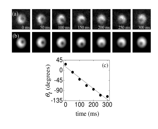
FIG. 6.: (a) Successive images of a condensate with a vortex. The recorded profile of each trapped condensate is fit with a smooth TF distribution (b). The vortex core is the dark region within the bright condensate image. (c) The azimuthal angle of the core is determined for each image, and plotted vs. time held in the trap. A linear fit to the data gives a precession frequency 1.3(1) Hz.

(Taken from Ref. [37]).

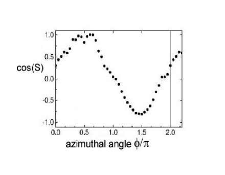
FIG. 7.: Cosine of the phase around the vortex, showing the sinusoidal variation expected for the azimuthal angle.

(Taken from Ref. [33]).

The JILA group has also been able to remove the component filling the core, in which case they obtain a single-component vortex [37]. This one-component vortex has a small core size and can only be imaged by expanding both the condensate and the core, which becomes visible through its reduced density [82, 70]. They first make an image of the two-component vortex, next remove the component filling the core, and then make an image of the one-component vortex after a variable time delay. In this way, they can measure the precession rate of the one-component empty-core vortex and compare it with theoretical predictions [83]. The data show no tendency for the core to spiral outward, suggesting that the thermal damping is negligible on the time scale of $\sim 1$ s.

Separately, the ENS group in Paris observed the formation of one and more vortices in a single-component ⁸⁷Rb elongated cigar-shape TF condensate with a weak nonaxisymmetric deformation that rotates about its long axis [34, 35, 36]. In essence, a static cylindrically symmetric magnetic trap is augmented by a nonaxisymmetric attractive dipole potential created by a stirring laser beam. The combined potential produces a cigar-shape harmonic trap with a slightly anisotropic transverse profile. The transverse anisotropy rotates slowly at a rate $\Omega\lesssim 200$ Hz. In the first experiments [34], the trap was rotated in the normal state and then cooled, with the clear signal of the vortex shown in Fig. 8 (the trap was turned off, allowing the atomic cloud to expand so that the vortex core becomes visible). This order was reversed (cool first, then rotate) in a later series of runs [36]. In both cases, the observed critical angular velocity $\sim 0.7\omega_{\perp}$ for creating the first (central) vortex was roughly 70% higher than the predicted thermodynamic value $\Omega_{c}$ in Eq. (43). These observations agree qualitatively with the suggestion that a surface instability might nucleate a vortex [80, 76, 81]. Alternative explanations of this discrepancy involve the bending modes of the vortex (discussed below in Sec. IV.D.4 and V.D.2).

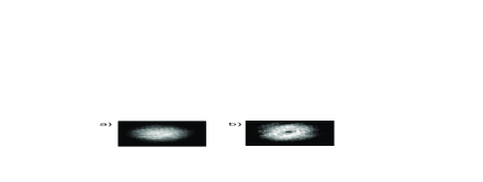
FIG. 8.: Optical thickness of the expanded clouds in the transverse direction showing the difference between the states (a) without and (b) with a vortex.

(Taken from Ref. [34]).

D Vortex Arrays

Under appropriate stabilization conditions, such as steady applied rotation, vortices can form a regular array. In a rotating uniform superfluid, the quantized vortex lines parallel to the axis of rotation form a lattice. This lattice rotates as a whole around the axis of rotation, thus simulating rigid rotation [84]. At nonzero temperature, dissipative mutual friction from the normal component ensures that the array rotates with the same angular velocity as the container. Early experiments on rotating superfluid ⁴He [85, 13, 86] provided memorable “photographs” of vortex lines and arrays with relatively small numbers of vortices, in qualitative agreement with analytical [87, 88] and numerical [89, 90] predictions. A triangular array is favored for vortices near the rotation axis of rapidly rotating vessels of superfluid helium [87]. Vortex lattices also occur in the neutron superfluid in rotating neutron stars [16].

Even before the recent observation of vortex arrays in an elongated rotating trapped condensate [34, 35], several theoretical groups had analyzed many of the expected properties. In a weakly interacting (near-ideal) axisymmetric condensate, the thermodynamic critical angular velocity $\Omega_{c}$ for the appearance of the first vortex is already close to the radial trap frequency $\omega_{\perp}$, so that the creation of additional vortices involves many states $\phi_{m}({\bf r}_{\perp})\propto e^{im\phi}\,r_{\perp}^{m}\,\exp(-\frac{1}{2}r_{\perp}^{2}/d_{\perp}^{2})$ with low energy $m\hbar(\omega_{\perp}-\Omega)$ per particle in the rotating frame. Butts and Rokhsar [67] used a linear combination of these nearly degenerate states as a variational condensate wave function, minimizing the total energy in the laboratory frame $E_{{\rm lab}}$ subject to the condition of fixed number $N$ of particles and fixed angular momentum $l$ per particle. As expected from the theoretical and experimental results for liquid helium, the system undergoes a sequence of transitions between states that break rotational symmetry. Several of these have $p$-fold symmetry where $p$ is a small integer. Each vortex represents a node in the condensate wave function, and their positions can vary with the specified angular momentum. Indeed, as $l$ increases from 0 to 1, the first vortex moves continuously from the edge of the condensate to the center. For larger number of vortices, the centrifugal forces tend to flatten and expand the condensate in the radial direction. In this approach of keeping $l$ fixed, the angular velocity follows from the relation $\hbar\Omega=\partial E_{{\rm lab}}/\partial l$. Figure 9 shows the angular momentum versus the angular velocity for the first several states. Reference [91] has carried out more detailed studies of the states for relatively small values of the angular momentum per particle $l\lesssim 2$.

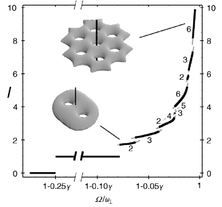
FIG. 9.: Dimensionless angular momentum $l$ per particle vs. dimensionless angular velocity $\Omega/\omega_{\perp}$. In the figure $\gamma=(2/\pi)^{1/2}aN/d_{z}$. Black lines show stable states and gray lines show metastable states. There are no stable or metastable states in the forbidden ranges $l=0$-1 and $l=1$-1.70. The rotational symmetry of each branch is indicated. The total angular momentum diverges as $\Omega$ approaches the maximum angular velocity $\omega_{\perp}$. Three-dimensional plots of constant density show states with two-fold and six-fold symmetry. Reprinted by permission from Nature 397, 327, (1999), ©1999 Macmillan Magazines Ltd.

These analyses work at fixed angular momentum $Nl$, in which case the angular velocity $\Omega$ must be determined from the resulting $E_{{\rm lab}}(l)$. In contrast, the ENS experiments fix $\Omega$ (as do experiments on superfluid helium) and then measure $L_{z}$ from the splitting of the quadrupole modes [36] (see Sec. IV.D.3). The JILA group [92] also uses this technique to detect the presence of a vortex in a nonrotating condensate. The transition from fixed $L_{z}$ to fixed $\Omega$ can be considered a Legendre transformation to the Hamiltonian (40) in the rotating frame. Even though it is easier to work at fixed $\Omega$ (because there is no constraint of fixed $L_{z}/N=l$), no such analysis has yet been carried out in the weak-coupling limit.

In the strong-coupling (TF) limit, Castin and Dum [70] have performed extensive numerical studies of equilibrium vortex arrays in two and three dimensions, based on the Hamiltonian in the rotating frame (thus working at fixed $\Omega$). They also propose an intuitive variational calculation based on a factorization approximation that is very similar to Eq. (26), apart from a different analytic form of the radial function [52, 53].

The nucleation of vortices and the resulting structures of vortex arrays in zero temperature BECs are also investigated numerically by Feder, Clark and Schneider [76]. In their simulations, vortices are generated by rotating a three-dimensional, nonaxisymmetric harmonic trap. Vortices first appear at a rotation frequency significantly larger than the critical frequency for vortex stabilization. At higher frequencies, the trap geometry strongly influences the structure of the vortex arrays, but the lattices approach triangular arrays at large vortex densities.

The ENS experiments [34, 35] have produced remarkable images of vortex arrays. Figure 10 shows three different arrays with up to 11 vortices (obtained after an expansion of 27 ms). The initial condensate is very elongated (along with the vortices), so that the radial expansion predominates once the trap is turned off. As a result, the expanded condensate acquires a pancake shape similar to that in Fig. 9.

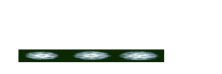
FIG. 10.: Arrays of vortices in a Bose-Einstein condensate stirred with a laser beam.

(Taken from Ref. [35]).

IV Bogoliubov equations: stability of small-amplitude perturbations

This section considers only the behavior of a dilute one-component Bose gas, for which the analysis of the eigenfrequencies is particularly direct. In the more general case of two interpenetrating species, even a uniform system can have imaginary frequencies for sufficiently strong interspecies repulsion [93, 94]; this dynamical instability signals the onset of phase separation.

A General features for nonuniform condensate

The special character of an elementary excitation in a dilute Bose gas largely arises from the role of the Bose condensate that acts as a particle reservoir. This situation is especially familiar in the uniform system, where an elementary excitation with wave vector ${\bf k}$ can arise from the interacting ground state $\Psi_{0}$ either through the creation operator $a_{{\bf k}}^{\dagger}$ or through the annihilation operator $a_{-{\bf k}}$ (in the thermodynamic limit, these two states $a_{{\bf k}}^{\dagger}\Psi_{0}$ and $a_{-{\bf k}}\Psi_{0}$ differ only by a normalization factor). The true excited eigenstates are linear combinations of the two states, and the corresponding operator for the Bogoliubov quasiparticle is a weighted linear combination [38, 42, 43]

$$\alpha_{{\bf k}}^{\dagger}=u_{k}\,a_{{\bf k}}^{\dagger}+v_{k}\,a_{-{\bf k}},$$ (53)

where $u_{k}$ and $v_{k}$ are the (real) Bogoliubov coherence factors. This linear transformation (53) is canonical if the quasiparticle operators also obey Bose-Einstein commutation relations, which readily yields the condition

$$u_{k}^{2}-v_{k}^{2}=1,\quad\hbox{for all ${\bf k}\neq 0$}.$$ (54)

More generally, the second-quantized Bose field operator $\hat{\psi}$ in Eq. (2) can be written as $\hat{\psi}({\bf r})\approx\Psi({\bf r})+\hat{\phi}({\bf r})$, where $\hat{\phi}$ is a small deviation operator from the macroscopic condensate wave function $\Psi$. These deviation operators obey the approximate Bose-Einstein commutation relations

$$\left[\hat{\phi}({\bf r}),\hat{\phi}^{\dagger}({\bf r}^{\prime})\right]\approx\delta\!\left({\bf r-r}^{\prime}\right),\quad\left[\hat{\phi}({\bf r}),\hat{\phi}({\bf r}^{\prime})\right]=\left[\hat{\phi}^{\dagger}({\bf r}),\hat{\phi}^{\dagger}({\bf r}^{\prime})\right]\approx 0.$$ (55)

Since $\hat{\psi}({\bf r})$ does not conserve particle number, it is convenient to use a grand canonical ensemble, with the new Hamiltonian operator $\hat{K}=\hat{H}-\mu\hat{N}$ instead of the Hamiltonian (1). To leading (second) order in the small deviations, the perturbation in $\hat{K}$ contains not only the usual “diagonal” terms involving $\hat{\phi}^{\dagger}\hat{\phi}$, but also “off-diagonal” terms proportional to $\hat{\phi}\hat{\phi}$ and $\hat{\phi}^{\dagger}\hat{\phi}^{\dagger}$. Consequently, the resulting Heisenberg operators $\hat{\phi}$ and $\hat{\phi}^{\dagger}$ obey coupled linear equations of motion (it is here that the role of the condensate is evident, for this coupling vanishes if $\Psi$ vanishes). Pitaevskii [41] developed this approach for the particular case of a vortex line in unbounded condensate, and the formalism was subsequently extended to include a general nonuniform condensate [95, 96].

In direct analogy to the Bogoliubov transformation for the uniform system, assume the existence of a linear transformation to quasiparticle operators $\alpha_{j}$ and $\alpha_{j}^{\dagger}$ for a set of normal modes labeled by $j$

$$\hat{\phi}({\bf r},t)={\sum_{j}}^{\prime}\left[u_{j}({\bf r})\alpha_{j}(t)-v_{j}^{*}({\bf r})\alpha_{j}^{\dagger}(t)\right],$$ (57)

$$\hat{\phi}^{\dagger}({\bf r},t)={\sum_{j}}^{\prime}\left[u_{j}^{*}({\bf r})\alpha_{j}^{\dagger}(t)-v_{j}({\bf r})\alpha_{j}(t)\right],$$ (58)

where the primed sum means to omit the condensate mode. Here, the quasiparticle operators $\alpha_{j}$ and $\alpha_{k}^{\dagger}$ obey Bose-Einstein commutation relations $\left[\alpha_{j},\alpha_{k}^{\dagger}\right]=\delta_{jk}$ and have simple harmonic time dependences $\alpha_{j}(t)=\alpha_{j}\,\exp\left(-iE_{j}t/\hbar\right)$ and $\alpha_{j}^{\dagger}(t)=\alpha_{j}^{\dagger}\,\exp\left(iE_{j}t/\hbar\right)$. Comparison with the equations of motion for $\hat{\phi}$ and $\hat{\phi}^{\dagger}$ shows that the corresponding spatial amplitudes obey a set of coupled linear “Bogoliubov equations”

$$Lu_{j}-g\left(\Psi\right)^{2}v_{j}=E_{j}u_{j},$$ (60)

$$Lv_{j}-g\left(\Psi^{*}\right)^{2}u_{j}=-E_{j}v_{j},$$ (61)

where

$$L=T+V_{{\rm tr}}-\mu+2g|\Psi|^{2}$$ (62)

is a Hermitian operator.

Straightforward manipulations with the Bogoliubov equations show that $E_{j}\int dV\left(|u_{j}|^{2}-|v_{j}|^{2}\right)$ is real. If the integral $\int dV\left(|u_{j}|^{2}-|v_{j}|^{2}\right)$ is nonzero, then $E_{j}$ itself is real. Like Eq. (54) for a uniform condensate, the Bose-Einstein commutation relations (55) for the deviations from the nonuniform condensate can be shown to imply the following positive normalization [95]

$$\int dV\left(|u_{j}|^{2}-|v_{j}|^{2}\right)=1.$$ (63)

For each solution $u_{j},v_{j}$ with eigenvalue $E_{j}$ and positive normalization, the Bogoliubov equations always have a second solution $v_{j}^{*},u_{j}^{*}$ with eigenvalue $-E_{j}$ and negative normalization. The only exception to the requirement of real eigenvalues arises for zero-norm solutions with $\int dV\left(|u_{j}|^{2}-|v_{j}|^{2}\right)=0$. In this case the character of the eigenvalue requires additional analysis. Numerical investigations [97] of vortices in nonuniform trapped condensates have reported imaginary and/or complex eigenfrequencies for doubly quantized vortices but only real eigenfrequencies for singly quantized vortices. Specifically, for a repulsive interparticle interaction, Pu et al. [97] found that singly quantized vortices are always intrinsically stable; in contrast, multiply quantized vortices have alternating stable and unstable regions with complex excitation energy as the interaction parameter $Na/d$ increases. The most unstable vortex state decays after several periods of the harmonic trapping potential. In the case of multiply quantized vortices ($q>1$), the vortex core contains localized quasiparticle bound states with small exponential tails; these modes have complex frequencies and are responsible for splitting the multicharged core [98]. For an attractive interaction, stable vortices exist only for the singly quantized case in the weak-interaction regime; a multiply quantized vortex state is always unstable. Similar imaginary and complex solutions have been found for dark solitons [99, 100, 101]. For additional results on complex eigenfrequencies, see Ref. [102] and the Appendix of Ref. [103].

In terms of the quasiparticle operators, the approximate perturbation Hamiltonian operator takes the simple intuitive form

$$\hat{K}^{\prime}\approx{\sum_{j}}^{\prime}\,E_{j}\,\alpha_{j}^{\dagger}\alpha_{j},$$ (64)

apart from a constant ground-state contribution of all the normal modes. Here, the sum is over all the states with positive normalization, and it is clear that the sign of the energy eigenvalues $E_{j}$ is crucial for the stability. If one or more of the eigenvalues is negative, the Hamiltonian is no longer positive definite, and the system can lower its energy by creating quasiparticles in the unstable modes.

The present derivation of the Bogoliubov equations and their properties emphasizes the quantum-mechanical basis for the positive normalization condition (63) and the sign of the eigenvalues. It is worth noting an alternative purely “classical” treatment [104, 31] based directly on small perturbations of the time-dependent GP equation (4) around the static condensate $\Psi({\bf r})$. The solution is assumed to have the form

$$\Psi({\bf r},t)=e^{-i\mu t/\hbar}\left[\Psi({\bf r})+u({\bf r})e^{-i\omega t}-v^{*}({\bf r})e^{i\omega t}\right],$$ (65)

and the appropriate eigenvalue equations then reproduce Eqs. (IV A).

B Uniform condensate

For a uniform condensate, the solutions of Eq. (IV A) are plane waves, and the corresponding energy is the celebrated Bogoliubov spectrum [38]

$$E_{k}=\sqrt{gn\hbar^{2}k^{2}/M+\left(\hbar^{2}k^{2}/2M\right)^{2}},$$ (66)

where ${\bf k}$ is the wave vector of the excitation and $n$ is the condensate density. For long wavelengths $k\xi\ll 1$, Eq. (66) reduces to a linear phonon spectrum $E_{k}\approx\hbar sk$ with the speed of compressional sound $s=\sqrt{gn/M}$ given by Eq. (10). In the opposite limit $k\xi\gg 1$, the spectrum reduces to the free-particle form plus a mean-field Hartree shift from the interaction with the background condensate $E_{k}\approx(\hbar^{2}k^{2}/2M)+gn$.

To understand the importance of the sign of the eigenfrequency, it is instructive to consider the case of a condensate that moves uniformly with velocity ${\bf v}_{0}$. As noted in connection with Eq. (24), the condensate wave function is $\Psi({\bf r})=\sqrt{n}\,e^{i{\bf q\cdot r}}$, where ${\bf q}=M{\bf v}_{0}/\hbar$ and the chemical potential becomes $\mu=\frac{1}{2}Mv_{0}^{2}+gn$. The Bogoliubov amplitudes for an excitation with wave vector ${\bf k}$ relative to the moving condensate have the form

$$\pmatrix{u_{\bf k}({\bf r})\cr v_{\bf k}({\bf r})}=\pmatrix{e^{i\bf q\cdot r}\,u_{k}e^{i\bf k\cdot r}\cr e^{-i\bf q\cdot r}\,v_{k}e^{i\bf k\cdot r}},$$ (67)

where the different signs $\pm i{\bf q\cdot r}$ arise from the different phases $\pm i2{\bf q\cdot r}$ in the off-diagonal coupling terms in the Bogoliubov equations (IV A). The solution with positive norm has the eigenvalue

$$E_{{\bf k}}({\bf v}_{0})=\hbar{\bf k\cdot v}_{0}+E_{k},$$ (68)

as expected from general considerations [105, 106]. In the long-wavelength limit, this excitation energy reduces to $E_{{\bf k}}({\bf v}_{0})\approx\hbar k(v_{0}\cos\theta+s)$, where $\theta$ is the angle between ${\bf k}$ and ${\bf v}_{0}$. For $v_{0}<s$, the quasiparticle energy is positive for all angles $\theta$, but for $v_{0}>s$, the quasiparticle energy becomes negative for certain directions, indicating the onset of an instability. This behavior simply reflects the well-known Landau critical velocity for the onset of dissipation, associated with the emission of quasiparticles. It has many analogies with supersonic flow in classical compressible fluids [107] and Cherenkov radiation of photons in a dielectric medium [108, 109]. For $v_{0}>s$, the GP description becomes incomplete because the excitation of quasiparticles means that the noncondensate is no longer negligible.

C Quantum-hydrodynamic description of small-amplitude normal modes

The quantum-hydrodynamic forms (16) and (17) of the time-dependent GP equation provide a convenient alternative basis for studying the small-amplitude normal modes. The small perturbations in the density $n^{\prime}e^{-i\omega t}$ and the velocity potential $\Phi^{\prime}e^{-i\omega t}$ obey coupled linear equations [96, 110, 111] that reduce to Eq. (33) in the TF limit for a static condensate [57]. A comparison with Eqs. (IV A) shows that the quantum-hydrodynamic amplitudes

$$n_{j}^{\prime}=\Psi^{*}\,u_{j}-\Psi\,v_{j}=|\Psi|\left(e^{-iS}u_{j}-e^{iS}v_{j}\right),$$ (70)

$$\Phi_{j}^{\prime}=\frac{\hbar}{2Mi\,|\Psi|^{2}}\left(\Psi^{*}\,u_{j}+\Psi\,v_{j}\right)=\frac{\hbar}{2Mi\,|\Psi|}\left(e^{-iS}u_{j}+e^{iS}v_{j}\right)$$ (71)

are simply linear combinations of the Bogoliubov amplitudes $u_{j}$ and $v_{j}$ in the presence of the given condensate solution $\Psi=e^{iS}|\Psi|$. The positive normalization condition (63) yields the equivalent quantum-hydrodynamic form

$$\int dV\,i\left({n_{j}^{\prime}}^{*}\Phi_{j}^{\prime}-{\Phi_{j}^{\prime}}^{*}n_{j}^{\prime}\right)=\frac{\hbar}{M}.$$ (72)

For many purposes, the quantum-hydrodynamic modes provide a clearer picture of the dynamical motion.

D Singly quantized vortex in axisymmetric trap

Early numerical studies for small and medium values of the interaction parameter $Na/d_{0}\lesssim~{}1$ examined the small-amplitude excitations of a condensate with a singly quantized vortex [112]. In particular, the spectrum contained an “anomalous” mode with a negative excitation frequency and positive normalization associated with a large Bogoliubov amplitude $u$ localized in the vortex core (see also relevant comments in Ref. [63] concerning the relationship between the sign of the normalization and the sign of the eigenfrequency). The anomalous mode corresponds to a precession of the vortex line around $z$ axis. As seen from the general discussion of the Bogoliubov equations, this anomalous mode indicates the presence of an instability.

Since the condensate wave function has an explicit phase $\Psi({\bf r})=e^{i\phi}\,|\Psi(r_{\perp},z)|$, the Bogoliubov amplitudes for an excitation with angular momentum $m\hbar$ relative to the vortex condensate take the form

$$\pmatrix{u_{m}({\bf r})\cr v_{m}({\bf r})}=\pmatrix{e^{i\phi}\,e^{im\phi}\tilde{u}_{m}(r_{\perp},z)\cr e^{-i\phi}\,e^{im\phi}\tilde{v}_{m}(r_{\perp},z)}.$$ (73)

analogous to those in Eq. (67) for a condensate in uniform motion. Here, the azimuthal quantum number $m$ characterizes the associated density and velocity deformations of the vortex proportional to $e^{im\phi}$ [for example, $n_{m}^{\prime}=|\Psi|\left(\tilde{u}_{m}-\tilde{v}_{m}\right)e^{im\phi}$, as is clear from Eqs. (IV C)]. The numerical studies [112] found that the anomalous mode has an azimuthal quantum number $m_{a}=-1$. Its frequency $\omega_{a}$ is negative throughout the relevant range of $Na/d_{0}\lesssim 1$; in the noninteracting limit, $\omega_{a}$ approaches $-\omega_{\perp}$, and $\omega_{a}$ increases toward $0$ from below with increasing $Na/d_{0}$.

To understand the particular value $m_{a}=-1$, it is helpful to recall the noninteracting limit, when the negative anomalous mode for the vortex condensate signals the instability associated with Bose condensation in the first excited harmonic-oscillator state with excitation energy $\hbar\omega_{\perp}$ and unit angular momentum. A particle in the condensate can make a transition from the vortex state back to the true harmonic-oscillator ground state, with a change in frequency $-\omega_{\perp}$ and a change in angular momentum quantum number $-1$. More generally, the density perturbation $n_{a}^{\prime}$ for the anomalous mode with negative frequency $-|\omega_{a}|$ is proportional to $\exp\left[i\left(|\omega_{a}|t-\phi\right)\right]$ and hence precesses in the positive sense (namely counterclockwise) at the frequency $|\omega_{a}|$. Thus the anomalous mode describes the JILA observations of the precession frequency of a one-component vortex [37, 83].

1 Near-ideal regime

An explicit perturbation analysis [113, 68] of the GP equation for the condensate wave function in the weakly interacting limit found the thermodynamic critical angular velocity

$$\frac{\Omega_{c}}{\omega_{\perp}}=1-\frac{1}{\sqrt{8\pi}}\frac{Na}{d_{z}}+\Omega_{c}^{(2)}(\lambda)\left(\frac{Na}{d_{z}}\right)^{\!\!2}+\cdots\ ,$$ (74)

where the second-order correction depends explicitly on the axial asymmetry $\lambda=\omega_{z}/\omega_{\perp}$. Similarly, a perturbation expansion of the Bogoliubov equations in the weak-coupling limit verified the numerical analysis and found the explicit expression for the frequency of the anomalous mode

$$\frac{\omega_{a}}{\omega_{\perp}}=-1+\frac{1}{\sqrt{8\pi}}\frac{Na}{d_{z}}+\omega_{a}^{(2)}(\lambda)\left(\frac{Na}{d_{z}}\right)^{\!\!2}+\cdots\ .$$ (75)

It is evident that $\Omega_{c}+\omega_{a}$ vanishes through first order, and the detailed analysis shows that the second-order contribution to the sum is positive for all values of the axial asymmetry parameter $\lambda$.

The physics of the anomalous mode can be clarified by considering an axisymmetric condensate in rotational equilibrium at an angular velocity $\Omega$ around the $\hat{z}$ axis. In the rotating frame, the Hamiltonian becomes $H-\Omega L_{z}$, and the Bogoliubov amplitudes have frequencies $\omega_{j}(\Omega)=\omega_{j}-m_{j}\Omega$, where $\omega_{j}$ is the frequency in the nonrotating frame and $m_{j}$ is the azimuthal quantum number [see Eq. (73)]. For the anomalous mode with $m_{a}=-1$, the resulting frequency in the rotating frame is

$$\omega_{a}(\Omega)=\omega_{a}+\Omega,$$ (76)

which is directly analogous to Eq. (68) for uniform translation. Since $\omega_{a}$ is negative, the anomalous frequency in a rotating frame increases linearly toward zero with increasing $\Omega$; in particular, $\omega_{a}(\Omega)$ vanishes at a characteristic rotation frequency

$$\Omega^{*}=-\omega_{a}=|\omega_{a}|$$ (77)

that signals the onset of the regime $\Omega\geq\Omega^{*}$ for which the singly quantized vortex becomes locally stable. Equation (75) gives an explicit expression for $\Omega^{*}$ in the weak-coupling limit, and detailed comparison with Eq. (74) indicates that $\Omega^{*}<\Omega_{c}$ for any axial asymmetry $\lambda$ (but only because of the second-order contributions). It is natural to identify $\Omega^{*}$ with the angular velocity for the onset of local stability with respect to small perturbations; this quantity was denoted $\Omega_{m}$ in connection with the equilibrium energy in the TF limit (see Fig. 5).

2 Thomas-Fermi regime for disk-shape trap

The anomalous negative-frequency mode exists only because the condensate contains a vortex. Hence it cannot be analyzed by treating the vortex itself as a perturbation. In the TF limit, however, it is possible to use Gross’s and Pitaevskii’s [39, 41] solution (19) for a vortex in a laterally unbounded fluid as the basis for a perturbation expansion. A detailed analysis of the Bogoliubov equations for an axisymmetric rotating flattened trap in the TF limit yields the explicit expression for the anomalous mode [114]

$$\omega_{a}(\Omega)=\Omega-\frac{3\hbar\omega_{\perp}^{2}}{4\mu}\ln\left(\frac{R_{\perp}}{\xi}\right)=\Omega-\frac{3}{2}\frac{\hbar}{MR_{\perp}^{2}}\ln\left(\frac{R_{\perp}}{\xi}\right).$$ (78)

As in Eq. (77) for the weak-coupling limit, Eq. (78) yields

$$\Omega^{*}=\frac{3}{2}\frac{\hbar}{MR_{\perp}^{2}}\ln\left(\frac{R_{\perp}}{\xi}\right)=\Omega_{m}=\frac{3}{5}\Omega_{c},$$ (79)

where the last two equalities follow from (51) and (52). This relation further supports the identification of $\Omega^{*}$ with the metastable rotation frequency $\Omega_{m}$ associated with local stability of a vortex for small lateral displacements from the center of the trap. Note that $\Omega_{m}<\Omega_{c}$ for a disk-shape condensate (in the TF limit) [see Eqs. (51) and (52)], similar to the behavior for the weak-coupling regime.

3 Quantum-hydrodynamic analysis of condensate normal modes in the Thomas-Fermi regime

In addition to the anomalous mode described above, the condensate has a sequence of normal modes that occur both with and without a vortex. Indeed, one of the early triumphs of the quantum-hydrodynamic description [57] was the detailed agreement between the theoretical predictions and the measured frequencies of the lowest few collective normal modes [31]. For an axisymmetric condensate, the normal modes can be classified by their azimuthal quantum number $m$, and modes with $\pm m$ are degenerate for a stationary condensate.

When the condensate contains a vortex, however, the various collective modes are perturbed. In particular, the vortex breaks time-reversal symmetry by imposing a preferred sense of rotation, so that modes with $\pm m$ are split (this behavior is analogous to the Zeeman effect in which an applied magnetic field splits the magnetic sublevels). In fact, the splitting of these degenerate hydrodynamic modes has been used to detect the presence of a vortex [36, 92] and to infer its circulation and angular momentum.

In the context of the quantum-hydrodynamic description, the principal effect of the vortex arises through its circulating velocity field ${\bf v}$, which shifts the time derivative $\partial_{t}\to\partial_{t}+\mathchoice{{\hbox{\boldmath$\displaystyle\nabla$}}}{{\hbox{\boldmath$\textstyle\nabla$}}}{{\hbox{\boldmath$\scriptstyle\nabla$}}}{{\hbox{\boldmath$\scriptscriptstyle\nabla$}}}\cdot{\bf v}$. For a normal mode $\propto e^{im\phi}$ with azimuthal quantum number $m$, the perturbation in the frequency has the form $m\hbar/Mr_{\perp}^{2}$. A detailed analysis shows that the fractional splitting of the modes is of order $(\omega_{+}-\omega_{-})/\omega_{+}\sim|m|d_{\perp}^{2}/R_{\perp}^{2}$, with a numerical coefficient that depends on the particular mode in question [62, 111]. Independently, Zambelli and Stringari [115] used sum rules to calculate the vortex-induced splitting of the lowest quadrupole mode with $m=\pm 2$; the two approaches yield precisely the same expressions. In the absence of a vortex, the $|m|=2$ mode simply involves an oscillating quadrupole distortion, but the vortex-induced splitting means that the quadrupole distortion precesses slowly in a sense determined by the circulation around the vortex. The angular frequency of precession of the eigenaxes of the quadrupole mode is equal to $(\omega_{+}-\omega_{-})/2|m|=(\omega_{+}-\omega_{-})/4=\frac{7}{4}\omega_{\perp}{d_{\perp}^{2}}/{R_{\perp}^{2}}$. Figure 11 shows the difference between the two cases (with and without a vortex) for a condensate with $\approx 3.7\times 10^{5}$ ⁸⁷Rb atoms in an elongated trap with $\omega_{\perp}/2\pi=171$ Hz. In the ENS experiment [36], when one vortex is nucleated at the center of the condensate, the measured frequency splitting of the quadrupole mode ($\omega_{+}/2\pi=250$ Hz) is $(\omega_{+}-\omega_{-})/2\pi=66(\pm 7)$ Hz. For the experimental parameters ($R_{\perp}=3.8\;\mu$m), theory predicts $(\omega_{+}-\omega_{-})/2\pi=7\hbar/2\pi MR_{\perp}^{2}=56$ Hz. The result holds in the TF limit and is valid with an accuracy of order $d_{\perp}^{2}\ln(R_{\perp}/\xi)/R_{\perp}^{2}\sim 0.15$. With this uncertainty, the theoretical prediction $56(\pm 8)$ Hz agrees with the experimental value.

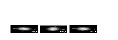
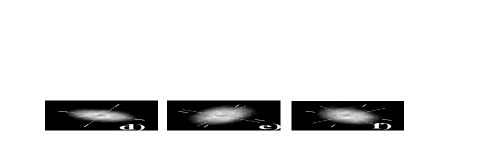
FIG. 11.: Transverse oscillations of a stirred condensate with $3.7\times 10^{5}$ atoms in an elongated trap with $\omega_{\perp}/2\pi=171$ Hz. For (a)-(c), the stirring frequency $\Omega/2\pi=114$ Hz is below the threshold for vortex nucleation, whereas for (d)-(f), the stirring frequency $\Omega/2\pi=120$ Hz has nucleated a vortex (visible at the center of the condensate). The sequences of pictures correspond to time delays $\tau=1,3$ and $5$ ms for which the ellipticity in the $xy$ plane is maximum. The fixed axes indicate the excitation basis of the quadrupole mode and the rotating ones indicate the condensate axes.

(Taken from Ref. [36]).

One should note that the vortex-induced splitting of the condensate modes is maximum if the vortex is located at the trap center. If a straight vortex line is displaced a distance $\zeta_{0}=r_{0}/R_{\perp}$ from the $z$ axis of the TF condensate, then the splitting of the quadrupole mode ($m=\pm 2$) is given by the expression

$$\omega_{+}-\omega_{-}=7\omega_{\perp}\frac{d_{\perp}^{2}}{R_{\perp}^{2}}\left(1-\frac{5}{4}\zeta_{0}^{2}\left[1+\frac{1}{2}\zeta_{0}^{4}-\zeta_{0}^{6}+\frac{3}{10}\zeta_{0}^{8}\right]\right)$$ (80)

The splitting goes to zero if the vortex moves out of the condensate ($\zeta_{0}=1$).

4 Numerical analysis for general interaction parameter

García-Ripoll and Pérez-García [102] have performed extensive numerical analyses of the stability of vortices in axisymmetric traps with an axial asymmetry parameter $\lambda=\omega_{z}/\omega_{\perp}=1$ (a sphere) and $\lambda=\frac{1}{2}$ (one particular cigar-shape condensate). They conclude that a doubly quantized vortex line has normal modes with imaginary frequencies and that an external rotation cannot stabilize it. For a singly quantized vortex in a spherical trap, however, they confirm the presence of one negative-frequency (anomalous) mode with $|\omega_{a}|<\Omega_{c}$. For their cigar-shape condensate, they find additional negative-frequency modes and suggest that such elongated condensates are less stable than spherical or disk-shape ones. More recent numerical work [116, 83] confirms these findings for other geometries, especially that for the ENS experiment [34], where the axial asymmetry is large ($\omega_{\perp}/\omega_{z}\approx R_{z}/R_{\perp}\approx 14$). It is expected that a vortex in an elongated condensate becomes stable only for an external angular velocity $\Omega_{m}=\max|\omega_{a}|$, where $\max|\omega_{a}|$ is the absolute value of the most negative of these anomalous modes. For only modestly elongated traps, the metastable frequency $\Omega_{m}$ exceeds the thermodynamic critical value $\Omega_{c}$; these results provide an alternative explanation of the ENS observation that the first vortex appears at an applied rotation $\approx 70\%$ higher than $\Omega_{c}$. Independently, an analysis of the bending modes of a trapped vortex [117] in the TF limit finds that a vortex in a spherical or disk-shape condensate has only one negative frequency (anomalous) mode, but the number of such modes in an elongated condensate increases with the axial asymmetry ratio $R_{z}/R_{\perp}$ (discussed below in Sec. V.D.2).

V Vortex dynamics

The preceding sections considered the equilibrium and stability of a vortex in a trapped Bose condensate, using the stationary GP equation and the Bogoliubov equations that characterize the small perturbations of the stationary vortex. These approaches are somewhat indirect, for they do not consider the dynamical motion of the vortex core. The present section treats two different methods that address such questions directly.

A Time-dependent Variational Analysis

Consider a variational problem for the action $\int dt\,{\cal L}(t)$ obtained from the Lagrangian

$${\cal L}(t)=\int dV\,\left[\frac{i\hbar}{2}\left(\Psi^{*}\,\frac{\partial\Psi}{\partial t}-\Psi\,\frac{\partial\Psi^{*}}{\partial t}\right)-\Psi^{*}\left(T+V_{{\rm tr}}-\Omega L_{z}\right)\Psi-\frac{1}{2}g\,|\Psi|^{4}\right].$$ (81)

It is easy to verify that the Euler-Lagrange equation for this action is precisely the time-dependent GP equation in the rotating frame.

If, instead of $\Psi({\bf r},t)$, we substitute a trial function that contains different variational parameters (for example, the location of the vortex core), the resulting time evolution of these parameters characterizes the dynamics of the condensate. This method is not exact, but it provides an appealing physical picture. For example, it determined the low-energy excitations of a trapped vortex-free condensate at zero temperature [118, 119] for general values of the interaction parameter. In the TF limit, this work reproduced the expressions derived by Stringari [57] based on Eq. (33).

1 Near-ideal regime

In the near-ideal limit, only the axisymmetric case has been studied, and it is natural to start from the noninteracting vortex state (36), incorporating small lateral displacements of the vortex and the center of mass of the condensate, along with a phase that characterizes the velocity field induced by the motion of the condensate [120]. In addition to the rigid dipole mode (in which the condensate and the vortex oscillate together at the transverse trap frequency $\omega_{\perp}$), an extra normal mode arises at the anomalous (negative) frequency $\omega_{a}$ given in Eq. (75) omitting the second-order corrections that are beyond the present approximation. In this weak-coupling limit, the resulting displacement of the vortex is twice that of the center of mass, so that both must be included to obtain the correct dynamical motion. Detailed analysis confirms the positive normalization and relative displacements found from the Bogoliubov equations for the same axisymmetric trap [113].

2 Thomas-Fermi regime for straight vortex in disk-shape trap

For a nonaxisymmetric trap in the TF regime, only the nonrotating case ($\Omega=0$) has been analyzed, using the fully anisotropic TF wave function as an appropriate trial state, again with parameters describing the small displacements of the straight vortex and the center of mass of the condensate [78]. The trial wave function was chosen in the form

$$\Psi\left({\bf r},t\right)=B(t)f\left[{\bf r}-{\mathchoice{{\hbox{\boldmath$\displaystyle r$}}}{{\hbox{\boldmath$\textstyle r$}}}{{\hbox{\boldmath$\scriptstyle r$}}}{{\hbox{\boldmath$\scriptscriptstyle r$}}}}_{0}(t)\right]F[{\bf r}-{\mathchoice{{\hbox{\boldmath$\displaystyle\eta$}}}{{\hbox{\boldmath$\textstyle\eta$}}}{{\hbox{\boldmath$\scriptstyle\eta$}}}{{\hbox{\boldmath$\scriptscriptstyle\eta$}}}}_{0}(t)]\prod_{j=x,y,z}\exp\left[ix_{j}\alpha_{j}(t)+ix_{j}^{2}\beta_{j}(t)\right].$$ (82)

Here the function $f\left({\bf r}\right)$ characterizes the vortex line inside the trap and far away from the vortex core has the approximate form $f\left({\bf r}\right)=e^{i\phi}$; the function $F({\bf r})$ is the TF condensate density. The time-dependent vector ${\mathchoice{{\hbox{\boldmath$\displaystyle\eta$}}}{{\hbox{\boldmath$\textstyle\eta$}}}{{\hbox{\boldmath$\scriptstyle\eta$}}}{{\hbox{\boldmath$\scriptscriptstyle\eta$}}}}_{0}(t)=(\eta_{0x},\eta_{0y},\eta_{0z})$ describes the motion of the center of the condensate, while ${\mathchoice{{\hbox{\boldmath$\displaystyle r$}}}{{\hbox{\boldmath$\textstyle r$}}}{{\hbox{\boldmath$\scriptstyle r$}}}{{\hbox{\boldmath$\scriptscriptstyle r$}}}}_{0}(t)=(x_{0},y_{0},0)$ describes the motion of the vortex line in the $xy$ plane. The other variational parameters are the amplitude $B(t)$ and the set $\alpha_{j}(t)$ and $\beta_{j}(t)$. Substitution of the trial wave function into (81) yields an effective Lagrangian as a function of the variational parameters (and their first time derivatives). The resulting Lagrangian equations have a solution that corresponds to the motion of the vortex relative to the condensate. For this solution the vortex motion is described by

$$x_{0}=\varepsilon_{0}R_{x}\sin\left(\omega_{a}t+\phi_{0}\right),\quad y_{0}=\varepsilon_{0}\,R_{y}\cos\left(\omega_{a}t+\phi_{0}\right),$$ (83)

while the displacement of the condensate is given by

$$\eta_{0x}=-\frac{15\varepsilon_{0}\xi^{2}}{2R_{y}}\ln\left(\frac{R_{\perp}}{\xi}\right)\frac{R_{x}}{R_{x}+R_{y}}\sin\left(\omega_{a}t+\phi_{0}\right),$$ (84)

$$\eta_{0y}=-\frac{15\varepsilon_{0}\xi^{2}\,}{2R_{x}}\ln\left(\frac{R_{\perp}}{\xi}\right)\frac{R_{y}}{R_{x}+R_{y}}\cos\left(\omega_{a}t+\phi_{0}\right),$$ (85)

where

$$\omega_{a}=-\frac{3\hbar\omega_{x}\omega_{y}}{4\mu}\ln\left(\frac{R_{\perp}}{\xi}\right)=-\frac{3\hbar}{2MR_{x}R_{y}}\ln\left(\frac{R_{\perp}}{\xi}\right),$$ (86)

in agreement with that found in Eq. (78). The quantity $x_{0}^{2}/R_{x}^{2}+y_{0}^{2}/R_{y}^{2}=\varepsilon_{0}^{2}$ remains constant as the vortex line follows an elliptic trajectory around the center of a trap along the line $V_{{\rm tr}}=const$, and the energy of the system is conserved [as follows from Eq. (49)]. The condensate also precesses with the relative phase shift $\pi$ at the same frequency, but the amplitude of the condensate motion is smaller than that of the vortex line by a factor $\sim\xi^{2}\ln\left(R_{\perp}/|q|\xi\right)/R_{x}R_{y}$.

For an axisymmetric TF condensate in rotational equilibrium at an angular velocity $\Omega$, the Lagrangian (81) provides a more general result for the precession frequency. With the hydrodynamic variables $\Psi=e^{iS}|\Psi|$, the first term of the Lagrangian becomes $-\hbar\int dV\,|\Psi|^{2}\partial S/\partial t$. Since the TF condensate density vanishes at the surface, the particle current also vanishes there, and it usually suffices to assume a single straight vortex displaced laterally to ${\bf r}_{0}(t)$, with $S({\bf r,r}_{0})=\arctan[(y-y_{0})/(x-x_{0})]$ and no image vortex. The Lagrangian becomes

$${\cal L}=\int dV\,Mn({\bf r})\,\dot{{\bf r}}_{0}\cdot{\bf v}_{0}({\bf r})-E(r_{0})+\Omega L_{z}(r_{0}),$$ (87)

where

$${\bf v}_{0}({\bf r})=\frac{\hbar}{M}\mathchoice{{\hbox{\boldmath$\displaystyle\nabla$}}}{{\hbox{\boldmath$\textstyle\nabla$}}}{{\hbox{\boldmath$\scriptstyle\nabla$}}}{{\hbox{\boldmath$\scriptscriptstyle\nabla$}}}S({\bf r,r}_{0})=-\frac{\hbar}{M}\mathchoice{{\hbox{\boldmath$\displaystyle\nabla$}}}{{\hbox{\boldmath$\textstyle\nabla$}}}{{\hbox{\boldmath$\scriptstyle\nabla$}}}{{\hbox{\boldmath$\scriptscriptstyle\nabla$}}}_{0}S({\bf r,r}_{0})=(\kappa/2\pi)\,\frac{\hat{z}\times({\bf r-r}_{0})}{|{\bf r-r}_{0}|^{2}}$$ (88)

is the circulating velocity field about the vortex line. In the special case of a two-dimensional condensate with the TF density $n(r)=n(0)(1-r_{\perp}^{2}/R_{\perp}^{2})$ per unit length, Eq. (87) becomes

$${\cal L}_{2}=(\dot{\phi}_{0}+\Omega)L_{z2}(r_{0})-\dot{\phi}_{0}L_{z2}(0)-E_{2}(r_{0}),$$ (89)

where $\phi_{0}$ is the azimuth angle describing position of the vortex line,

$$L_{z2}(r_{0})=\frac{1}{2}n(0)\pi R_{\perp}^{2}\hbar(1-\zeta_{0}^{2})^{2}$$ (90)

and

$$E_{2}(r_{0})=\frac{\kappa^{2}Mn(0)}{8\pi}\left[2(1-\zeta_{0}^{2})\ln\left(\frac{R_{\perp}}{\xi}\right)+(1-\zeta_{0}^{2})\ln(1-\zeta_{0}^{2})-1+2\zeta_{0}^{2}\right]$$ (91)

with $\zeta_{0}=r_{0}/R_{\perp}$ [note that $\frac{1}{2}n(0)$ is the mean particle density $\overline{n}$ per unit length]. These expressions differ from the classical results for a uniform fluid in a rotating cylinder [88, 121] because of the parabolic TF density; in particular, the TF angular momentum per unit length $L_{z2}$ here is proportional to $(1-\zeta_{0}^{2})^{2}$, whereas that for a uniform density is proportional to $1-\zeta_{0}^{2}$.

The Lagrangian dynamical equations show that the vortex precesses at fixed $r_{0}$ with the angular frequency

$$\dot{\phi}_{0}=-\Omega+\frac{\partial E_{2}/\partial r_{0}}{\partial L_{z2}/\partial r_{0}}=-\Omega-\frac{\partial E_{2}/\partial r_{0}}{\kappa Mr_{0}n(r_{0})}.$$ (92)

This result is just that expected from the Magnus force on a straight vortex [122, 123, 124]. For small displacements from the center, the precession frequency in a nonrotating two-dimensional condensate reduces to $\dot{\phi}_{0}\approx(\kappa/2\pi R_{\perp}^{2})\ln(R_{\perp}/\xi)\approx\frac{1}{2}\Omega_{c}$ [70], but $\dot{\phi}_{0}$ increases with increasing $r_{0}$ and eventually diverges near the edge of the condensate where the density vanishes.

The corresponding results for a three-dimensional disk-shape TF condensate follow from Eqs. (49) and (87). In particular, the integration over $z$ means that the total angular momentum $L_{z3}=N\hbar(1-\zeta_{0}^{2})^{5/2}$ associated with the presence of the vortex differs from the two-dimensional result proportional to $(1-\zeta_{0}^{2})^{2}$. Apart from numerical factors reflecting the three-dimensional geometry, Eq. (92) remains correct. For a straight vortex, it yields

$$\dot{\phi}_{0}=-\Omega+\frac{\Omega_{m}}{1-r_{0}^{2}/R_{\perp}^{2}},$$ (93)

where $\Omega_{m}=\frac{3}{2}(\hbar/MR_{\perp}^{2})\ln(R_{\perp}/\xi)$ is the metastable frequency (51) for the appearance of a central vortex in a disk-shape condensate. In the special case of a vortex near the center ($r_{0}\to 0$), this precession frequency reduces to (minus) the corresponding anomalous frequency $\omega_{a}(\Omega)$ in Eq. (78) for a condensate with a single central vortex line. To understand why the precession frequency $\dot{\phi}_{0}$ is the negative of the anomalous frequency, recall that the linearized perturbation in the density for the anomalous mode is proportional to $\exp i[m_{a}\phi-\omega_{a}(\Omega)t]=\exp i[-\phi-\omega_{a}(\Omega)t]$ because $m_{a}=-1$; this latter form shows clearly that the normal mode propagates around the symmetry axis at an angular frequency $-\omega_{a}(\Omega)$, with the sense of rotation fixed by the sign of $-\omega_{a}(\Omega)$.

According to (93), for a nonrotating trap the precession velocity of a displaced vortex increases with the vortex displacement as $v=\Omega_{m}r_{0}/(1-r_{0}^{2}/R_{\perp}^{2})$. It is interesting to estimate at what displacement the vortex velocity becomes supersonic [125]. Assuming the speed of sound varies radially with the local density as $c=c_{0}\sqrt{1-r_{0}^{2}/R_{\perp}^{2}}$, where $c_{0}=\sqrt{\mu/M}=\omega_{\perp}R_{\perp}/\sqrt{2}$, we obtain $v/c=(\sqrt{2}\Omega_{m}r_{0}/\omega_{\perp}R_{\perp})(1-r_{0}^{2}/R_{\perp}^{2})^{-3/2}$. As a result, the vortex velocity becomes supersonic if

$$\frac{r_{0}}{R_{\perp}}>{\frac{\omega_{\perp}}{\sqrt{2}\Omega_{m}}}\left(1-\frac{r_{0}^{2}}{R_{\perp}^{2}}\right)^{3/2}=\frac{\sqrt{2}R_{\perp}}{3\xi\ln(R_{\perp}/\xi)}\left(1-\frac{r_{0}^{2}}{R_{\perp}^{2}}\right)^{3/2}.$$ (94)

For parameters of JILA experiments [37] $R_{\perp}/\xi\approx 33$, this gives a critical displacement of $r_{0}/R_{\perp}\approx 0.82$ where the precession vortex velocity becomes supersonic.

B Method of Matched Asymptotic Expansions

At zero temperature, the dynamics of a condensate in a rotating nonaxisymmetric trap follows from the appropriate time-dependent GP equation

$$i\hbar\frac{\partial\Psi}{\partial t}=\left(-\frac{\hbar^{2}\nabla^{2}}{2M}+V_{{\rm tr}}+g|\Psi|^{2}-\mu(\Omega)+i\hbar\mathchoice{{\hbox{\boldmath$\displaystyle\Omega$}}}{{\hbox{\boldmath$\textstyle\Omega$}}}{{\hbox{\boldmath$\scriptstyle\Omega$}}}{{\hbox{\boldmath$\scriptscriptstyle\Omega$}}}\cdot({\bf r}\times\mathchoice{{\hbox{\boldmath$\displaystyle\nabla$}}}{{\hbox{\boldmath$\textstyle\nabla$}}}{{\hbox{\boldmath$\scriptstyle\nabla$}}}{{\hbox{\boldmath$\scriptscriptstyle\nabla$}}})\right)\Psi.$$ (95)

A vortex line in the condensate will, in general, move in response to the effect of the nonuniform trap potential and the external rotation, as well as self-induced effects caused by its own local curvature. This problem can be solved in the case of a large condensate, where the TF separation of length scales means that the vortex-core radius $\xi$ is much smaller than the condensate radii $R_{j}$. The relevant mathematics involves the method of matched asymptotic expansions [126, 127, 128].

1 Dynamics of straight vortex in Thomas-Fermi regime for disk-shape trap

As an introduction to these techniques, it is helpful first to concentrate on the case of a straight singly quantized vortex line [78], which is applicable to disk-shape condensates with $R_{z}\ll R_{\perp}$; this analysis generalizes two-dimensional results found by Rubinstein and Pismen [127]. Assume that the vortex is located near the center of the trap at a transverse position ${\bf r}_{\perp 0}(t)$. In this region, the trap potential does not change significantly on a length scale comparable with the vortex core size $\xi$. The method of matched asymptotic expansions compares the solution of Eq. (95) on two very different length scales:

First, consider the detailed structure of the vortex core. Assume that the vortex moves with a transverse velocity ${\bf V}\perp\hat{z}$, and transform to a co-moving frame centered at the vortex core. Away from the trap center, the trap potential exerts a force proportional to $\mathchoice{{\hbox{\boldmath$\displaystyle\nabla$}}}{{\hbox{\boldmath$\textstyle\nabla$}}}{{\hbox{\boldmath$\scriptstyle\nabla$}}}{{\hbox{\boldmath$\scriptscriptstyle\nabla$}}}_{\perp}V_{{\rm tr}}$ evaluated at the position ${\bf r}_{\perp 0}(t)$. The resulting steady solution includes the “asymptotic” region $|{\bf r}_{\perp}-{\bf r}_{\perp 0}|\gg\xi$.

Second, consider the region far from the vortex (on this scale, the vortex core is effectively a singularity). The short-distance behavior of this latter solution also includes the region $\xi\ll|{\bf r}_{\perp}-{\bf r}_{\perp 0}|$. The requirement that the two solutions match in the overlapping region of validity determines the translational velocity ${\bf V}$ of the vortex line.

Unfortunately, the details become rather intricate, but the final answer is elegant and physical:

$${\bf V}=\frac{3\hbar}{4M\mu}\left[\ln\left(\frac{R_{\perp}}{\xi}\right)-\frac{8\mu\Omega}{3\hbar\left(\omega_{x}^{2}+\omega_{y}^{2}\right)}\right]\,\left(\hat{z}\times\mathchoice{{\hbox{\boldmath$\displaystyle\nabla$}}}{{\hbox{\boldmath$\textstyle\nabla$}}}{{\hbox{\boldmath$\scriptstyle\nabla$}}}{{\hbox{\boldmath$\scriptscriptstyle\nabla$}}}_{\perp}V_{{\rm tr}}\right)=\frac{3\hbar}{4M\mu}\left[\ln\left(\frac{R_{\perp}}{\xi}\right)-\frac{2MR_{\perp}^{2}\Omega}{3\hbar}\right]\,\left(\hat{z}\times\mathchoice{{\hbox{\boldmath$\displaystyle\nabla$}}}{{\hbox{\boldmath$\textstyle\nabla$}}}{{\hbox{\boldmath$\scriptstyle\nabla$}}}{{\hbox{\boldmath$\scriptscriptstyle\nabla$}}}_{\perp}V_{{\rm tr}}\right),$$ (96)

where $R_{\perp}$ for an asymmetric trap is defined in Eq. (50). This expression has several notable features.

(a) The motion is along the direction $\hat{z}\times\mathchoice{{\hbox{\boldmath$\displaystyle\nabla$}}}{{\hbox{\boldmath$\textstyle\nabla$}}}{{\hbox{\boldmath$\scriptstyle\nabla$}}}{{\hbox{\boldmath$\scriptscriptstyle\nabla$}}}_{\perp}V_{{\rm tr}}$ and hence follows an equipotential line of $V_{{\rm tr}}$. Thus the trajectory conserves energy, which is expected because the GP equation omits dissipative processes. In the present case of an anisotropic harmonic trap, the trajectory is elliptical.

(b) For a nonrotating trap ($\Omega=0$), the motion is counterclockwise in the positive sense at the frequency given by Eq. (86), proportional to $\omega_{x}\omega_{y}$.

(c) With increasing applied rotation $\Omega$, the translational velocity ${\bf V}$ decreases and vanishes at the special value

$$\Omega_{m}=\frac{3\hbar\left(\omega_{x}^{2}+\omega_{y}^{2}\right)}{8\mu}\ln\left(\frac{R_{\perp}}{\xi}\right)=\frac{3\hbar}{2MR_{\perp}^{2}}\ln\left(\frac{R_{\perp}}{\xi}\right),$$ (97)

proportional to $\frac{1}{2}\left(\omega_{x}^{2}+\omega_{y}^{2}\right)$. This value precisely reproduces Eq. (51) associated with the onset of metastability for small transverse displacements of the vortex from the trap center.

(d) For $\Omega>\Omega_{m}$, the motion is clockwise as seen in the rotating frame. A detailed analysis based on the normalization of the Bogoliubov amplitudes shows that the positive-norm state has a frequency [compare Eq. (86)]

$$\omega_{a}(\Omega)=\frac{2\omega_{x}\omega_{y}}{\omega_{x}^{2}+\omega_{y}^{2}}\left(\Omega-\Omega_{m}\right).$$ (98)

Note that this expression differs somewhat from Eq. (76) because the trap here is anisotropic. The normal-mode frequency is negative and hence unstable for $\Omega<\Omega_{m}$, but it becomes positive and hence stable for $\Omega>\Omega_{m}$. This direct analysis of the motion of a straight vortex reproduces the physics of the onset of (static) metastability (51) studied with the GP Hamiltonian and the (dynamic) anomalous mode (79) and (86) studied with the Bogoliubov equations and with the Lagrangian method.

2 Dynamics of curved vortex in Thomas-Fermi regime

Consider a nonaxisymmetric trap that rotates with an angular velocity $\textstyle\Omega$ (for convenience, $\textstyle\Omega$ is often taken along the $z$ axis). At low temperature in a frame rotating with the same angular velocity, the trap potential is time independent, and Eq. (95) describes the evolution of the condensate wave function. In the TF limit, the method of matched asymptotic expansions again yields an approximate solution for the motion of a singly quantized vortex line with instantaneous configuration ${\bf r}_{0}(z,t)$. Let $\hat{t}$ be the local tangent to the vortex (defined with the usual right-hand rule), $\hat{n}$ be the corresponding normal, and $\hat{b}\equiv\hat{t}\times\hat{n}$ be the binormal. A generalization of the work of Pismen and Rubinstein [126, 127] eventually yields the explicit expression for the local translational velocity of the vortex [117]

$${\bf V(r}_{0})=-\frac{\hbar}{2M}\left(\frac{\hat{t}\times{\mathchoice{{\hbox{\boldmath$\displaystyle\nabla$}}}{{\hbox{\boldmath$\textstyle\nabla$}}}{{\hbox{\boldmath$\scriptstyle\nabla$}}}{{\hbox{\boldmath$\scriptscriptstyle\nabla$}}}}V_{{\rm tr}}({\bf r}_{0})}{g|\Psi_{TF}|^{2}}+k\hat{b}\right)\ln\left(\xi\,\sqrt{\frac{1}{R_{\perp}^{2}}+\frac{k^{2}}{8}}\right)+\frac{2\,{\mathchoice{{\hbox{\boldmath$\displaystyle\nabla$}}}{{\hbox{\boldmath$\textstyle\nabla$}}}{{\hbox{\boldmath$\scriptstyle\nabla$}}}{{\hbox{\boldmath$\scriptscriptstyle\nabla$}}}}V_{{\rm tr}}({\bf r}_{0})\times{\mathchoice{{\hbox{\boldmath$\displaystyle\Omega$}}}{{\hbox{\boldmath$\textstyle\Omega$}}}{{\hbox{\boldmath$\scriptstyle\Omega$}}}{{\hbox{\boldmath$\scriptscriptstyle\Omega$}}}}}{\Delta_{\perp}V_{{\rm tr}}({\bf r}_{0})},$$ (99)

where $k$ is the local curvature (assumed small, with $k\xi\ll 1$) and $\Delta_{\perp}$ is the Laplacian operator in the plane perpendicular to ${\bf\Omega}$.

This vector expression holds for general orientation of the gradient of the trap potential, the normal to the vortex line, and the angular velocity vector. Near the TF boundary of the condensate, the denominator of the first term becomes small, implying that the numerator $\hat{t}\times{\mathchoice{{\hbox{\boldmath$\displaystyle\nabla$}}}{{\hbox{\boldmath$\textstyle\nabla$}}}{{\hbox{\boldmath$\scriptstyle\nabla$}}}{{\hbox{\boldmath$\scriptscriptstyle\nabla$}}}}\,V_{{\rm tr}}({\bf r}_{0})$ must also vanish near the boundary. As a result, the axis of the vortex line $\hat{t}$ is parallel to ${\mathchoice{{\hbox{\boldmath$\displaystyle\nabla$}}}{{\hbox{\boldmath$\textstyle\nabla$}}}{{\hbox{\boldmath$\scriptstyle\nabla$}}}{{\hbox{\boldmath$\scriptscriptstyle\nabla$}}}}V_{{\rm tr}}$ at the surface and hence obeys the intuitive boundary condition that the vortex must be perpendicular to the condensate surface.

C Normal modes of a vortex in a rotating two-dimensional TF condensate

This very general Eq. (99) applies in many different situations [117]. The simplest case is an initially straight vortex in a two-dimensional asymmetric TF condensate with ${\bf\Omega}=\Omega\hat{z}$ and $\omega_{z}=0$ (hence no confinement in the $z$ direction). For small displacements, the $x$ and $y$ coordinates of the vortex core execute harmonic motion $\propto\exp[i(\kappa z-\omega t)]$ that can vary between helical and planar depending on the relative phase of the $x$ and $y$ motion. The dispersion relation $\omega_{\kappa}(\Omega)$ depends on the continuous parameter $\kappa$ and the rotation frequency $\Omega$, along with the TF radii $R_{x}$ and $R_{y}$ [117]:

$$\omega_{\kappa}(\Omega)=\pm\frac{\hbar}{2MR_{x}R_{y}}\sqrt{\left(2-\kappa^{2}R_{x}^{2}-\tilde{\Omega}\right)\left(2-\kappa^{2}R_{y}^{2}-\tilde{\Omega}\right)}\ln\left(\xi\sqrt{\frac{1}{R_{\perp}^{2}}+\frac{|\kappa|^{2}}{8}}\right).$$ (100)

where

$$\tilde{\Omega}=\frac{4MR_{x}^{2}R_{y}^{2}}{\hbar(R_{x}^{2}+R_{y}^{2})\ln\left(\xi\sqrt{\frac{1}{R_{\perp}^{2}}+\frac{|\kappa|^{2}}{8}}\right)^{-1}}\Omega$$ (101)

is a dimensionless rotation speed.

Of all the various normal modes, a straight vortex line ($\kappa=0$) has the most negative (anomalous) frequency

$$\omega_{a}(\Omega)=-\frac{\hbar}{2MR_{x}R_{y}}\,\left[\ln\left(\frac{R_{\perp}}{\xi}\right)-\frac{4\mu\Omega}{\hbar\left(\omega_{x}^{2}+\omega_{y}^{2}\right)}\right],$$ (102)

where an analysis similar to that for Eq. (98) shows that the minus sign corresponds to the Bogoliubov solution with positive norm. For $\Omega=0$, the vortex precesses counterclockwise about the $z$ axis in the positive sense. With increasing rotation frequency $\Omega$, the precession frequency decreases and vanishes at $\Omega=\Omega_{m}$, where the metastable rotation frequency in two dimensions is

$$\Omega_{m}=\frac{\hbar\left(\omega_{x}^{2}+\omega_{y}^{2}\right)}{4\mu}\,\ln\left(\frac{R_{\perp}}{\xi}\right)=\frac{\hbar}{MR_{\perp}^{2}}\,\ln\left(\frac{R_{\perp}}{\xi}\right);$$ (103)

as expected, this value is the precession frequency $\frac{1}{2}\Omega_{c}$ discussed below Eq. (92) [compare Eq. (51) for $\Omega_{m}$ in a three-dimensional disk-shape TF condensate; the different numerical coefficient arises from the integration over the parabolic density in the $z$ direction].

More generally, for $\kappa^{2}>0$ and a nonaxisymmetric trap ($R_{x}>R_{y}$), the oscillation frequency can be imaginary (and hence unstable) within a range of axial wave numbers determined by $\sqrt{(2-\tilde{\Omega})}/R_{x}<|\kappa|<\sqrt{(2-\tilde{\Omega})}/R_{y}$. For sufficiently fast rotation, however, the frequencies become real, and the small oscillations become stable at a rotation frequency $\tilde{\Omega}>\tilde{\Omega}_{m}=2$. In the limit of a uniform unbounded condensate ($R_{x},R_{y}\to\infty$), the general dispersion relation reduces to the familiar one for helical waves on a long straight vortex line [7]

$$\omega=\pm\frac{\hbar}{2M}\,\kappa^{2}\ln\left(|\kappa|\xi\right).$$ (104)

Using this dispersion relation, Barenghi [129] estimated the amplitude of the vortex waves due to thermal excitation (the cloud is assumed to rotate at an angular velocity $\Omega>\Omega_{c}$, so that the vortex is stable). He showed that finite-temperature effects in a Bose condensate can distort the vortex state significantly, even at the very low temperatures relevant to the experiments. For $T=10^{-7}$ K, $\bar{n}\approx 10^{12}-10^{13}$ cm${}^{\!\!-3}$ and $R\approx 5\;\mu$m, the amplitude of vortex oscillations can be 4-14 times the size of the vortex core. At the same time, the thermal excitation of vortex waves in superfluid ⁴He is negligible (much smaller than the corresponding vortex-core size).

D Normal modes of a vortex in a rotating three-dimensional TF condensate

Consider a three-dimensional TF condensate with $\omega_{z}>0$, confined within a TF region $z^{2}\leq R_{z}^{2}=2\mu/M\omega_{z}^{2}$.

1 General formalism

For a vortex that initially lies along the $z$ axis, it is straightforward to find the pair of coupled equations for the small transverse displacements of the vortex $x(z,t)$ and $y(z,t)$. In particular, we seek solutions of the form

$$x=x(z)\sin(\omega t+\varphi_{0}),\qquad y=y(z)\cos(\omega t+\varphi_{0}),$$ (105)

in which case the amplitudes $x(z)$ and $y(z)$ describe the vortex shape and obey coupled ordinary differential equations. Introducing dimensionless scaled coordinates $x\to R_{x}x$, $y\to R_{y}y$, $z\to R_{z}z$, we find from Eq. (99)

$$\tilde{\omega}(1-z^{2})x=-\frac{d}{dz}\left[\beta(1-z^{2})\frac{dy}{dz}\right]-y+\tilde{\Omega}(1-z^{2})y,$$ (106)

$$\tilde{\omega}(1-z^{2})y=-\frac{d}{dz}\left[\alpha(1-z^{2})\frac{dx}{dz}\right]-x+\tilde{\Omega}(1-z^{2})x,$$ (107)

where

$$\alpha=\frac{R_{x}^{2}}{R_{z}^{2}},\quad\beta=\frac{R_{y}^{2}}{R_{z}^{2}}$$ (108)

characterize the trap anisotropy and

$$\tilde{\omega}=\frac{2MR_{x}R_{y}}{\hbar\,\ln(R_{\perp}/\xi)}\,\omega,\quad\tilde{\Omega}=\frac{4MR_{x}^{2}R_{y}^{2}}{\hbar(R_{x}^{2}+R_{y}^{2})\ln(R_{\perp}/\xi)}\,\Omega$$ (109)

are dimensionless angular velocities.

These equations (106) and (107) constitute a two-component Sturm-Liouville system with natural boundary conditions [130] because the factor $1-z^{2}$ vanishes at $z=\pm 1$. Consequently, the eigenfunctions merely must remain bounded at the surface of the condensate. A straightforward generalization of the usual analysis shows that the eigenfunctions obey the orthogonality condition

$$\int_{-1}^{1}dz\,(1-z^{2})x_{m}y_{n}\propto\delta_{mn}\,.$$ (110)

2 Special solutions

In the general case of a nonaxisymmetric trap, the resulting equations remain coupled, but they separate in the particular case of stationary solutions with $\omega=0$. For a nonrotating trap, such configurations reflect a balance between the effects of curvature and the nonuniform trap potential. For example, the small-amplitude stationary solutions $x_{n}(z)$ remain finite at the surface $z=\pm 1$ only for certain special values of the trap anisotropy

$$\alpha=\alpha_{n}=\frac{2}{n(n+1)},$$ (111)

where $n\geq 0$ is an integer. The corresponding solutions have the form $x_{n}(z)\propto P_{n}(z)$, where $P_{n}$ is the familiar Legendre polynomial. The solutions have $n$ nodes and cross the $z$ axis $n$ times. If $\alpha$ differs from one of these special values (111), there is no stationary configuration. Similarly, the equation for the $y$ displacement has stationary solutions only if $\beta\equiv R_{y}^{2}/R_{z}^{2}=2/[m(m+1)]$.

This classification of the solutions by the number of nodes remains more generally valid. In the special case of an axisymmetric condensate ($\alpha=\beta$), we can consider the precession frequency $\omega_{n}$ of the mode with $n$ nodes as a function of the axial trap anisotropy $\alpha$. Evidently, the function $\omega_{n}$ changes sign at the special value $\alpha=\alpha_{n}=2/[n(n+1)]$. This observation allows us to determine the number of modes with negative frequencies at a fixed value of the anisotropy parameter $\alpha$. For $\alpha\geq 1$ (a spherical or disk-shape condensate), only one mode has a negative frequency. If $\frac{1}{3}<\alpha<1$, there are two such anomalous modes, and so on. If $\alpha_{n}<\alpha<\alpha_{n-1}$, a nonrotating axisymmetric TF condensate has $n$ anomalous modes with negative frequency.

The special case of a nearly disk-shape anisotropic rotating TF condensate is particularly tractable because $\alpha^{-1}$ and $\beta^{-1}$ provide small expansion parameters. There is only one relevant normal mode, with frequency

$$\omega_{a}(\Omega)=-\Omega_{m}+\Omega,$$ (112)

where

$$\Omega_{m}=\frac{\hbar\left(\omega_{x}^{2}+\omega_{y}^{2}\right)}{8\mu}\left[3+\frac{1}{10}\left(\frac{1}{\alpha}+\frac{1}{\beta}\right)\right]\ln\left(\frac{R_{\perp}}{\xi}\right)\quad\hbox{for nearly disk-shape TF condensate}.$$ (113)

If $\Omega<\Omega_{m}=|\omega_{a}(0)|$, the frequency is negative, and the mode is therefore unstable. This value generalizes that found previously in Eqs. (51) and (97) for the angular velocity at which a straight vortex at the center of a thin disk-shape condensate becomes metastable, now including the first corrections of order $\alpha^{-1}$ and $\beta^{-1}$.

This result (113) remains approximately correct for a spherical condensate ($\alpha=\beta=1$), which is the geometry used in recent JILA experiments [37]. Since $\Omega_{m}$ is numerically equal to the frequency $|\omega_{a}|$ of the one anomalous mode in the nonrotating condensate, Eq. (113) also yields the precession frequency of a nearly straight vortex moving counterclockwise around the center of the condensate[78, 83]. In particular, we find $|\omega_{a}|/\omega=\frac{8}{5}(\xi/R)\ln(1.96R/\xi)$, where $\omega$ is the isotropic trap frequency and the additional numerical factor $1.96$ in the logarithm is the next correction to the logarithmic accuracy (see, for example, Ref. [127]). With the JILA parameters $R\approx 22\ \mu$m and $\xi\approx 0.67\ \mu$m, this expression yields $|\omega_{a}|/2\pi=1.58\pm 0.16$ Hz, where the uncertainty reflects the omission of corrections of relative order $(\xi/R)\ln(R/\xi)\approx 0.1$. For comparison, the experimental value $1.8\pm 0.1$ Hz for the precession frequency is somewhat larger, but the theoretical prediction is sensitive to the number $N$ of atoms in the condensate and, as seen in Eq. (93), to the radial displacement of the vortex [83, 123].

The situation is very different for an elongated cigar-shape condensate with $R_{z}\gg R_{\perp}$, when the solutions for the precessing normal-mode amplitudes grow exponentially with $|z|$. In contrast to the two-dimensional case, such solutions are now possible because the condensate is bounded along the $z$ axis. In the simplest case of an axisymmetric trap with $R_{x}=R_{y}=R_{\perp}$, the mode with no nodes has a frequency $\omega_{a}(\Omega)=-\Omega_{m}+\Omega$. Although this expression has the same form as Eq. (112) for a disk-shape condensate, the physical behavior is very different because the metastable angular velocity

$$\Omega_{m}=\frac{\hbar}{2MR_{\perp}^{2}}\,\frac{R_{z}^{2}}{R_{\perp}^{2}}\ln\left(\frac{R_{\perp}}{\xi}\right)\approx\frac{R_{z}^{2}}{5\,R_{\perp}^{2}}\,\Omega_{c}$$ (114)

becomes large for a highly elongated TF condensate. For the ENS geometry [34, 36], where $\omega_{\perp}/\omega_{z}\approx R_{z}/R_{\perp}\approx 14.4$, Eq. (114) is far too large to fit the observations and can even exceed the limit of rotational mechanical stability $\Omega=\omega_{\perp}$ that occurs when the centrifugal force cancels the confining trap potential.

For a harmonic transverse external potential $\propto r_{\perp}^{2}$, the method of matched asymptotic expansions is valid if the vortex displacement $r$ from the $z$ axis satisfies the condition $r\gtrsim\xi$ (in the vicinity of the vortex core the trap potential is approximated as a linear function). For a long cigar-shape condensate, the solution for the lowest mode has the form: $r=r_{0}\cosh(z/\alpha)$, where $r_{0}$ is the vortex displacement at $z=0$. The condition of small vortex displacement implies that $r_{0}\cosh(1/\alpha)\ll R_{\perp}$, while the condition of small vortex curvature $k\xi\ll 1$ implies that $r_{0}\xi\cosh(1/\alpha)/R_{z}^{2}\alpha^{2}\ll 1$. A combination of these conditions gives the following restriction on the validity Eq. (114): $\exp(1/\alpha)\ll 2R_{\perp}/\xi$. For the ENS experiments, $1/\alpha\approx 200$ and $R_{\perp}/\xi\approx 21$, so that this condition fails.

As mentioned in Sec. IV.D.4, the frequency for the onset of metastability $\Omega_{m}$ in Eq. (114) can be larger than the thermodynamic critical angular velocity $\Omega_{c}$ in Eq. (43). This behavior is readily understandable because $\Omega_{c}$ characterizes the energy of a straight vortex along the symmetry axis [compare Eq. (42)], whereas the most unstable normal-mode amplitude explicitly involves the small-amplitude distortion with no nodes. For a very elongated condensate, the resulting vortex dynamics is particularly sensitive to the large curvature of the condensate surface near the two ends of the symmetry axis (in contrast to the small curvature for the flattened condensate).

Recent numerical studies [116, 83] of the most negative anomalous modes for a trap geometry corresponding to the ENS experiments [34, 36] yield values of $\Omega_{m}$ that are significantly smaller than the prediction given in Eq. (114). Reference [116] mentions the possible failure of the TF picture in the transverse direction, even though the conventional TF ratio $R_{\perp}/\xi$ is large, at least near the plane $z=0$. As confirmation of the validity of the GP equation and the particular role of the anomalous modes, the numerically determined [83] $\Omega_{m}/2\pi\approx 0.73\nu_{\perp}\approx 124$ Hz agrees well with the ENS value $\Omega_{{\rm obs}}/2\pi\approx 120$ Hz for the appearance of the first vortex.

For an axisymmetric trap ($\alpha=\beta$), we can seek normal-mode solutions in the form $x(z)=y(z)$, leaving a single equation

$$\left[\tilde{\omega}(\tilde{\Omega})-\tilde{\Omega}\right](1-z^{2})x=-\frac{d}{dz}\left[\alpha(1-z^{2})\frac{dx}{dz}\right]-x$$ (115)

that depends only on the Doppler-shifted frequency $\tilde{\omega}(\tilde{\Omega})-\tilde{\Omega}=\tilde{\omega}(0)$. The eigenfunctions are even or odd functions of $z$ and can be classified by the number of times the vortex crosses the $z$ axis (the number of nodes), $m=0,1,2,\cdots$. Figure 12 shows the dimensionless frequency $\tilde{\omega}(0)$ as a function of the trap anisotropy $\alpha=R_{\perp}^{2}/R_{z}^{2}$ for $m=0,1$, and $2$. In agreement with the analytical results, a disk-shape trap ($\alpha\geq 1$) has only a single mode with negative frequency $\tilde{\omega}_{0}$. For $\frac{1}{3}<\alpha<1$, there are two such modes ($m=0$ and $m=1$) and successively more negative-frequency modes appear for smaller $\alpha$. As noted previously, the critical frequency $\tilde{\Omega}_{m}$ for metastability is $|\tilde{\omega}_{0}|$, which is smaller than $\tilde{\Omega}_{c}$ for disk-shape traps and for moderately elongated traps. Our numerical analysis for the present TF limit predicts that $\tilde{\Omega}_{m}\geq\tilde{\Omega}_{c}$ for $\alpha=R_{\perp}^{2}/R_{z}^{2}\leq 0.26$, which is somewhat larger than the value $0.2$ implied by the limiting expression in Eq. (114).

FIG. 12.: Dimensionless frequencies $\tilde{\omega}\equiv\tilde{\omega}(\Omega=0)$ for the first three normal modes of a vortex in an axisymmetric trap as a function of the axial anisotropy $\alpha=R_{\perp}^{2}/R_{z}^{2}$. The lower horizontal line is the negative of the dimensionless thermodynamic critical angular velocity $\tilde{\Omega}_{c}=5$. Note that $|\tilde{\omega}_{0}|>\tilde{\Omega}_{c}$ for $\alpha<0.26$.

As in the case of a two-dimensional condensate, the frequency of the anomalous modes can become imaginary for an anisotropic trap with $R_{x}\neq R_{y}$ [117]. To demonstrate that result, let us consider Eqs. (106) and (107) for a trap close to axisymmetric with $|\alpha-\beta|\ll\alpha$. The eigenfrequencies of the axisymmetric trap [with $\alpha=\beta=\alpha_{0}=\frac{1}{2}(\alpha+\beta)$] are real and have the form $\tilde{\omega}_{m}(\tilde{\Omega})=\tilde{\omega}_{m}+\tilde{\Omega}$, where $m=0,1,2,\cdots$ denotes the various modes. For an anomalous mode, the frequency $\tilde{\omega}_{m}$ is negative, and the eigenfrequency $\tilde{\omega}_{m}(\tilde{\Omega})$ is equal to zero if the trap rotates with the angular velocity $\tilde{\Omega}=|\tilde{\omega}_{m}|$. One can rewrite Eqs. (106) and (107) as follows:

$$\tilde{\omega}(1-z^{2})\pmatrix{x\cr y\cr}=\hat{H}_{0}\pmatrix{x\cr y\cr}+\hat{V}\pmatrix{x\cr y\cr},$$ (116)

where

$$\hat{H}_{0}=\left\{-2-\alpha_{0}\partial_{z}[(1-z^{2})\partial_{z}]+(1-z^{2})|\tilde{\omega}_{m}|\right\}\pmatrix{0&1\cr 1&0\cr},$$

$$\hat{V}=-\partial_{z}[(1-z^{2})\partial_{z}]\pmatrix{0&\beta-\alpha_{0}\cr\alpha-\alpha_{0}&0\cr}+(1-z^{2})(\tilde{\Omega}-|\tilde{\omega}_{m}|)\pmatrix{0&1\cr 1&0\cr}.$$

Considering $\hat{V}$ as a perturbation, we obtain the following expression for the normal-mode frequency in a nonaxisymmetric trap:

$$\tilde{\omega}=\pm\sqrt{\left(|\tilde{\omega}_{m}|-|\alpha-\beta|I_{m}-\tilde{\Omega}\right)\left(|\tilde{\omega}_{m}|+|\alpha-\beta|I_{m}-\tilde{\Omega}\right)},$$ (117)

where

$$I_{m}=\frac{\int_{-1}^{1}dz(1-z^{2})\left(\partial_{z}x_{m}\right)^{2}}{2\int_{-1}^{1}(1-z^{2})x_{m}^{2}dz}>0$$ (118)

and $x_{m}=x_{m}(z)$ describes shape of the $m$th vortex mode. As we increase the trap rotation, the eigenfrequency is real for $\tilde{\Omega}<|\tilde{\omega}_{m}|-I_{m}|\alpha-\beta|$ . Then, when $|\tilde{\Omega}-|\tilde{\omega}_{m}||<I_{m}|\alpha-\beta|$, the frequency becomes imaginary. Finally, if $\tilde{\Omega}>|\tilde{\omega}_{m}|+I_{m}|\alpha-\beta|$, the frequency again becomes real. For a given trap anisotropy (given $\alpha$ and $\beta$), one or several normal modes of the vortex have negative frequency. Trap rotation $\tilde{\Omega}$ shifts the frequencies in the positive direction. When the frequency of a normal mode in the rotating frame approaches zero, the frequency becomes imaginary until $|\tilde{\omega}_{m}+\tilde{\Omega}|=I_{m}|\alpha-\beta|$. If we increase the trap rotation further, the frequency (in the rotating frame) becomes positive.

For a disc-shape condensate (with $\alpha_{0}\gg 1$) there is only one anomalous mode with $x_{a}=y_{a}=\varepsilon\left(1+{z^{2}}/{2\alpha_{0}}\right)$ and $\tilde{\omega}_{a}=-3-\frac{1}{5}\alpha_{0}^{-1}$. For a nonaxisymmetric rotating trap, the frequency of this mode becomes imaginary in the interval $|\tilde{\Omega}-|\tilde{\omega}_{a}||<\epsilon|\tilde{\omega}_{a}|/(15\alpha_{0})$, where $\epsilon=|R_{x}-R_{y}|/R_{x}$ is the trap anisotropy in the transverse direction. Thus for a disk-shape condensate (with $\alpha_{0}\gg 1$), the solution has an imaginary frequency in a relatively narrow range of trap rotation.

For a cigar-shape condensate, several normal modes have negative frequencies. In the limit $\alpha_{0}\ll 1$, the solution for the lowest anomalous mode has the form $x_{a}=y_{a}=\varepsilon\cosh\left(z/\alpha_{0}\right)$ and $\tilde{\omega}_{a}\approx-1/\alpha_{0}$. Consequently, the frequency is imaginary if $|\tilde{\Omega}-|\tilde{\omega}_{a}||<\epsilon|\tilde{\omega}_{a}|$, namely in a relatively wide range of trap rotation. If the transverse trap anisotropy is large enough, several different anomalous normal modes can have imaginary frequencies in the same range of angular velocities. In this case a vortex along the $z$ axis is stable (there are no normal modes with imaginary frequencies) only if the trap rotates slightly faster than the frequency of the lowest anomalous mode. This behavior could be relevant to ENS experiments.

3 Energy of a curved trapped vortex

Consider a trap that contains a singly quantized vortex and rotates with angular velocity $\Omega$ about the $z$ axis. At zero temperature, Eq. (99) governs the dynamics of each element of the line

$${\bf V(r})=-\frac{\hbar}{2M}\left(\frac{\hat{t}\times{\mathchoice{{\hbox{\boldmath$\displaystyle\nabla$}}}{{\hbox{\boldmath$\textstyle\nabla$}}}{{\hbox{\boldmath$\scriptstyle\nabla$}}}{{\hbox{\boldmath$\scriptscriptstyle\nabla$}}}}V_{{\rm tr}}({\bf r})}{g|\Psi_{TF}|^{2}}+k\hat{b}\right)\ln\left(\xi\,\sqrt{\frac{1}{R_{\perp}^{2}}+\frac{k^{2}}{8}}\right)+\frac{2\,{\mathchoice{{\hbox{\boldmath$\displaystyle\nabla$}}}{{\hbox{\boldmath$\textstyle\nabla$}}}{{\hbox{\boldmath$\scriptstyle\nabla$}}}{{\hbox{\boldmath$\scriptscriptstyle\nabla$}}}}V_{{\rm tr}}({\bf r})\times{\mathchoice{{\hbox{\boldmath$\displaystyle\Omega$}}}{{\hbox{\boldmath$\textstyle\Omega$}}}{{\hbox{\boldmath$\scriptstyle\Omega$}}}{{\hbox{\boldmath$\scriptscriptstyle\Omega$}}}}}{\Delta_{\perp}V_{{\rm tr}}({\bf r})},$$ (119)

where ${\bf r=(}x(z),y(z),z)$ determines the shape of the line. Correspondingly, Eq. (40) serves as the energy functional

$$E(\Psi)=\int dV\left(\frac{\hbar^{2}}{2M}|\nabla\Psi|^{2}+V_{{\rm tr}}|\Psi|^{2}+\frac{1}{2}g|\Psi|^{4}+\Psi^{*}i\hbar\Omega\frac{\partial\Psi}{\partial\phi}\right)$$ (120)

in the rotating frame (for simplicity, we now use $E$ instead of $E^{\prime}$). In Sec. III.B, a physically motivated wave function served to evaluate Eq. (120), yielding Eq. (49) for the energy of a straight vortex displaced laterally from the trap axis. As noted previously, the assumption of a straight vortex restricted the analysis to a disk-shape condensate.

To find the energy of a curved vortex, one can first find the condensate wave function $\Psi$ and then substitute it into the functional (120). For a curved vortex line, however, this approach is complicated. Instead, one can use Eq. (119) to find the vortex energy directly. As we know, the stationary Gross-Pitaevskii equation can be obtained by varying the energy functional (120). The dynamical equation (119) is, in fact, the time dependent Gross-Pitaevskii equation, written in a way suitable to describe the vortex motion. Consequently, if we formally put ${\bf V(r)=0}$ in Eq. (119) (namely omit the time derivatives), then the resulting stationary equation must be an extremum of the energy functional $E_{V}$ associated with the presence of the vortex and considered as a functional of the vortex shape $E_{V}=E_{V}\left(x(z),y(z)\right)$. An equivalent energy functional has the form (in the TF limit):

$$E_{V}\left(x(z),y(z)\right)=\frac{\pi\hbar^{2}}{M}\int dz\,\left[|\Psi_{TF}|^{2}\sqrt{1+(x^{\prime})^{2}+(y^{\prime})^{2}}\ln\left(\frac{R_{\perp}}{\xi}\right)-\frac{2M}{\hbar}\frac{g|\Psi_{TF}|^{4}\Omega}{\Delta_{\perp}V_{{\rm tr}}}\right],$$ (121)

where the prime denotes the derivative with respect to $z$. Variation of Eq. (121) with respect to $x(z)$ and $y(z)$ gives Eq. (119) with ${\bf V(r)=0}$, apart from terms of higher order $xx^{\prime}{}^{2},xy^{\prime}{}^{2},\cdots$ . Hence Eq. (121) provides an energy functional for the small deformations of a vortex about a straight configuration along the $z$ axis (when the fourth-order terms in the displacement can be omitted) or for arbitrary displacements of a straight vortex. Note that Eq. (121) involves only a one-dimensional line integral instead of the three-dimensional expression in Eq. (120), which is a significant simplification. In scaled dimensionless units $x\to R_{x}x$, etc., this energy functional becomes

$$E_{V}\left(x(z),y(z)\right)=2\pi\mu R_{z}\xi^{2}n(0)\int dz\,\left[\left(1-x^{2}-y^{2}-z^{2}\right)\sqrt{1+\alpha(x^{\prime})^{2}+\beta(y^{\prime})^{2}}\ln\left(\frac{R_{\perp}}{\xi}\right)-\frac{2\mu\Omega(1-x^{2}-y^{2}-z^{2})^{2}}{\hbar(\omega_{x}^{2}+\omega_{y}^{2})}\right],$$ (122)

where $n(0)=\mu/g$ is the density at the center of the vortex-free condensate, $\xi^{2}=\hbar^{2}/2M\mu$ and the integration is restricted to the region $1-x^{2}-y^{2}-z^{2}\geq 0$. Using Eq. (122) one can obtain a simple expression for the angular momentum of the condensate in the presence of a curved vortex line:

$$L_{z}=-\frac{\partial E_{V}}{\partial\Omega}=\frac{15}{8}\hbar N\frac{R_{x}R_{y}}{R_{x}^{2}+R_{y}^{2}}\int dz(1-x^{2}-y^{2}-z^{2})^{2},$$ (123)

where $N=8\pi R_{x}R_{y}R_{z}n(0)/15$ is the total number of particles in the condensate.

The integration in Eq. (122) is particularly easy for a straight vortex and readily reproduces Eq. (49). An expansion for small lateral displacements yields Eqs. (51) and (52) for $\Omega_{m}$ and $\Omega_{c}$ for a disk-shape TF condensate. In the more general case of arbitrary small displacements, Eq. (122) can be expanded to second order in the amplitudes $x$ and $y$ and their derivatives. Use of the dynamical equations that lead to (106) and (107) gives the simple expression

$$E_{V}\left(x(z),y(z)\right)=\frac{8\pi}{3}\mu R_{z}\,\xi^{2}n(0)\left[\ln\left(\frac{R_{\perp}}{\xi}\right)-\frac{8}{5}\,\frac{\mu\Omega}{\hbar\left(\omega_{x}^{2}+\omega_{y}^{2}\right)}\right]+\frac{15}{8}\hbar N\int_{-1}^{1}dz\,(1-z^{2})(x\dot{y}-y\dot{x}),$$ (124)

The first term of Eq. (124) reproduces the value of $\Omega_{c}$ for a general TF condensate, and the second term becomes a sum over all normal modes of the form (105)

$$E_{V}\left(x(z),y(z)\right)=\frac{8\pi}{3}\mu R_{z}\,\xi^{2}n(0)\left[\ln\left(\frac{R_{\perp}}{\xi}\right)-\frac{8}{5}\,\frac{\mu\Omega}{\hbar\left(\omega_{x}^{2}+\omega_{y}^{2}\right)}\right]+\frac{15}{8}N\sum_{n}\hbar\omega_{n}(\Omega)\int_{-1}^{1}dz\,(1-z^{2})x_{n}(z)y_{n}(z),$$ (125)

where the orthogonality condition Eq. (110) eliminates the cross terms between different normal modes. If any of the normal modes is anomalous (namely with negative frequency), then the system is unstable with respect to excitation of those modes. This analysis confirms the interpretation of $\Omega_{m}$ as the applied rotation frequency at which the frequency of the last anomalous mode vanishes in the rotating frame. At this applied $\Omega$ the location of the vortex line along the $z$ axis becomes a local minimum of energy. Note that this conclusion is wholly equivalent to that in Eq. (64) based on the Bogoliubov quasiparticles.

One should note that for a cigar-shape condensate with $R_{z}\gtrsim 2R_{\perp}$, there is an interval of angular velocity of trap rotation when $\Omega_{c}<\Omega<\Omega_{m}$. In this interval, the frequency of (at least) the lowest vortex mode remains negative, but penetration of a vortex into the condensate is energetically favorable. Under such a condition, the vortex line can lower its energy by undergoing a finite-amplitude deformation, and the ground state of the system corresponds to a curved vortex line displaced from the trap axis (see also [116]).

4 Precession and tilting of a straight vortex line in a nearly spherical TF condensate

The preceding discussion of vortex dynamics in a three-dimensional confined condensate has focused on the small-amplitude displacements from equilibrium. In the special case of a spherical trap, however, the presence of a zero-frequency precessing mode (Sec. V.D.2) allows a more general analysis of the nonlinear dynamics, which is directly relevant to recent JILA experiments on the evolution of an initially straight vortex in a nearly spherical TF condensate [92]. In practice, the trap deviates slightly from spherical with $R_{x}\neq R_{y}\neq R_{z}$.

For a spherical condensate, a motionless straight singly quantized vortex through the center of trap satisfies the general Eq. (99) for the velocity of a vortex line because the axis of the vortex $\hat{t}$ lies along $\mathchoice{{\hbox{\boldmath$\displaystyle\nabla$}}}{{\hbox{\boldmath$\textstyle\nabla$}}}{{\hbox{\boldmath$\scriptstyle\nabla$}}}{{\hbox{\boldmath$\scriptscriptstyle\nabla$}}}V_{{\rm tr}}$. Let

$$x=\gamma_{x}s,\quad y=\gamma_{y}s,\quad z=\gamma_{z}s$$ (126)

specify the axis of the vortex line, where $s$ is the arc length measured from the trap center and ($\gamma_{x}$, $\gamma_{y}$, $\gamma_{z}$) are the direction cosines relative to the principal axes of the anisotropic trap. For small anisotropy, the vortex remains approximately straight, but the direction cosines become time dependent. To first order in the anisotropy, the curvature $k$ can be omitted in Eq. (99) and $|\Psi_{TF}|^{2}$ can be approximated by the TF density for a spherical vortex-free condensate with TF radius $R$. Standard perturbation theory yields the nonlinear dynamical equations

$$\dot{\gamma}_{x}=\frac{5\hbar}{4\mu}\ln\left(\frac{R}{\xi}\right)\left(\omega_{z}^{2}-\omega_{y}^{2}\right)\gamma_{y}\gamma_{z},$$ (127)

$$\dot{\gamma}_{y}=\frac{5\hbar}{4\mu}\ln\left(\frac{R}{\xi}\right)\left(\omega_{x}^{2}-\omega_{z}^{2}\right)\gamma_{z}\gamma_{x},$$ (128)

$$\dot{\gamma}_{z}=\frac{5\hbar}{4\mu}\ln\left(\frac{R}{\xi}\right)\left(\omega_{y}^{2}-\omega_{x}^{2}\right)\gamma_{x}\gamma_{y}.$$ (129)

This set of equations is familiar in classical mechanics as Euler’s equations for the torque-free motion of a rigid body [131, 132, 133], where they describe the motion of the angular-velocity vector as seen in the body-fixed frame. In the present context, this set of three coupled nonlinear equations has two first integrals

$$\gamma_{z}^{2}+\gamma_{y}^{2}+\gamma_{z}^{2}=1,$$ (130)

which verifies that the first-order anisotropy simply rotates the vortex axis and

$$\omega_{x}^{2}\gamma_{z}^{2}+\omega_{y}^{2}\gamma_{y}^{2}+\omega_{z}^{2}\gamma_{z}^{2}={\rm const},$$ (131)

which is the condition of energy conservation.

The simplest situation is an axisymmetric trap with $\omega_{x}=\omega_{y}=\omega_{\perp}$, in which case the vortex line precesses uniformly about the $z$ axis (the symmetry axis) at a fixed polar angle $\arccos\gamma_{z}(0)$ at a frequency [117]

$$\omega=\frac{5\hbar(\omega_{z}^{2}-\omega_{\perp}^{2})}{4\mu}\,\gamma_{z}(0)\ln\left(\frac{1.96R}{\xi}\right)=\frac{5\hbar}{2M}\left(\frac{1}{R_{z}^{2}}-\frac{1}{R_{\perp}^{2}}\right)\,\gamma_{z}(0)\ln\left(\frac{1.96R}{\xi}\right),$$ (132)

where the numerical factor 1.96 inside the logarithm is the same as that discussed below Eq. (113). For positive (negative) $\omega$, the precession is counter-clockwise (clockwise). Recent experiments at JILA have observed two recurrences of such precessional motion in a slightly flattened trap with $\omega_{z}-\omega_{\perp}\approx 0.1\omega_{z}$ and a polar tipping angle of $45^{\circ}$ from the $z$ axis. In this case, Eq. (132) predicts $\omega/2\pi\approx 0.33\pm 0.03$ Hz, in an agreement with the observed value $0.25\pm 0.02$ Hz [92].

More generally, for an anisotropic trap (with $\omega_{x}>\omega_{y}>\omega_{z}$), the vortex executes closed trajectories (see Fig. 13). For initial positions close to the $x$ and $z$ axes (the smallest and largest TF radii), the motion is “stable,” remaining nearby, but small-amplitude motion about an initial position close to the $y$ axis (the intermediate TF radius) yields imaginary frequencies. Thus such trajectories deviate far from the initial neighborhood, even though they eventually return (this periodic behavior is familiar from the corresponding solutions of the Euler equations [131, 132, 133]). Reference [117] gives explicit solutions for the resulting dynamical motion of a nearly straight vortex in a totally anisotropic trap.

FIG. 13.: Typical trajectories of the end of a straight vortex line (that passes through the condensate center) during its motion in a slightly nonspherical trap with $R_{x}<R_{y}<R_{z}$.

VI Effect of thermal quasiparticles, vortex lifetime and dissipation

In previous sections we considered a Bose condensate within the Bogoliubov approximation, which omits the effect of thermal quasiparticles. At finite temperatures, however, these noncondensate atoms can modify the frequencies of the vortex modes and dissipate energy.

A Bogoliubov and Hartree-Fock-Bogoliubov Theories

Let us consider a condensate in thermal equilibrium at temperature $T$. Within the Hartree-Fock Bogoliubov (HFB) theory, the condensate wave function $\Psi$ satisfies the following generalized Gross-Pitaevskii equation (in a frame rotating with the angular velocity $\Omega\hat{z}$)[134]:

$$\left(-\frac{\hbar^{2}}{2M}\nabla^{2}+V_{{\rm tr}}+g|\Psi|^{2}+2g\rho({\bf r})-\mu(\Omega)+i\hbar\Omega\partial_{\phi}\right)\Psi+g\Delta({\bf r})\Psi^{*}=0,$$ (133)

where $\phi$ is the azimuthal angle in cylindrical polar coordinates, $\rho({\bf r})$ is the density of the noncondensed gas and $\Delta({\bf r})$ is the anomalous average of two Bose field operators describing the noncondensate (as in Sec. IV.A, $\hat{\psi}=\Psi+\hat{\phi}$ is the quantum field operator, with $\Delta=\langle\hat{\phi}\hat{\phi}\rangle$ and $\rho=\langle\hat{\phi}^{\dagger}\hat{\phi}\rangle$). The collective excitation energies $E$ of the system are the eigenvalues of the generalized Bogoliubov equations for the coupled amplitudes $u({\bf r})$ and $v({\bf r})$

$$\left(-\frac{\hbar^{2}}{2M}\nabla^{2}+V_{{\rm tr}}+2g|\Psi|^{2}+2g\rho({\bf r})-\mu(\Omega)\right)\pmatrix{u\cr v}$$

$$+\pmatrix{i\hbar\Omega\partial_{\phi}&-g\left[\Delta({\bf r})+\Psi{}^{2}\right]\cr-g\left[\Delta^{*}({\bf r})+\Psi^{*}{}^{2}\right]&-i\hbar\Omega\partial_{\phi}}\pmatrix{u\cr v}=E\pmatrix{u\cr-v}.$$ (134)

Eq. (134) is valid at least for temperatures much less than the chemical potential $\mu$ when resonant contributions (the so-called Szepfalusy-Kondor processes) to the self-energies are not substantial [135]. In addition, we have self-consistency relations for the noncondensate density $\rho({\bf r})$

$$\rho({\bf r})=\sum_{n}\left[\frac{|u_{n}({\bf r})|^{2}+|v_{n}({\bf r})|^{2}}{\exp(E_{n}/k_{B}T)-1}+|v_{n}({\bf r})|^{2}\right],$$ (135)

and for the anomalous average $\Delta({\bf r})$

$$\Delta({\bf r})=-\sum_{n}\left[\frac{2u_{n}({\bf r})v_{n}^{*}({\bf r})}{\exp(E_{n}/k_{B}T)-1}+u_{n}({\bf r})v_{n}^{*}({\bf r})\right],$$ (136)

where $n$ denotes quantum numbers specifying the excited states with energies $E_{n}$ ($n=0,1,2,\cdots$ ). The eigenfunctions $u_{n}({\bf r})$ and $v_{m}({\bf r})$ satisfy the normalization condition:

$$\int\left[u_{n}^{*}({\bf r})u_{m}({\bf r})-v_{n}^{*}({\bf r})v_{m}({\bf r})\right]d{\bf r}=\delta_{nm}.$$ (137)

Equations (133)-(137) constitute a complete set of the self-consistent equations for the HFB theory. Within this theory, the quasiparticle eigenvalues $E_{n}$ in Eqs. (134)-(136) must be positive because the condensate is defined to have zero energy. Thus a negative eigenvalue means a failure of the self-consistency and the associated thermal equilibrium of the system. If $\rho({\bf r})$ and $\Delta({\bf r})$ are set to zero, we recover the Bogoliubov theory. If we set only $\Delta({\bf r})=0$, we obtain the Popov approximation. For a vortex-free condensate in the low-temperature limit, the Popov and Bogoliubov theories give identical excitation spectra [138]. The excitation spectrum in the HFB theory has an unphysical gap because it does not treat all condensate-condensate interactions consistently [134]. Gapless modifications of the HFB theory, the so-called G1 and G2 approximations, are discussed in [139, 140]. Normally, the zero-temperature limit of the Popov, G1 and G2 theories should be the Bogoliubov theory (which does not take into account noncondensate atoms). For a non rotating condensate with a vortex, however, this is not the case because vortex is unstable.

Within the Bogoliubov theory, an isolated vortex in a nonrotating harmonic trap has at least one normal mode with negative energy. Let us apply the HFB theory for a condensate with a vortex. To find a self-consistent solution for the lowest eigenvalue at low temperatures, one can use a perturbation method analogous to those developed in Ref. [114]. We consider a condensate in an axisymmetric trap that rotates with an angular velocity $\Omega$ around the $z$ axis. We assume that the condensate contains a singly quantized vortex along the $z$ axis. For simplicity we consider a disk-shape condensate, so one can omit vortex curvature in investigating the lowest normal mode. The condensate wave function has the form $\Psi=e^{i\phi}|\Psi|$, with $\Delta=e^{2i\phi}|\Delta|$, and we can rewrite the generalized Bogoliubov equations as:

$$\hat{H}_{0}\pmatrix{u\cr v}+\hat{V}\pmatrix{u\cr v}=E\pmatrix{u\cr-v},$$ (138)

where

$$\hat{H}_{0}=\left(-\frac{\hbar^{2}}{2M}\nabla^{2}+\frac{1}{2}M\omega_{z}^{2}z^{2}+2g|\Psi_{0}|^{2}-\mu(\Omega)\right)\pmatrix{1&0\cr 0&1}+\pmatrix{i\hbar\Omega\partial_{\phi}&-g\Psi_{0}{}^{2}\cr-g\Psi_{0}^{*}{}^{2}&-i\hbar\Omega\partial_{\phi}},$$ (139)

and $\hat{V}$ includes the remaining part of Eq. (134). Here, $\Psi_{0}$ is the wave function for an unbounded condensate in the $xy$ plane with the same chemical potential; its excitations obey the equation

$$\hat{H}_{0}\pmatrix{u_{0}\cr v_{0}}=E\pmatrix{u_{0}\cr-v_{0}}.$$ (140)

Equation (140) has an exact pair of solutions (see Ref. [114]) with positive norm and energy

$$E_{0}=\hbar\Omega.$$ (141)

Let us now make the following assumption: $E_{0}\ll k_{B}T\ll E_{1},E_{2},\cdots$, where $E_{0}$ is the energy of the lowest normal mode, which can depend on $T$. Then the term with $n=0$ gives the main contribution in the sum in Eqs. (135), (136), and we obtain:

$$\rho({\bf r})\approx\frac{k_{B}T}{E_{0}}\left[|u_{0}({\bf r})|^{2}+|v_{0}({\bf r})|^{2}\right]$$ (142)

$$\Delta({\bf r})\approx-\frac{2k_{B}T}{E_{0}}u_{0}({\bf r})v_{0}^{*}({\bf r})$$ (143)

For a singly quantized vortex one can derive the expression

$$\rho(r_{\perp}=0,z)\approx\frac{1.44\mu k_{B}T}{E_{0}I^{2}g\xi^{2}}\left(1-\frac{z^{2}}{R_{z}^{2}}\right),$$ (144)

where $I^{2}\approx 16\sqrt{2}\pi\mu^{3/2}/3g\omega_{z}\sqrt{M}$ is a normalization integral, and

$$|\Delta(r_{\perp}=0,z)|\approx 0.$$ (145)

In first-order perturbation theory, the lowest energy eigenvalue $E_{0}$ is defined by the equation:

$$E_{0}=\hbar\Omega+E_{a}\left(\frac{\gamma k_{B}T}{E_{0}}-1\right),$$ (146)

where $E_{a}=(3\hbar^{2}\omega_{\perp}^{2}/4\mu)\ln\left(R_{\perp}/\xi\right)$ and $\gamma=0.077R_{\perp}^{4}/N\xi^{4}$ are positive with $N=\frac{8}{15}\pi n(0)R_{z}R_{\perp}^{2}$ the total number of particles in the condensate, and $\mu$ can be taken as the chemical potential for a nonrotating trap. Eq. (146) has two solutions, one with positive energy and one with negative energy that reproduces the previous anomalous mode with $E_{0}=\hbar\Omega-E_{a}$ as $T\rightarrow 0$. The negative solution can be formally omitted, satisfying the requirement of self-consistency. The positive solution has the form:

$$E_{0}=\frac{1}{2}\left[\sqrt{(E_{a}-\hbar\Omega)^{2}+4E_{a}\gamma k_{B}T}-(E_{a}-\hbar\Omega)\right].$$ (147)

For nonrotating trap ($\Omega=0$), we find

$$E_{0}=\frac{E_{a}}{2}\left[\sqrt{1+\frac{4\gamma k_{B}T}{E_{a}}}-1\right].$$ (148)

If $T\rightarrow 0$, we obtain $E_{0}\approx\gamma k_{B}T$, so that $E_{0}$ is proportional to $T$ in the low-temperature limit. In fact our method generalizes the Beliaev theory [136] for the vortex state. Recently Pitaevskii and Stringari actually generalized the Beliaev approach (in the density-phase representation) for the trapped Thomas-Fermi condensate [137].

Virtanen, Simula and Salomaa made numerical calculations of vortex normal modes at finite $T$ within the Popov, G1 and G2 approximations and demonstrated that for a singly quantized vortex there is a self-consistent solution with only positive frequencies in the limit $T\rightarrow 0$ [141]. Their lowest energy solution corresponds to our Eq. (148). The vortex mode (148) arises from the presence of quasiparticles (an external pinning potential can also result in such motion [142]). At low temperatures, the quasiparticles are mostly localized in the vortex-core region and provide an extra repulsive potential [the term $2g\rho({\bf r})$ in Eq. (134)] that affects the elementary excitations. At $T=0$, the residual localized noncondensate fraction arises from the interaction between particles; this result follows from Eq. (144) if we take $E_{0}\propto T$ at low temperatures. The additional potential has a peak at the vortex core and the vortex line precesses around the quasiparticle potential center with a positive excitation energy.

However, this does not mean that quasiparticles stabilize the vortex in a trap. The physics of the problem is the following. At any moment during the vortex motion, quasiparticles fill the vortex core (the relaxation time of quasiparticles is much less than the period of the vortex precession). The vortex line participates in two motions: first, the vortex precesses around the trap center with the frequency $\hbar\omega_{a}=-E_{a}<0$ ($\Omega=0$). The trap potential is responsible for this unstable mode. The quasiparticles are localized in the vortex core and move together with the vortex; their presence simply slightly changes the chemical potential and slightly decreases the normal mode frequency. In second motion, the vortex line moves around the center of mass of the quasiparticles in a locally uniform condensate (in $xy$ plane). The amplitude of this motion is less than $\xi$ and the frequency can be found from Eq. (148) in the limit $R_{x},R_{y}\rightarrow\infty$ or $E_{a}\rightarrow 0$:

$$\hbar\omega_{T}=\sqrt{\gamma E_{a}k_{B}T}=0.37\sqrt{\frac{\mu k_{B}T}{n_{0}R_{z}\xi^{2}}\ln\left(\frac{R_{\perp}}{\xi}\right)},$$ (149)

where $n_{0}$ is the density of the vortex free condensate at the vortex location (in the plane $z=0$). For JILA parameters $\gamma\approx 0.3$, $E_{a}\approx 1.58$Hz, then for $T=0.8T_{c}$ we obtain $\omega_{T}\approx 13.6$ Hz. If this mode is thermally excited, its amplitude is given by

$$A=\xi\left(\frac{6a}{R_{z}}\right)^{1/2}\left(\frac{k_{B}T}{\hbar\omega_{T}}\right)^{1/2},$$ (150)

where $a$ is the scattering length. For parameters of JILA experiments $A=0.16\xi$. Taking into account $\omega_{T}\propto\sqrt{T}$ we obtain the following temperature dependence $A\propto T^{1/4}$. It is interesting to note that the thermal mode (149) exists only in 3D condensate; in the limit $R_{z}=\infty$ both the mode frequency and the amplitude go to zero.

Recent measurements of the lowest vortex modes in the JILA experiments are in a good quantitative agreement with solutions of the time-dependent Gross-Pitaevskii equation [37, 83, 117]. The JILA experiments measure, in fact, not only the absolute value, but also the sign of the lowest vortex mode. The negative value of the anomalous-mode frequency means that the vortex precesses in the same direction as the superfluid flow around the vortex core, which is seen in the experiments. An experimental observation of the thermal mode (149) could be next challenging problem of future investigations.

B Dissipation and Vortex Lifetimes

It is valuable to consider dissipation and its role in the vortex lifetime. In a nonrotating trap, the ground state of the system is a vortex-free condensate, so that a condensate with a vortex necessarily constitutes an excited state. In the absence of dissipation, however, the vortex line moves along trajectories of constant energy, remaining inside the condensate. The condensate with a vortex will be unstable only if there is a mechanism to transfer the system to the lower-energy vortex-free state [97]. The dissipative dynamics of a straight vortex due to its interaction with the thermal cloud in a trapped Bose-condensed gas was discussed by Fedichev and Shlyapnikov [143]. If the vortex line moves with respect to the normal component, scattering of elementary excitations by the vortex produces a friction force, like that in superfluid ⁴He (see Ch. 3 of Ref. [14]). Such a mechanism can transfer energy and momentum to the thermal cloud. The friction force ${\bf F}$ can be decomposed into longitudinal and transverse components: ${\bf F}=-D{\bf u}-D^{\prime}({\bf u}\times\hat{n}),$ where ${\bf u}$ is the velocity of the vortex line with respect to the normal component, $D$ and $D^{\prime}$ are the longitudinal and transverse friction coefficients, respectively, and $\hat{n}$ is a local tangent vector to the vortex line. The transverse friction coefficient is independent of the scattering amplitude and is given by the universal expression $D^{\prime}=\hbar\rho_{n}/M$, where $\rho_{n}$ is the local mass density of the normal component [144]. The longitudinal friction coefficient depends on the scattering process. In the limit $k_{B}T\gg\mu$, one can treat the elementary excitations as single particles, with the result that $\rho_{n}\approx 0.1M^{5/2}T^{3/2}/\hbar^{3}$ and the longitudinal friction coefficient is proportional to the temperature: $D\approx\hbar n\,(na^{3})^{1/2}T/\mu$, where $n=|\Psi|^{2}$ is the superfluid density for the vortex-free condensate and $a$ is the $s$-wave scattering length [143].

In the presence of dissipation, the vortex line moves toward a (local) minimum of the energy. In a nonrotating condensate, an off-center vortex precesses around the trap center and is expected to spiral out to the condensate boundary due to the dissipation. Once the vortex reaches the boundary, it presumably decays by emitting phonons and single-particle excitations. The radial motion of the vortex is governed by the longitudinal friction coefficient: $v_{r}\approx Du/\hbar n\approx(na^{3})^{1/2}Tu/\mu\ll u$, where $u$ is the precessional speed. Using this expression, one can estimate the characteristic lifetime of the vortex state [143]. At present, no dissipation of the moving vortex has been observed in the JILA experiments [37]. A characteristic decay time for the dissipative mechanism of Fedichev and Shlyapnikov in the JILA conditions is significantly larger than the life-time of the condensate. The temperature and density are too small to see the dissipation.

Another factor that can influence the vortex lifetime is the possibility that a moving vortex can emit phonons. It is known that a moving vortex in an infinite compressible fluid emits phonons, leading to a slow loss of energy [145]. Recently,  Lundh and Ao [123] studied the radiation of sound from a moving vortex in an infinite, uniform system. A homogeneous two-dimensional superfluid described by a nonlinear Schrödinger equation is equivalent to (2+1)-dimensional electrodynamics, with vortices playing the role of charges and sound corresponding to electromagnetic radiation [146, 147]. Thus, a vortex moving on a circular trajectory in an infinite superfluid radiates sound waves, which are analogous to the cyclotron radiation of an electrical charge moving along a circular orbit. The power radiated by a vortex with unit length executing circular motion with frequency $\omega$ at a radius $r_{0}$ is given by the following Poynting vector [123]:

$$P=\frac{\pi Q^{2}\omega^{3}r_{0}^{2}}{4c_{s}^{2}},$$ (151)

where $Q=-\hbar\sqrt{2\pi n/M}$ is the “vortex charge,” $n$ is the uniform superfluid density, and $c_{s}=\sqrt{\mu/M}$ is the velocity of sound.

In a nonuniform system, such as a two-dimensional or a disk-shape axisymmetric trapped condensate, an off-center vortex performs a circular motion around the symmetry axis. If such motion excites sound waves (radiates energy), the vortex will move outward toward regions of lower potential energy, until it eventually escapes from the cloud. In a trapped condensate, however, the excitations all remain confined within the condensate, and no phonon radiation is expected. In particular, the wavelength $\lambda$ of sound that would be emitted exceeds the size $R$ of the condensate. Indeed, $\lambda\sim 2\pi c_{s}/\omega$ and the precession frequency of the straight vortex is of the order of $\omega\sim\hbar\ln(R/\xi)/MR^{2}$; as a result, $\lambda/R\sim(R/\xi)\ln(R/\xi)\gg 1$, and the “cyclotron” radiation is prohibited.

Finally, let us discuss how vortex generation affects the dissipation in superfluids. One classic manifestation of superfluidity is that objects traveling below a critical velocity propagate through a superfluid without dissipation. According to the Landau criterion [105], which relies on the use of Galilean invariance, the critical velocity is $v_{L}=\min[E(p)/p]$, where $E(p)$ is the energy of an elementary excitation with momentum $p$. For a homogeneous Bose condensate, the Bogoliubov spectrum implies a Landau critical velocity equal to the speed of sound $v_{L}=c_{s}$. The Landau critical velocity can usually be observed only by moving microscopic particles through the superfluid. Such motion of microscopic impurities through a trapped gaseous Bose condensate was studied recently in [148]. As the impurities traverse the condensate, they dissipate energy by colliding with the stationary condensate and radiating phonons. When the impurity velocity was reduced below the speed of sound, however, the collision probability decreased dramatically, providing evidence for superfluidity in the condensate.

If a macroscopic object moves through the condensate, dissipation can occur due to turbulence and vortex formation in the superfluid, even if the object’s velocity is much lower than the Landau critical velocity. Recently, dissipation in a Bose-Einstein condensed gas was studied by moving a blue-detuned laser beam through the condensate [149, 150]. The laser beam repels atoms from its focus and creates a moving macroscopic “hole” in the condensate. The observed heating of the system agrees with the prediction of dissipation when the flow field becomes locally supersonic. Numerical simulations of the nonlinear Schrödinger equation were used to study the flow field around an object moving through a homogeneous condensate [28, 151, 152, 153, 122]. When the object moves faster than a critical velocity $v_{c}$, these studies show that the superfluid flow becomes unstable against the formation of quantized vortex lines, which gives rise to a new dissipative regime. Pairs of vortices with opposite circulation are generated at opposite sides of the object. The rate of the energy transfer to the condensate by the moving object increases significantly above this critical velocity for vortex formation. The heating rate can be expressed as $dE/dt=E_{{\rm pair}}f_{s}$, where $E_{{\rm pair}}$ is the energy of a vortex pair and $f_{s}$ is the shedding frequency. The rate of vortex-pair shedding $f_{s}$ is proportional to $v-v_{c}$ and thus larger when the speed of sound is lower.

Other simulations of the GP equation have demonstrated that vortex-antivortex pairs or vortex half-rings can be generated by superflow around a stationary obstacle [152, 154, 155, 28] or through a small aperture [156]. One might expect similar excitations in a rotating condensate. In addition, vortex half-rings can be nucleated at the condensate surface when the local tangential velocity exceeds a critical value.

VII Vortex states in mixtures and Spinor condensates

The advent of multicomponent BECs [157, 158, 159] has provided many new possibilities for quantum-mechanical state engineering. Since there is no intrinsic difficulty in loading and cooling more than one alkali element in the same trap, interpenetrating superfluids can now be realized experimentally. Binary mixtures of condensates can consist of different alkalis, or different isotopes, or different hyperfine states of the same alkali atom. Such binary mixtures of Bose condensates have a great variety of ground states and vortex structures that are experimentally accessible by varying the relative particle numbers of different alkalis [6]. In particular, one can move continuously from regimes of interpenetrating superfluids to those with separated phases. Many alkali binary mixtures contain a coexistence region, which is the analog of ³He-⁴He interpenetrating superfluids in ultralow-temperature physics [160].

A Basic Phenomena

Most experiments on Bose-Einstein condensation of atomic gases of ⁸⁷Rb[1], ⁷Li[2], and ²³Na[3] have used magnetic traps to condense atoms with a hyperfine spin $F=2$ (or $F=1$). Such a condensate of spin-$F$ bosons constitutes a spinor field

$$\langle\hat{\psi}_{m}({\bf r},t)\rangle=\zeta_{m}({\bf r},t)\Psi({\bf r},t),$$ (152)

where $\hat{\psi}_{m}$ is the field operator, $m$ labels $F_{z}$ (where $-F\leq m\leq F$), $\Psi$ is a scalar, and $\zeta_{m}$ is a normalized spinor. In magnetic traps, the spins of the alkali atoms are frozen and maximally aligned with the local magnetic field ${\bf B}$ [6]. As a result, $\zeta$ is given by the eigenvalue equation $\hat{{\bf B}}\cdot{\bf F}\zeta=F\zeta$, where ${\bf F}$ is the hyperfine spin operator and $\hat{{\bf B}}$ is a unit vector along ${\bf B}$. The dynamics of $\langle\hat{\psi}_{m}\rangle$ is therefore completely specified by the scalar field $\Psi$, as in ⁴He. Thus, even though the alkali atoms carry a spin, they behave in magnetic traps like scalar particles. In contrast to the scalar field, however, the spinor field in Eq. (152) possesses a local spin-gauge symmetry: a local gauge change $\exp[i\chi({\bf r},t)]$ of $\langle\hat{\psi}_{m}\rangle$ can be undone by a local spin rotation $\exp[-i(\chi/F)\hat{{\bf B}}({\bf r},t)\cdot{\bf F}]$. Because of this symmetry, the effective Hamiltonian of the scalar field $\Psi$ is not that of ⁴He, but that of a neutral superfluid in a velocity field ${\bf u}_{s}$. The velocity (or gauge field) ${\bf u}_{s}$ is a direct reflection of the spin-gauge symmetry and it is given by

$${\bf u}_{s}=-\frac{i\hbar}{M}\zeta^{\dagger}{\mathchoice{{\hbox{\boldmath$\displaystyle\nabla$}}}{{\hbox{\boldmath$\textstyle\nabla$}}}{{\hbox{\boldmath$\scriptstyle\nabla$}}}{{\hbox{\boldmath$\scriptscriptstyle\nabla$}}}}\zeta.$$ (153)

The velocity ${\bf u}_{s}$ can be calculated from the vorticity ${\bf\Omega}_{s}$ of ${\bf u}_{s}$, which satisfies the Mermin-Ho relation[161, 162],

$${\bf\Omega}_{s}=\frac{1}{2}{\mathchoice{{\hbox{\boldmath$\displaystyle\nabla$}}}{{\hbox{\boldmath$\textstyle\nabla$}}}{{\hbox{\boldmath$\scriptstyle\nabla$}}}{{\hbox{\boldmath$\scriptscriptstyle\nabla$}}}}\times{\bf u}_{s}=\left(\frac{\hbar}{2M}\right)\epsilon_{\alpha\beta\gamma}\hat{B}_{\alpha}{\mathchoice{{\hbox{\boldmath$\displaystyle\nabla$}}}{{\hbox{\boldmath$\textstyle\nabla$}}}{{\hbox{\boldmath$\scriptstyle\nabla$}}}{{\hbox{\boldmath$\scriptscriptstyle\nabla$}}}}\hat{B}_{\beta}\times{\mathchoice{{\hbox{\boldmath$\displaystyle\nabla$}}}{{\hbox{\boldmath$\textstyle\nabla$}}}{{\hbox{\boldmath$\scriptstyle\nabla$}}}{{\hbox{\boldmath$\scriptscriptstyle\nabla$}}}}\hat{B}_{\gamma}.$$ (154)

Equation (154) shows that the spatial variations of ${\bf B}$ necessary to produce the trapping potential will inevitably generate a nonvanishing superfluid velocity ${\bf u}_{s}=(2\hbar/M)\left(1-B_{z}/B\right){\mathchoice{{\hbox{\boldmath$\displaystyle\nabla$}}}{{\hbox{\boldmath$\textstyle\nabla$}}}{{\hbox{\boldmath$\scriptstyle\nabla$}}}{{\hbox{\boldmath$\scriptscriptstyle\nabla$}}}}\,[\arctan\,(B_{y}/B_{x})]$ [6]. If ${\bf B}_{0}=B_{0}\hat{z}$ is the magnetic field at the center of an axisymmetric harmonic trap and $\omega_{0}$ is the maximum trap frequency, then the spin-gauge effect generates the following constant effective “rotation” $\Omega_{s}$ around the $\hat{z}$ axis [6]:

$$\,\frac{{\bf\Omega}_{s}}{\omega_{0}}\sim-\hat{z}\,\frac{\hbar\omega_{0}}{\mu_{B}B_{0}},$$ (155)

where $\mu_{B}$ is the Bohr magneton. The superfluid velocity ${\bf u}_{s}$ splits the degeneracy of the harmonic energy levels, breaks the inversion symmetry of the vortex-nucleation angular velocity $\Omega_{c}$, and can produce vortex ground states in the absence of external rotation if $\Omega_{s}>\Omega_{c}$ [6]. In current experiments, the spin-gauge effect is small; for example, if $\omega_{0}=10$ Hz and $B_{0}=1$ G, we obtain $\Omega_{s}/\omega_{0}\sim 10^{-5}$. In oblate traps with $\omega_{z}\gg\omega_{\perp}$, however, the spin-gauge effect can be significant ($\Omega_{s}$ could be comparable with $\omega_{\perp}$ for large enough values of $\omega_{z}$).

Recently, the MIT group has succeeded in trapping a ²³Na Bose condensate by purely optical means [158, 159]. In contrast to a magnetic trap, the spins of the alkali atoms in such an optical trap are essentially free, so that the spinor nature of the alkali Bose condensate can be fully realized. Specifically, ²³Na atoms possess a hyperfine spin, with $F=1$ in the lower multiplet. All three possible projections of the hyperfine spin can be optically trapped simultaneously. Thus the condensate is described by a spin-1 spinor. The internal vortex structure of a trapped spin-1 BEC was investigated in Ref. [163]. Such vortices and their stability were also discussed in [20, 164]. In an optical trap, the ground state of spin-1 bosons such as ²³Na, ³⁹K, and ⁸⁷Rb can be either ferromagnetic or “polar,” depending on the scattering lengths in different angular momentum channels [20]. The ferromagnetic state also has coreless (or skyrmion) vortices, like textures found in superfluid ³He-A. Because of the wide range of hyperfine spins of different alkalis, the optical trap has provided great opportunities to study different spin textures in dilute quantum gases of atoms with large spins. This is a fruitful subject for future experiments.

Although most of the theoretical effort has concentrated on single-condensate systems, the first experimental realization of BEC vortices was achieved with a two-species ⁸⁷Rb condensate [33], following the proposal of Ref. [165]. Several other proposals have been made for the dynamical production of a vortex using the internal structure of atoms [166, 167, 168, 169]. The spin-exchange scattering rate is suppressed for ⁸⁷Rb, which makes possible the study of magnetically trapped multicomponent condensates of these atoms. The two species correspond to two different hyperfine energy levels of ⁸⁷Rb, denoted $|1\rangle$ and $|2\rangle$; they are separated by the ground-state hyperfine splitting. Since the scattering lengths are different, both states are not equivalent. Typically, the $|1\rangle\equiv|F=1,m=-1\rangle$ state is trapped and cooled to the condensation point. Once the atoms in $|1\rangle$ have formed the condensate ground state, a two-photon microwave field is applied, inducing transitions between the $|1\rangle$ state and the $|2\rangle\equiv|F=2,m=1\rangle$ state [33]. As a result, the atoms cycle coherently between the two hyperfine levels with an effective Rabi frequency $\Omega_{{\rm eff}}$ [170]. Two parameters characterize the coupling: the detuning and the power. The detuning $\delta$ denotes the mismatch of the frequency of the coupling electromagnetic field to the frequency difference between the two internal atomic states. The power is characterized by the Rabi frequency $\Omega$; it is the rate at which population would oscillate between the two states if $\delta$ were zero. When $\delta$ is larger than $\Omega$, the population oscillations occur at the effective Rabi frequency $\Omega_{{\rm eff}}=\sqrt{\Omega^{2}+\delta^{2}}$, which obviously exceeds $\Omega$.

In principle, both states could be cooled simultaneously, so that the condensate forms in a mixture of states. In practice, however, the typical lifetime of atoms in the $|2\rangle$ state is about 1 s due to inelastic spin-exchange collisions, which makes it very difficult to achieve runaway evaporation for this state. In contrast, atoms in the $|1\rangle$ state have a much longer lifetime of about 75 s [33]. The advantage of using the $|F=1,m=-1\rangle$ and $|F=2,m=1\rangle$ states is that their magnetic moments are nearly the same, so that they can be simultaneously confined in identical and fully overlapping magnetic trap potentials. Unlike the more familiar single-component superfluids [see a discussion after Eq. (159)], where the topological constraints make it difficult to implant a vortex within an existing condensate in a controlled manner, the coupled two-component condensate has a different order parameter and hence different topological constraints. Indeed, the coupled two-component system allows the direct creation of a $\left|2\right\rangle$ (or $\left|1\right\rangle$) state wave function having a wide variety of shapes out of a $\left|1\right\rangle$ (or $\left|2\right\rangle$) ground-state wave function [165].

For example, to form a vortex in the two-component system, one should impose a perturbation $\hat{H}_{1}$ that couples the ground state of the system to the vortex state (namely, the matrix element of the perturbation operator between these two states must be nonzero). The time-dependent GP equation describing the driven, two-component condensate is [165]

$$i\hbar\frac{\partial}{\partial t}\pmatrix{\Psi_{1}\cr\Psi_{2}}=\pmatrix{\hat{H}_{0}+U_{11}|\Psi_{1}|^{2}+U_{12}|\Psi_{2}|^{2}+\hat{H}_{1}+\hbar\delta/2&\hbar\Omega/2\cr\hbar\Omega/2&\hat{H}_{0}+U_{21}|\Psi_{1}|^{2}+U_{22}|\Psi_{2}|^{2}-\hat{H}_{1}-\hbar\delta/2}\pmatrix{\Psi_{1}\cr\Psi_{2}},$$ (156)

where $\hat{H}_{0}=-(\hbar^{2}\nabla^{2}/2M)+\frac{1}{2}M\omega_{0}^{2}(r_{\perp}^{2}+z^{2})$ for a spherical trap, $M$ is the atomic mass, $\omega_{0}$ is the trap frequency, $U_{ij}=4\pi\hbar^{2}a_{ij}/M$, with $a_{ij}$ the $s$-wave scattering lengths for binary collisions between constituents $i$ and $j$. Williams and Holland considered the perturbation $\hat{H}_{1}$ in the following form [165]:

$$\hat{H}_{1}=\kappa[f({\bf r})\cos(\omega t)+g({\bf r})\sin(\omega t)],$$ (157)

where $\kappa$ is a coupling coefficient and $f({\bf r})$ and $g({\bf r})$ are prefactors that depend on ${\bf r}$. The explicit form of $\hat{H}_{1}$ determines the symmetry of the quantum state being prepared, so that general $f$ and $g$ can serve to prepare a macroscopic quantum state of arbitrary symmetry. To create a vortex state with one unit of angular momentum, one can take $\kappa=M\omega_{0}^{2}\rho_{0}$, $f({\bf r})=x$ and $g({\bf r})=y$ in Cartesian coordinates. This form of perturbation effectively confines the two hyperfine states in separate axially symmetric harmonic-oscillator potentials with the same trap frequency $\omega_{0}$. The trap centers are spatially offset in the $xy$ plane by a distance $\rho_{0}$ (from the center) and rotate about the symmetry axis at an angular velocity $\omega$. To achieve this configuration experimentally, Ref. [33] shone a laser beam into the trap along the $\hat{z}$ axis so that the cloud sits in the middle of the Gaussian beam waist where the gradient of the beam intensity is approximately linear (see Fig. 14a). This arrangement produces a constant force on the atoms. If the frequency of the laser beam is tuned between the two hyperfine states, the optical dipole force acts in opposite directions for each state, displacing the trap centers for each state. When the beam rotates around the condensate at the angular velocity $\omega$, we obtain the desired result.

To create a vortex, the angular velocity $\omega$ should be close to the value at which a resonant transfer of population from the nonrotating condensate into the vortex state takes place. Consider the frame co-rotating with the trap centers at an angular frequency $\omega$. In this frame, the energy of the vortex with one unit of angular momentum is shifted by $\hbar\omega$ relative to its value in the laboratory frame. When this energy shift compensates for both the energy mismatch $\hbar\delta$ of the internal coupling field and the small chemical potential difference between the vortex and the nonrotating condensate, resonant transfer of population takes place (see Fig. 14b). It is obvious that if we change the sign of detuning $\delta$ while keeping the trap rotation fixed, a vortex will be created with opposite circulation. Vortices with opposite circulations experience opposite energy shifts in transforming to the rotating frame and therefore require opposite signs of detuning in order to achieve the resonant coupling.

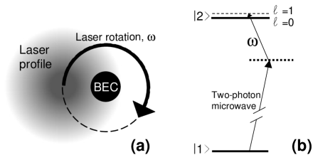
FIG. 14.: (a) A basic schematic illustration of the technique used to create a vortex. An off-resonant laser provides a rotating force on the atoms across the condensate as a microwave drive of detuning $\delta$ is applied. (b) A level diagram showing the microwave transition to very near the $\left|2\right>$ state, and the modulation due to the laser rotation frequency that couples only to the angular momentum $l=1$ state when $\omega\approx\delta$.

(Taken from Ref. [33])

In practice, $\omega\gg\omega_{0}$ and $\delta\gg\Omega$. The first inequality allows the vortex to be generated rapidly. The main problem with a slow drive (when $\omega\approx\omega_{0}$) is that the time scale for coupling to the vortex state is very long, on the order of seconds in a trap with $\omega_{0}=10$ Hz. The weak-coupling limit, given by the second inequality, allows the resonance condition $\omega\approx\delta$ to select energetically the desired state with high fidelity.

Figure 15 shows the results of a numerical integration of Eq. (156) in two dimensions ($\omega_{z}=0$), with the condensate initially in the nonrotating ground state and in the internal state $|1\rangle$ [165]. The coupling drive is turned on at time $t=0$, and is turned off at time $t=t_{s}$ by setting both $\Omega$ and $\rho_{0}$ to zero. The top and the bottom graphs show the fractional population and the angular momentum per atom of the $|2\rangle$ state as a function of time.

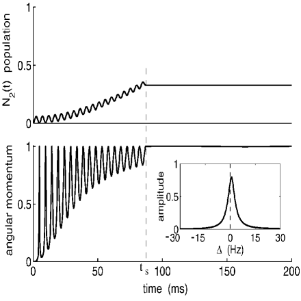
FIG. 15.: Dynamical evolution that can create a vortex. The top graph shows the fractional population of atoms in the $|2\rangle$ internal state. The bottom graph shows the angular momentum of the $|2\rangle$ state, in units of Planck’s constant $\hbar$. The inset shows the amplitude of population transfer to the vortex as a function of the trap rotation frequency $\omega$, with $\Delta=\Omega_{\rm{eff}}-\omega$. The various parameters used in the calculation are: $\omega_{0}=10$ Hz, $\delta=200$ Hz, $\omega=205.4$ Hz, $N=8\times 10^{5}$ atoms, $M$ is the mass of the ⁸⁷Rb atom, for simulations the values of scattering lengths are taken to be $a_{11}=a_{22}=a_{12}=5.5$ nm, and for $t<t_{s}$, $\Omega=50$ Hz and $\rho_{0}=1.7\mu$m. Reprinted by permission from Nature 401, 568, (1999), ©1999 Macmillan Magazines Ltd.

The small-amplitude rapid oscillations on the top graph correspond to the cycling between internal levels at the effective Rabi frequency $\Omega_{{\rm{eff}}}$. The gradual rise of this line reflects coupling from the ground state to the vortex mode caused by the drive $\hat{H}_{1}$ in Eq. (156). Once during each Rabi cycle, the angular momentum approaches unity (bottom graph), and, at that time, the $|2\rangle$ state wave function approaches a pure vortex mode. By turning off the coupling at a precise time $t=t_{s}$ on a given Rabi cycle, the $|2\rangle$ state can be prepared to have unit angular momentum. The maximum possible population transfer to the vortex state using this scheme obeys a Lorentzian response curve as $\omega$ is varied near $\Omega_{{\rm eff}}$, exhibiting a narrow resonance. This situation is shown in the inset of Fig. 15, where $\Delta=\Omega_{{\rm{eff}}}-\omega$.

In an experiment, it is possible put the initial condensate into either the $\left|1\right\rangle$ or $\left|2\right\rangle$ state, and then make a vortex in the $\left|2\right\rangle$ or $\left|1\right\rangle$ state, respectively. The evolution of the vortex can be watched over time scales from milliseconds to seconds. In Ref. [33], the vortex was found to be stable in only one of the two possible configurations corresponding to the vortex in the $|1\rangle$ state, which is the one with the larger scattering length (with the $|2\rangle$ state in the core). The other possibility (the vortex in the $|2\rangle$ state, which is the one with the lowest self-interaction coefficient) produces an instability.

B Stability Theory

We use the following notation for the states: $(1,0)$ for the state with the vortex in $|1\rangle$ and $(0,1)$ for the state with the vortex in $|2\rangle$. In the JILA experiment [33], the number of particles is the same for each component ($N_{1}=N_{2}=N$) but, in general, one could consider any ratio between the populations of the different levels. The scattering lengths for binary collisions depend on the internal hyperfine level of the atom. For ⁸⁷Rb the values of scattering lengths are nearly degenerate and in the proportion $a_{11}:a_{12}:a_{22}=1.00:0.97:0.94$ [171]. Because of the relation $U_{11}>U_{12}>U_{22}$, the experiment is performed in a regime in which the first component separates from the second one. Consequently, a favored configuration has the first component spread over the largest part of the space. Numerical simulations show that in the equal population case, $N_{1}=N_{2}=N$, and for arbitrary nonlinearities, the stationary states $(1,0)$ is stable while the other state $(0,1)$ is unstable.

The origin of the instability of the state $(0,1)$ is purely dynamical [172] and can be understood within the framework of mean-field theories for the double-condensate system without dissipation. Actually, the instability mechanism does not lead to expulsion of the vortex from the condensate, but to periodic transfer of the phase singularity from one species to the other. To study the vortex stability, one can start from a pair of coupled Gross Pitaevskii equations for the condensate wave functions of each species

$$i\hbar\frac{\partial}{\partial t}\Psi_{1}=\left[-\frac{\hbar^{2}\nabla^{2}}{2M}+V_{1}+U_{11}|\Psi_{1}|^{2}+U_{12}|\Psi_{2}|^{2}\right]\Psi_{1},$$ (158)

$$i\hbar\frac{\partial}{\partial t}\Psi_{2}=\left[-\frac{\hbar^{2}\nabla^{2}}{2M}+V_{2}+U_{21}|\Psi_{1}|^{2}+U_{22}|\Psi_{2}|^{2}\right]\Psi_{2},$$ (159)

where $V_{1}$ and $V_{2}$ are trap potentials for the condensate components. These equations are a particular case of Eq. (156) when the drive is turned off ($\hat{H}_{1}$, $\Omega$, $\delta=0$). Equations (158) and (159) conserve the number of particles in each hyperfine level. However, the angular momentum of each component is no longer a conserved quantity, and the topological charge of each species can change through the time evolution. Instead, what is conserved is the total angular momentum of the system

$$L_{z}=i\hbar\int d^{3}r{\Psi}_{1}^{*}\partial_{\phi}\Psi_{1}+i\hbar\int d^{3}r{\Psi}_{2}^{*}\partial_{\phi}\Psi_{2}.$$ (160)

As in the JILA experiments, we assume that both potentials are spherically symmetric and have the form $V_{1}({\bf r})=V_{2}({\bf r})=\frac{1}{2}M\omega_{0}^{2}(r_{\perp}^{2}+z^{2})$. For stationary configurations in which each component has a well-defined value of the angular momentum, the time and angular dependence are factored out

$$\Psi_{i}(r_{\perp},z,\phi)=e^{-i\mu_{i}t/\hbar}e^{iq_{i}\phi}\psi_{i}(r_{\perp},z),$$ (161)

with $i=1,2$. We focus on three particular configurations, which are the lowest energy states with vorticity $(q_{1},q_{2})=(0,0),(1,0),(0,1)$. They correspond to the ground state of the double condensate, and to the single vortex states for the $|1\rangle$ and $|2\rangle$ species, respectively.

Linear stability analysis of the three states gives the following results [172]. For the $(0,0)$ state, the frequencies of all normal modes are positive, as expected for the ground state of the system. Among the normal modes of the $(1,0)$ family, there is a negative eigenvalue, which means that there is a path in the configuration space along which the energy decreases (this is just the analog of the anomalous mode in the one-component system with a vortex). This path belongs to a perturbation that takes the vortex out of the condensate. As in the case of a single-component condensate, however, the lifetime of the vortex state is only limited by the presence of dissipation (without dissipation, the configuration is dynamically stable). Finally, in the $(0,1)$ family, there are normal modes with complex frequencies. The shape of the unstable modes is similar to the energy-decreasing modes of the $(1,0)$ family — that is, they are perturbations that push the vortex out of both clouds. The imaginary part of the eigenvalues implies that vortices with unit charge in $|2\rangle$ are unstable under a generic perturbation of the initial data, whereas those in $|1\rangle$ can be long-lived. This conclusion is consistent with the JILA experiments, where a vortex in the $|2\rangle$ species was found to be unstable [33].

Numerical simulations of the vortex behavior for large perturbations show that the linearly stable state $(1,0)$ is robust and survives under a wide range of perturbations, suffering at most a precession of the vortex core plus changes of the shapes of both components [172]. This behavior arises in both two- and three-dimensional simulations. In contrast, the unstable configuration $(0,1)$ develops a recurrent dynamics. In the first stage, the first component and the vortex oscillate synchronously (the hole in $|2\rangle$ pins the peak of $|1\rangle$). These oscillations grow in amplitude, and the vortex spirals out. Finally the first component develops a tail and later a hole which traps the second component. The hole is a vortex that has been transferred from $|2\rangle$ to $|1\rangle$. Though not completely periodic, this mechanism exhibits some recurrence, and the vortex eventually returns to $|2\rangle$. The preceding behavior persists even for strong perturbations in a two-dimensional condensate. However, for large perturbations of a three-dimensional condensate, the dynamics may lead to a turbulent behavior [172].

In Fig. 16, it is shown how a small initial perturbation makes the phase singularity in $|2\rangle$ spiral out of the system while a phase singularity appears in $|1\rangle$ and occupies the center of the atomic cloud. This dynamics is recurrent.

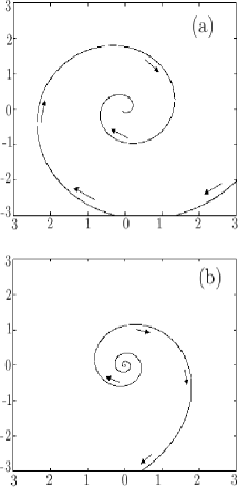
FIG. 16.: Evolution of the position of the phase singularity in the $xy$ plane. Lengths are given in units of the trap characteristic length $d=\sqrt{\hbar/M\omega_{0}}$. (a) Phase singularity in $|1\rangle$, (b) phase singularity in $|2\rangle$.

(Taken from Ref. [173]).

The preceding results are valid for the equal population case, $N_{1}=N_{2}$. For any ratio of the populations $N_{1}/N_{2}$ and any values of the nonlinear coefficients $U_{ij}$, the stability conditions are the following [173]: The configuration $(1,0)$ is stable if

$$\left(\sqrt{\frac{N_{1}}{N_{2}}}-1\right)^{2}>1-\frac{a_{11}}{a_{12}}.$$ (162)

For ⁸⁷Rb, the inequality (162) is always satisfied, which proves that the configuration with a vortex in $|1\rangle$ is always linearly stable, as found in  [33]. Note that the stability properties do not depend on the total number of particles but only on the ratio between the populations.

The stability condition of the configuration $(0,1)$ is

$$\left(\sqrt{\frac{N_{2}}{N_{1}}}-1\right)^{2}>1-\frac{a_{22}}{a_{21}}$$ (163)

This inequality fails for a certain range of $N_{1}/N_{2}$. For the case of ⁸⁷Rb the unstable range is $N_{1}/N_{2}\in[0.73,1.49]$, which means that certain choices of the population imbalance allow stabilization of the vortex in $|2\rangle$. These results predict the possibility of stable vortex states for various multiple-condensate systems [173].

Energetic considerations show that the extra degree of freedom associated with the second component allows a more intricate structure for the free-energy surface. As a result, in a two-component system, it is possible to achieve a local minimum in the free energy at the center of the trap [124]. The presence of such a minimum implies the existence of a region of energetic stability where the vortex cannot escape and might generate a persistent current.

VIII Conclusions and outlook

In this paper, we have provided an introductory description of vortices in trapped Bose condensed gases. The main conclusion of our analysis is that the vortex dynamics in such systems is well described by the time-dependent Gross-Pitaevskii equation (at least for low temperatures). The nonuniform nature of the condensate results in the appearance of anomalous vortex mode(s) with negative frequency and positive norm. Trap rotation shifts the normal-mode frequencies and can stabilize the vortex state. To date, experimental measurements of vortex dynamics and other properties of vortex states are in a good quantitative agreement with theoretical predictions based on solutions of the GP equation. Deviations from the mean-field predictions could arise when the gas parameter $\bar{n}|a|^{3}$ is not very small (semiclassical corrections to the mean-field approximation were calculated in [174] ) or from “mesoscopic” effects associated with the finite systems. However, there is no experimental evidence for these effects so far.

We have been able to cover only part of the existing literature on vortices in trapped condensates. Among important issues that we have not discussed are: different methods of vortices generation and detection, kinetics of vortex nucleation and decay, vortices in BECs with attractive interactions and in Fermi condensates, other defects in BECs (solitons, instantons, vortex solitons, skyrmions, wave-function and spin monopoles).

In the case of superfluid helium, vortex nucleation is associated with pinning of vortex lines at the walls of the container. Trapped condensates have no rough surfaces, and the nucleation process of quantized vorticity has a different origin [175, 116, 176]. An important question in vortex nucleation is the role of the thermal component and transverse anisotropy of magnetic traps [177, 178].

The literature of the past few years contains many different proposals for the creation of vortices in trapped BECs, although we considered only a few of them in this review. To illustrate the diversity of different methods, let us cite some other schemes. An experimental setup for vortex creation by Berry’s phase induced Bose-Einstein condensation is proposed by Olshanii and Naraschewski [179]. A related vortex-production scheme employing the Aharonov-Casher effect is discussed by Petrosyan and You [180]. Other proposals suggest the creation of the vortex state by opto-mechanical stirring [167]; by a rotating force [181]; by an adiabatic population transfer of a condensate from the ground to the excited Bose-condensed state via a Raman transition induced by laser light [166, 168, 165]; the accidental generation of vortices in a quench [182, 183] or in self-interference measurements [169].

A possible way to create rotating states from a trapped ground-state BEC by using light-induced forces is proposed by Marzling and Zhang [184]. They show that the dipole potential induced by four traveling-wave laser beams with an appropriate configuration in space, phase and frequency can be used to realize such a system. Vortex states can be trapped in an evaporative cooling process if the evaporation length is less than the size of the thermally excited state [185, 183]. In order to nucleate vortices, the trapped gas can be rotated at temperatures above the BEC transition. Recently, it has been suggested that vorticity could be imprinted by imaging a BEC through an absorption plate [186]. The method consists of passing a far-off-resonant laser pulse through an absorption plate with an azimuthally dependent absorption coefficient, imaging the laser beam onto a BEC, and thus creating the corresponding nondissipative Stark-shift potential and condensate phase shift. A vortex ring may be formed by translating one condensate through another one [187] (this process is analogous to ring nucleation by moving ions in superfluid ⁴He [188]), or by three-dimensional soliton decay [189, 190]. Recently the JILA group generated vortex rings by the decay of dark solitons through the snake instability [191].

Many different proposals for the detection of vortices in BECs have been mentioned in literature. Some of them are used in current experiments. The spatial size of the vortex core in the TF regime is too small to be observed; for visualizing the vortex state, it was suggested to switch off the trap and let the cloud expand ballistically [82]. After expansion, the size of the vortex core is magnified by approximately the same factor as the size of expanding condensate [70, 192], so that the core becomes observable. Also the vortex state can be detected by the splitting of the collective condensate modes in axisymmetric traps [62, 111, 115] or by looking at the phase slip in the interference fringes produced by two expanding condensates [167, 70]. Dobrek et al. [186] proposed an interference method to detect vortices by coherently pushing part of the condensate with optically induced Bragg scattering. A detection scheme that reveals the existence of vortex states in a cylindrically symmetric trap is discussed by Goldstein, Wright and Meystre [193]. This scheme relies on the measurement of the second-order correlation function of the Schrödinger field and yields directly the topological charge of the vortex state.

Also one can detect the vortex state by observing the off-resonance absorption image of the rotational cloud [166]. For a vortex state one should expect a bright “hole” in the image which accounts for the vortex core in the density distribution. Another possibility is to observe the Doppler frequency shift due to the quantized circular motion of the atoms [166], or by scattering fast atoms in a pure momentum state off a trapped atomic cloud [194].

Another question that has recently attracted significant theoretical and experimental interest is the dynamics and stability of dark solitons and vortex solitons in trapped condensates. Solitary waves (kinks) have been studied in many physical contexts [195] and exist in different physical, chemical and biological systems [196]. Recent theoretical studies discuss the dynamics and stability of dark solitons [197, 198, 199, 200, 201] (the range of parameters where the solitons are dynamically stable has been determined in [99, 101], while the theory of dissipative dynamics of a kink at finite temperature condensates has been developed in [202]), as well as suggestions for their creation  [168, 203, 186]. Recently dark solitons inside a condensate were generated by a phase-imprinting method [204, 205]. Unlike vortices, dark solitons are not topologically stable. At finite temperature, they exhibit thermodynamic and dynamic (small-amplitude) instabilities. The interaction of the soliton with the thermal cloud causes dissipation that accelerates the soliton. There is an interesting analogy between solitons and relativistic particles, in which the soliton velocity and speed of sound correspond to the particle velocity and speed of light in vacuum [202]. However, the kinematic mass of the soliton decreases when its velocity increases. This behavior is opposite to the case of relativistic particle, where the kinematic mass increases with velocity, and an infinite force is required to accelerate the particle beyond the velocity of light. In contrast to the particle, the soliton can reach the velocity of sound. An interesting problem is to create a soliton and a vortex simultaneously (this object is known as vortex soliton). The vortex soliton has a topological charge and therefore could be stable.

Another challenging perspective for future experiments is the creation of vortex-like states in optically confined BECs. By relaxing the condition of spin polarization imposed by magnetic trapping, this new method of confinement permits the study of diverse textures that can be formed by the spinor order parameter, like those in superfluid ³He-A [20]. Also optical traps allow strong variation of the scattering length via Feshbach resonances, which provides new possibilities for manipulating the condensate states.

Among other challenging problems, one should mention measurements of vortex normal modes at higher temperatures, which could establish the connection between the Bogoliubov approximation and self-consistent mean field theories. Also, it would be interesting to observe vortex dissipation and damping of vortex normal modes.

- [1] M. H. Anderson, J. R. Ensher, M. H. Matthews, C. E. Wieman, and E. A. Cornell, Science 269, 198 (1995).
- [2] C. C. Bradley, C. A. Sackett, J. J. Tollett, and R. G. Hulet, Phys. Rev. Lett. 75, 1687 (1995).
- [3] K. B. Davis, M.-O. Mewes, M. R. Andrews, N. J. van Druten, D. S. Durfee, D. M. Kurn, and W. Ketterle, Phys. Rev. Lett. 75, 3969 (1995).
- [4] A. Griffin, Excitations in Bose-Condensed Liquid (Cambridge University Press, New York, 1993).
- [5] P. Sokol, in Bose-Einstein Condensation, edited by A. Griffin, D. W. Snoke and S. Stringari, (Cambridge University Press, Cambridge, 1995), p.51.
- [6] T.-L. Ho and V. B. Shenoy, Phys. Rev. Lett. 77, 2595 (1996).
- [7] E. M. Lifshitz and L. P. Pitaevskii, Statistical Physics, Part 2, 3rd edition (Pergamon, Oxford, 1980), Sec. 29.
- [8] D. R. Tilley and J. Tilley, Superfluidity and Superconductivity (Adam Hilger Ltd., Bristol, 1986), 2nd ed.
- [9] W. F. Vinen, Superconductivity, edited by R. D. Parks (Marcel Dekker, New York, 1969) Chap. 20.
- [10] L. Onsager, Nuovo Cimento 6, Suppl. 2, 249 and 281 (1949).
- [11] R. P. Feynman, in Progress in Low Temperature Physics, edited by C. J. Gorter (North-Holland, Amsterdam, 1955), Vol. I, p. 17
- [12] W. F. Vinen, Proc. R. Soc. London A 260, 218 (1961).
- [13] E. J. Yarmchuck, M. J. V. Gordon, and R. E. Packard, Phys. Rev. Lett. 43, 214 (1979).
- [14] R. J. Donnelly, Quantized Vortices in Helium II (Cambridge University Press, Cambridge, U. K., 1991).
- [15] F. V. Dolzhanskii, V. A. Krymov, and D. Yu. Manin, Usp. Fiz. Nauk 160, 1 (1990) [Sov. Phys. Usp. 33, 495 (1990)].
- [16] D. M. Sedrakyan and K. M. Shakhabasyan, Usp. Fiz. Nauk 161, 3 (1991) [Sov. Phys. Usp. 34, 555 (1991)].
- [17] G. N. Fowler, S. Raha, and R. M. Weiner, Phys. Rev. C 31, 1515 (1985).
- [18] D. Vollhardt and P. Wölfle, The Superfluid Phases of Helium 3 (Taylor & Francis, London, 1990), Ch. 7.
- [19] The term “skyrmion” symbolizes an image of extended baryon, being regarded as a topological soliton, made up of bosons but possessing fermion features. Such a soliton was considered by Skyrme in his model which describes the low-energy limit of quantum chromodynamics. For a review of the Skyrme model and strong interactions see V. G. Makhan’kov, Yu. P. Rybakov, and V. I. Sanyuk, Usp. Fiz. Nauk 162, 1 (1992) [Sov. Phys. Usp. 35, 55 (1992)].
- [20] T.-L. Ho, Phys. Rev. Lett. 81, 742 (1998); e-print cond-mat/9803231.
- [21] J. J. García-Ripoll, J. I. Cirac, J. Anglin, V. M. Perez-García, and P. Zoller, Phys. Rev. A. 61, 053609 (2000).
- [22] M. Krusius, P. J. Hakonen, and J. T. Simola, in Proceeding of the 17th International Conference on Low Temperatures Physics, Physica Ser. B+C 126, 22 (1984).
- [23] G. E. Volovik, in Proceeding of the 17th International Conference on Low Temperatures Physics, Physica Ser. B+C 126, 34 (1984). For a review of superfluid properties of 3He- and 3He- see also G. E. Volovik, Usp. Fiz. Nauk 143, 73 (1984) [Sov. Phys. Usp. 27, 363 (1984)] and V. P. Mineev, Usp. Fiz. Nauk 139, 303 (1983) [Sov. Phys. Usp. 26, 160 (1983)].
- [24] A. L. Fetter, in Progress in Low Temperature Physics, Vol. X, edited by D. F. Brewer (North-Holland, Amsterdam, 1986), p. 1.
- [25] M. M. Salomaa and G. E. Volovik, Rev. Mod. Phys. 59, 533 (1987).
- [26] P. G. Saffman, Vortex Dynamics (Cambridge University Press, Cambridge, 1997).
- [27] C. A. Jones and P. H. Roberts, J. Phys. A: Math. Gen. 15, 2599 (1982).
- [28] T. Frisch, Y. Pomeau, and S. Rica, Phys. Rev. Lett. 69, 1644 (1992).
- [29] J. Koplik and H. Levine, Phys. Rev. Lett. 71, 1375 (1993).
- [30] J. Koplik and H. Levine, Phys. Rev. Lett. 76, 4745 (1996).
- [31] F. Dalfovo, S. Giorgini, L. P. Pitaevskii, and S. Stringari, Rev. Mod. Phys. 71, 463 (1999).
- [32] G. Baym and C. J. Pethick, Phys. Rev. Lett. 76, 6 (1996).
- [33] M. R. Matthews, B. P. Anderson, P. C. Haljan, D. S. Hall, C. E. Wieman, and E. A. Cornell, Phys. Rev. Lett. 83, 2498 (1999).
- [34] K. W. Madison, F. Chevy, W. Wohlleben, and J. Dalibard, Phys. Rev. Lett. 84, 806 (2000).
- [35] K. W. Madison, F. Chevy, W. Wohlleben, and J. Dalibard, J. Mod. Optics 47, 2715 (2000).
- [36] F. Chevy, K. W. Madison, and J. Dalibard, Phys. Rev. Lett. 85, 2223 (2000).
- [37] B. P. Anderson, P. C. Haljan, C. E. Wieman, and E. A. Cornell, Phys. Rev. Lett. 85, 2857 (2000).
- [38] N. N. Bogoliubov, J. Phys. (USSR) 11, 23 (1947).
- [39] E. P. Gross, Nuovo Cimento 20, 454 (1961).
- [40] E. P. Gross, J. Math. Phys. 4, 195 (1963).
- [41] L. P. Pitaevskii, Zh. Eksp. Teor. Fiz. 40, 646 (1961) [Sov. Phys. JETP 13, 451 (1961)].
- [42] A. L. Fetter and J. D. Walecka, Quantum Theory of Many Particle Systems (McGraw-Hill, New York, 1971), Sec. 35.
- [43] A. L. Fetter, in Bose-Einstein Condensation in Atomic Gases, Proceedings of the International School of Physics “Enrico Fermi,” edited by M. Inguscio, S. Stringari, and C. E. Wieman (IOS Press, Amsterdam, 1999), p. 201.
- [44] E. Tiesinga, C. W. Williams, P. S. Julienne, K. M. Jones, P. D. Lett, and W. D. Phillips, J. Res. Natl. Inst. Stand. Technol. 101, 505 (1996).
- [45] H. M. J. M. Boesten, C. C. Tsai, J. R. Gardner, D. N. Heinzen, and B. J. Verhaar, Phys. Rev. A 55, 636 (1997).
- [46] E. R. I. Abraham, W. I. McAlexander, C. A. Sackett, and R. G. Hulet, Phys. Rev. Lett. 74, 1315 (1995).
- [47] F. Dalfovo and S. Stringari, Phys. Rev. A 53, 2477 (1996).
- [48] S. L. Cornish, N. R. Claussen, J. L. Roberts, E. A. Cornell, and C. E. Wieman, Phys. Rev. Lett. 85, 1795 (2000).
- [49] L. D. Landau and E. M. Lifshitz, Fluid Mechanics, 2nd edition, (Pergamon, London, 1987), Chap. I.
- [50] A. L. Fetter and J. D. Walecka, Theoretical Mechanics of Particles and Continua (McGraw-Hill, New York, 1980), Sec. 48.
- [51] V. L. Ginzburg and L. P. Pitaevskii, Zh. Eksp. Teor. Fiz. 34, 1240 (1958) [Sov. Phys. JETP 7, 858 (1958)].
- [52] A. L. Fetter, Phys. Rev. 138, A429 (1965).
- [53] A. L. Fetter, Phys. Rev. 151, 100 (1966).
- [54] F. Lund, Phys. Lett. A 159, 245 (1991).
- [55] S. Rica and E. Tirapegui, Phys. Rev. Lett. 64, 878 (1990).
- [56] S. Rica and E. Tirapegui, Physica D 61, 246 (1992).
- [57] S. Stringari, Phys. Rev. Lett. 77, 2360 (1996).
- [58] M. Tinkham, Introduction to Superconductivity (McGraw-Hill, New York, 1975), Chap. 5.
- [59] V. V. Konotop and V. M. Pérez-García, Phys. Rev. A 62, 033610 (2000).
- [60] N. K. Wilkin, and J. M. F. Gunn, Phys. Rev. Lett. 84, 6 (2000).
- [61] G. Moore and N. Read, Nucl. Phys. B 360, 362 (1991).
- [62] S. Sinha, Phys. Rev. A 55, 4325 (1997).
- [63] D. S. Rokhsar, Phys. Rev. Lett. 79, 2164 (1997).
- [64] A. A. Svidzinsky and A. L. Fetter, Physica B 284-288, 21 (2000).
- [65] E. M. Lifshitz and L. P. Pitaevskii, Statistical Physics, Part 1, 3rd edition (Pergamon, Oxford, 1980), Sec. 26.
- [66] N. K. Wilkin, J. M. F. Gunn, and R. A. Smith, Phys. Rev. Lett. 80, 2265 (1998).
- [67] D. A. Butts and D. S. Rokhsar, Nature 397, 327 (1999).
- [68] M. Linn and A. L. Fetter, Phys. Rev. A 60, 4910 (1999).
- [69] E. Lundh, C. J. Pethick, and H. Smith, Phys. Rev. A 55, 2126 (1997).
- [70] Y. Castin and R. Dum, Eur. Phys. J. D 7, 399 (1999).
- [71] H. Shi and W. Zheng, Phys. Rev. A 55, 2930 (1997).
- [72] S. Stringari, Phys. Rev. Lett. 82, 4371 (1999).
- [73] H. Lamb, Hydrodynamics, 6th edition (Dover, New York, 1945), pp. 86-88.
- [74] A. L. Fetter, J. Low Temp. Phys. 16, 533 (1974).
- [75] D. L. Feder, C. W. Clark, and B. I. Schneider, Phys. Rev. Lett. 82, 4956 (1999).
- [76] D. L. Feder, C. W. Clark, and B. I. Schneider, Phys. Rev. A 61, 011601(R) (2000).
- [77] K. DeConde and R. E. Packard, Phys. Rev. Lett. 35, 732 (1975).
- [78] A. A. Svidzinsky and A. L. Fetter, Phys. Rev. Lett. 84, 5919 (2000).
- [79] F. Dalfovo, L. P. Pitaevskii, and S. Stringari, Phys. Rev. A 54, 4213 (1996)
- [80] F. Dalfovo, S. Giorgini, M. Guilleumas, L. P. Pitaevskii, and S. Stringari, Phys. Rev. A 56, 3840 (1997).
- [81] T. Isoshima and K. Machida, Phys. Rev. A 60, 3313 (1999).
- [82] E. Lundh, C. J. Pethick, and H. Smith, Phys. Rev. A 58, 4816 (1998).
- [83] D. L. Feder, A. A. Svidzinsky, A. L. Fetter, and C. W. Clark, Phys. Rev. Lett 86, 564 (2001).
- [84] E. L. Andronikashvili, Yu. G. Mamaladze, S. G. Matinyan, and D. S. Tsakadze, Usp. Fiz. Nauk 73, 3 (1961) [Sov. Phys. Usp. 4, 1 (1961)].
- [85] G. A. Williams and R. E. Packard, Phys. Rev. Lett. 33, 280 (1974).
- [86] E. J. Yarmchuk and R. E. Packard, J. Low Temp. Phys. 46, 479 (1982).
- [87] V. K. Tkachenko, Zh. Eksp. Teor. Fiz. 49, 1875 (1966) [Sov. Phys. JETP 22, 1282 (1966)].
- [88] G. B. Hess, Phys. Rev. 161, 189 (1967).
- [89] D. Stauffer and A. L. Fetter, Phys. Rev. 168, 156 (1968).
- [90] L. J. Campbell and R. M. Ziff, Phys. Rev. B 20, 1886 (1979).
- [91] G. M. Kavoulakis, B. Mottelson, and C. J. Pethick, Phys. Rev. A 62, 063605 (2000).
- [92] P. C. Haljan, B. P. Anderson, I. Coddington, and E. A. Cornell, e-print cond-mat/0012320.
- [93] Y. A. Nepomnyashchii, Teor. Mat. Fiz. 20, 399 (1974).
- [94] W. B. Colson and A. L. Fetter, J. Low Temp. Phys. 33, 231 (1978).
- [95] A. L. Fetter, Ann. Phys. (N.Y.) 70, 67 (1972).
- [96] A. L. Fetter, Phys. Rev. A 53, 4245 (1996).
- [97] H. Pu, C. K. Law, J. H. Eberly, and N. P. Bigelow, Phys. Rev. A 59, 1533 (1999).
- [98] I. Aranson and V. Steinberg, Phys. Rev. B 53, 75 (1996).
- [99] A. E. Muryshev, H. B. van Linden van den Heuvell, and G. V. Shlyapnikov, Phys. Rev. A 60, R2665 (1999).
- [100] P. O. Fedichev, A. E. Muryshev, and G. V. Shlyapnikov, Phys. Rev. A 60, 3220 (1999).
- [101] D. L. Feder, M. S. Pindzola, L. A. Collins, B. I. Schneider, and C. W. Clark, Phys. Rev. A 62, 053606 (2000).
- [102] J. J. García-Ripoll and V. M. Peréz-García, Phys. Rev. A 60, 4864 (1999).
- [103] L. J. Garay, J. R. Anglin, J. I. Cirac, and P. Zoller, Phys. Rev. A 63, 023611 (2001).
- [104] M. Edwards, R. J. Dodd, C. W. Clark, and K. Burnett, J. Res. Natl. Inst. Stand. Technol. 101, 553 (1996).
- [105] L. D. Landau, J. Phys. (USSR) 5, 71 (1941).
- [106] Reference [7], Secs. 22 and 23.
- [107] Reference [49], Chap. IX.
- [108] L. D. Landau, E. M. Lifshitz, and L. P. Pitaevskii, Electrodynamics of Continuous Media, 2nd edition (Pergamon, Oxford, 1984), Sec. 115.
- [109] J. D. Jackson, Classical Electrodynamics, 3rd edition (Wiley, New York, 1998), Sec. 13.4.
- [110] A. L. Fetter and D. Rokhsar, Phys. Rev. A 57, 1191 (1998).
- [111] A. A. Svidzinsky and A. L. Fetter, Phys. Rev. A 58, 3168 (1998).
- [112] R. J. Dodd, K. Burnett, M. Edwards, and C. W. Clark, Phys. Rev. A 56, 587 (1997).
- [113] A. L. Fetter, J. Low Temp. Phys. 113, 198 (1998).
- [114] A. A. Svidzinsky and A. L. Fetter, unpublished (see e-print: cond-mat/9811348).
- [115] F. Zambelli and S. Stringari, Phys. Rev. Lett. 81, 1754 (1998).
- [116] J. J. García-Ripoll and V. M. Peréz-García, e-print: cond-mat/0006368.
- [117] A. A. Svidzinsky and A. L. Fetter, Phys. Rev. A 62, 063617 (2000).
- [118] V. M. Pérez-García, H. Michinel, J. I. Cirac, M. Lewenstein, and P. Zoller, Phys. Rev. Lett. 77, 5320 (1996).
- [119] V. M. Pérez-García, H. Michinel, J. I. Cirac, M. Lewenstein, and P. Zoller, Phys. Rev. A 56, 1424 (1997).
- [120] M. Linn and A. L. Fetter, Phys. Rev. A 61, 063603 (2000).
- [121] R. E. Packard and T. M. Sanders, Jr., Phys. Rev. A 6, 799 (1972).
- [122] B. Jackson, J. F. McCann, and C. S. Adams, Phys. Rev. A 61, 013604 (2000).
- [123] E. Lundh and P. Ao, Phys. Rev. A 61, 063612 (2000).
- [124] S. A. McGee and M. J. Holland, e-print: cond-mat/0007143.
- [125] D. Feder, private communication.
- [126] L. M. Pismen and J. Rubinstein, Physica D 47, 353 (1991).
- [127] B. Y. Rubinstein and L. M. Pismen, Physics D 78, 1 (1994).
- [128] L. M. Pismen, Vortices in Nonlinear Fields (Clarendon Press, Oxford, 1999), Secs. 2.2 and 5.2.
- [129] C. F. Barenghi, Phys. Rev. A 54, 5445 (1996).
- [130] Reference [50], Sec. 40.
- [131] L. D. Landau and E. M. Lifshitz, Mechanics (Pergamon, Oxford, 1960), Secs. 36 and 37.
- [132] D. Kleppner and R. Kolenkow, An Introduction to Mechanics (McGraw-Hill, New York, 1973), Sec. 7.3.
- [133] Reference [50], Sec. 28.
- [134] A. Griffin, Phys. Rev. B 53, 9341 (1996).
- [135] P. O. Fedichev and G. V. Shlyapnikov, Phys. Rev. A 58, 3146 (1998).
- [136] S. T. Beliaev, Sov. Phys. JETP 34, 299 (1958).
- [137] L. Pitaevskii and S. Stringari, Phys. Rev. Lett. 81, 4541 (1998).
- [138] T. Isoshima and K. Machida, J. Phys. Soc. Jpn. 66, 3502 (1997).
- [139] D. A. W. Hutchinson, R. J. Dodd, and K. Burnett, Phys. Rev. Lett. 81, 2198 (1998).
- [140] N. P. Proukakis, S. A. Morgan, S. Choi, and K. Burnett, Phys. Rev. A 58, 2435 (1998).
- [141] S. M. M. Virtanen, T. P. Simula, and M. M. Salomaa, poster, workshop on rotating Bose condensates, Trento, Italy, June 11-13, 2000; to appear in Phys. Rev. Lett.
- [142] T. Isoshima and K. Machida, Phys. Rev. A 59, 2203 (1999).
- [143] P. O. Fedichev and G. V. Shlyapnikov, Phys. Rev. A 60, R1779 (1999).
- [144] E. B. Sonin, Phys. Rev. B 55, 485 (1997).
- [145] Yu. N. Ovchinnikov and I. M. Sigal, Nonlinearity 11, 1295 (1998).
- [146] D. P. Arovas, and J. A. Freire, Phys. Rev. B 55 1068 (1997).
- [147] V. Ambegaokar, B. I. Halperin, D. R. Nelson, and E. D. Siggia, Phys. Rev. B 21 1806 (1980).
- [148] A. P. Chikkatur, A. Görlitz, D. M. Stamper-Kurn, S. Inouye, S. Gupta, and W. Ketterle, Phys. Rev. Lett. 85, 483 (2000).
- [149] C. Raman, M. Köhl, R. Onofrio, D. S. Durfee, C. E. Kuklewicz, Z. Hadzibabic, and W. Ketterle, Phys. Rev. Lett. 83, 2502 (1999).
- [150] R. Onofrio, C. Raman, J. M. Vogels, J. R. Abo-Shaeer, A. P. Chikkatur, and W. Ketterle, Phys. Rev. Lett. 85, 2228 (2000).
- [151] C. Huepe and M. E. Brachet, C. R. Acad. Sci. Paris 325, 195 (1997).
- [152] B. Jackson, J. F. McCann, and C. S. Adams, Phys. Rev. Lett. 80, 3903 (1998).
- [153] C. Nore, C. Huepe, and M. E. Brachet, Phys. Rev. Lett. 84
- [154] T. Winiecki, J. F. McCann, and C. S. Adams, Phys. Rev. Lett. 82, 5186 (1999).
- [155] B. M. Caradoc-Davies, R. J. Ballagh, and K. Burnett, Phys. Rev. Lett. 83, 895 (1999).
- [156] S. Burkhart, M. Bernard, O. Avenel, and E. Varoquaux, Phys. Rev. Lett. 72, 380 (1994).
- [157] C. J. Myatt, E. A. Burt, R. W. Ghrist, E. A. Cornell, and C. E. Wieman, Phys. Rev. Lett. 78, 586 (1997).
- [158] D. M. Stamper-Kurn, M. R. Andrews, A. P. Chikkatur, S. Inouye, H.-J. Miesner, J. Stenger, and W. Ketterle, Phys. Rev. Lett. 80, 2027 (1998).
- [159] J. Stenger, S. Inouye, D. M. Stamper-Kurn, H.-J. Miesner, A. K. Chikkatur, and W. Ketterle, Nature (London) 396, 345 (1998).
- [160] J. C. Wheatley, in Progress in Low Temperature Physics, Vol. VI, edited by C. J. Gorter (North-Holland, Amsterdam, 1970), p. 77.
- [161] N. D. Mermin and T.-L. Ho, Phys. Rev. Lett. 36, 594 (1976).
- [162] See, for example, Reference [18], Chap. 17, p. 210.
- [163] S.-K. Yip, Phys. Rev. Lett. 83, 4677 (1999).
- [164] T. Ohmi and K. Machida, J. Phys. Soc. Jpn. 67, 1822 (1998).
- [165] J. E. Williams and M. J. Holland, Nature 401, 568 (1999).
- [166] K.-P. Marzlin, W. Zhang, and E. W. Wright, Phys. Rev. Lett. 79, 4728 (1997).
- [167] E. L. Bolda and D. F. Walls, Phys. Lett. A 246, 32 (1998).
- [168] R. Dum, J. I. Cirac, M. Lewenstein, and P. Zoller, Phys. Rev. Lett. 80, 2972 (1998).
- [169] J. Ruostekoski, Phys. Rev. A 61, 041603 (2000).
- [170] J. Williams, R. Walser, J. Cooper, E. A. Cornell, and M. Holland, Phys. Rev. A 61, 033612 (2000).
- [171] D. S. Hall, M. R. Matthews, J. R. Ensher, C. E. Wieman, and E. A. Cornell, Phys. Rev. Lett. 81, 1539 (1998).
- [172] J. J. García-Ripoll and V. M. Pérez-García, Phys. Rev. Lett. 84, 4264 (2000).
- [173] V. M. Pérez-García and J. J. García-Ripoll, Phys. Rev. A 62, 033601 (2000).
- [174] J. Andersen and E. Braaten, Phys. Rev. A 60, 2330 (1999).
- [175] J. P. Martikainen, K. A. Suominen, and A. Sanpera, e-print: cond-mat/0005136.
- [176] F. Dalfovo and S. Stringari, Phys. Rev. A 63, 011601 (2001).
- [177] A. Recati, F. Zambelli, and S. Stringari, Phys. Rev. Lett. 86, 377 (2001).
- [178] K. W. Madison, F. Chevy, V. Bretin, and J. Dalibard, e-print: cond-mat/0101051.
- [179] M. Olshanii, and M. Naraschewski, e-print: cond-mat/9811314.
- [180] K. G. Petrosyan and L. You, Phys. Rev. A 59, 639 (1999).
- [181] K.-P. Marzlin and W. Zhang, Phys. Rev. A 57, 4761 (1998).
- [182] J. R. Anglin and W. H. Zurek, Phys. Rev. Lett. 83, 1707 (1999).
- [183] P. D. Drummond and J. F. Corney, Phys. Rev. A 60, R2661 (1999).
- [184] K.-P. Marzlin and W. Zhang, Phys. Rev. A 57, 3801 (1998).
- [185] R. J. Marshall, G. H. C. New, K. Burnett, and S. Choi, Phys. Rev. A 59, 2085 (1999).
- [186] L. Dobrek, M. Gajda, M. Lewenstein, K. Sengstock, G. Birkl, and W. Ertmer, Phys. Rev. A 60, R3381 (1999).
- [187] B. Jackson, J. F. McCann, and C. S. Adams, Phys. Rev. A 60, 4882 (1999).
- [188] G. W. Rayfield and F. Reif, Phys. Rev. 136, 1194 (1964).
- [189] C. A. Jones, S. J. Putterman, and P. H. Roberts, J. Phys. A 19, 2991 (1986).
- [190] C. Josserand and Y. Pomeau, Europhys. Lett. 30, 43 (1995).
- [191] B. P. Anderson, P. C. Haljan, C. A. Regal, D. L. Feder, L. A. Collins, C. W. Clark, E. A. Cornell, e-print: cond-mat/0012444.
- [192] F. Dalfovo and M. Modugno, Phys. Rev. A 61, 023605 (2000).
- [193] E. V. Goldstein, E. M. Wright, and P. Meystre, Phys. Rev. A 58, 576 (1998).
- [194] A. B. Kuklov and B. V. Svistunov, Phys. Rev. A 60, R769 (1999).
- [195] R. Rajaraman, Solitons and Instantons (North-Holland, Amsterdam, 1987).
- [196] B. S. Kerner and V. V. Osipov, Usp. Fiz. Nauk 157, 201 (1989) [Sov. Phys. Usp. 32, 101 (1989)].
- [197] W. Zhang, D. F. Walls, and B. C. Sanders, Phys. Rev. Lett. 72, 60 (1994).
- [198] W. P. Reinhardt and C. W. Clark, J. Phys. B 30, L785 (1997).
- [199] S. A. Morgan, R. J. Ballagh, and K. Burnett, Phys. Rev. A 55, 4338 (1997).
- [200] A. D. Jackson, G. M. Kavoulakis, and C. J. Pethick, Phys. Rev. A 58, 2417 (1998).
- [201] D. Margetis, J. Math. Phys. 40, 5522 (1999).
- [202] P. O. Fedichev, A. E. Muryshev, and G. V. Shlyapnikov, Phys. Rev. A 60, 3220 (1999).
- [203] T. F. Scott, R. J. Ballagh, and K. Burnett, J. Phys. B 31, L329 (1998).
- [204] S. Burger, K. Bongs, S. Dettmer, W. Ertmer, K. Sengstock, A. Sanpera, G. V. Shlyapnikov, and M. Lewenstein, Phys. Rev. Lett. 83, 5198 (1999).
- [205] J. Denschlag, J. E. Simsarian, D. L. Feder, Charles W. Clark, L. A. Collins, J. Cubizolles, L. Deng, E. W. Hagley, K. Helmerson, W. P. Reinhardt, S. L. Rolston, B. I. Schneider, W. D. Phillips, Science 287, 97 (2000).