Clustering in a model with repulsive long-range interactions

Abstract

A striking clustering phenomenon in the antiferromagnetic Hamiltonian Mean-Field model has been previously reported. The numerically observed bicluster formation and stabilization is here fully explained by a non linear analysis of the Vlasov equation.

and

1 Introduction

The Hamiltonian Mean Field model (HMF) [1] has attracted much attention in the recent years as a toy model to study the dynamics of systems with long-range interactions, and its relation to thermodynamics [2]. Its Hamiltonian describes an assembly of fully coupled rotors

$$H=\sum_{i=1}^{N}\frac{p_{i}^{2}}{2}+\frac{c}{2N}\sum_{i,j=1}^{N}\cos(\theta_{i}-\theta_{j})$$ (1)

where $\theta_{i}$ is the angle of the rotor and $p_{i}$ its conjugate angular momentum. Since we will use periodic boundary conditions, this model can be alternatively viewed as representing particles moving on a circle, whose positions are given by the $\theta_{i}$. In this paper we consider the case in which the interaction among the particles is repulsive (corresponding to the antiferromagnetic rotor model), i.e. $c=1$. As first noticed in Ref. [1], this model has a very interesting dynamical behaviour. In contrast with statistical mechanics predictions, a bicluster forms at low energy for a special but wide class of initial conditions (see Fig. 1 for the corresponding density profile). For any initial spatial distribution of particles, the bicluster develops in time from a homogeneous density state as shown in Fig. 2, if the initial velocity dispersion is weak. This clustering and the unexpected dependence on initial conditions were studied in Ref. [3] but the phenomenon remained unexplained. In this paper we give an explanation of the incipient formation of the bicluster based on a fully analytical study of the low temperature solutions of the Vlasov equation. We also show some connections of this problem with active transport in hydrodynamics [4], and the formation of caustics in the flow of the Burgers equation.

Figure 1: Equilibrium density distribution for $N=10^{4}$ particles and the energy per particle $U\simeq 10^{-5}$. The diamonds are numerical data and the solid curve is a fit taken from [3].

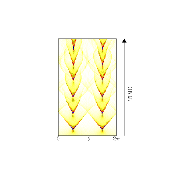
Figure 2: Bicluster formation. Time is running in the upward direction and the system is started with a constant particle density: the darker the grey, the bigger the density. One notices the very quick concentration of particles, followed by the repeated appearance of “chevrons”, shrinking as time increases.

2 Hydrodynamical description at zero temperature

We begin by performing first the thermodynamic limit, $N\to\infty$, i.e. by writing the Vlasov equation of Hamiltonian (1). Calling $f(\theta,p,t)$ the one particle distribution function, we have

$$\frac{\partial f}{\partial t}+p\frac{\partial f}{\partial\theta}-\frac{1}{2\pi}\int_{-\infty}^{+\infty}du\int_{0}^{2\pi}d\alpha\ f(\alpha,u,t)\sin(\theta-\alpha)\frac{\partial f}{\partial p}=0$$ (2)

We can define a density $\rho$, a velocity field $v$, and a velocity dispersion $\sigma^{2}$ as follows

$$\rho(\theta,t) = \int_{-\infty}^{+\infty}f(\theta,p,t)dp$$

$$\rho(\theta,t)v(\theta,t) = \int_{-\infty}^{+\infty}pf(\theta,p,t)dp$$

$$\sigma^{2}(\theta,t) = \frac{1}{\rho}\int_{-\infty}^{+\infty}p^{2}f(\theta,p,t)dp-v^{2}(\theta,t)~{}.$$

The numerics shows that the bicluster appears when the velocity dispersion is small. We will then neglect $\sigma^{2}$, which corresponds to a zero temperature approximation. A straightforward calculation reduces now the Vlasov equation to the hydrodynamical equations for $\rho$ and $v$

$$\frac{\partial\rho}{\partial t}+\frac{\partial(\rho v)}{\partial\theta} = 0$$ (3)

$$\frac{\partial v}{\partial t}+v\frac{\partial v}{\partial\theta} = \frac{1}{2\pi}\int_{0}^{2\pi}d\alpha\ \rho(\alpha,t)\sin(\theta-\alpha)~{}.$$ (4)

The first equation accounts for the mass conservation and the second one is the Euler equation without pressure term. Hence, the dynamics of the model at zero temperature is mapped onto this active scalar advection problem [4], which we will now solve approximately at short time. We first linearize the above equations, assuming the velocities are small and the density almost uniform. We are left with

$$\frac{\partial\rho}{\partial t}+\frac{\partial v}{\partial\theta}=0$$

$$\frac{\partial v}{\partial t}=\frac{1}{2\pi}\int_{0}^{2\pi}\rho(\alpha,t)\sin(\theta-\alpha)~{},$$

a system that we can solve by means of Fourier series. Assuming a vanishing initial velocity field, we get

$$\rho(\theta,t)=\sqrt{2}v_{m}\cos\theta\cos\omega t$$

$$v(\theta,t)=v_{m}\sin\theta\sin\omega t~{},$$ (5)

where $\omega=\sqrt{2}/2$ is the plasma frequency. The amplitude $v_{m}$ and the longer wavelength components of $\rho$ in (5) are fixed by the initial condition. This linear analysis describes very well the short time evolution of the system, a few plasma periods. Of course this is not sufficient to explain the bicluster formation and it is useful to carry out the non linear analysis: this analysis relies on the existence of two time-scales in the system.

• The inverse of the plasma frequency, which is intrinsic and of order one.

• The timescale connected to the energy of the system of order $1/\sqrt{U}$.

If the energy is sufficiently small, the two time-scales are very different, and it becomes possible to use averaging methods. We introduce the long time-scale $\tau=\epsilon t$, with $\epsilon=v_{m}/\sqrt{2}$ ($v_{m}$ is directly related to the energy per particle $U$), and we write

$$v(\theta,t)=v_{m}\sin\theta\sin\omega t+\epsilon u(\theta,\tau)$$ (6)

We have also to estimate the force in the non linear regime. As a zeroth order approximation, we use the expression given by the linear analysis. Since the force depends only on the first Fourier component of the density (due to the special form of the Hamiltonian), this approximation amounts to suppose that the sinusoidal behaviour of this first component, found in the linear regime (5), remains valid in the non-linear regime. This may appear very crude, but the numerics shows on the contrary that it is a quite good approximation. This fact deserves a comment. Exploiting an analogy with the plasmas studied in Ref. [5], our system may be seen as a bulk of particles interacting with waves sustained by the bulk itself. Here, there is one wave, materialized by the small oscillations in the density and the velocity field found in the linear approximation. Since at small energy the phase velocity of the wave (of order one like the plasma frequency) is much higher than the velocities of the bulk particles (of order $\sqrt{U}$), the wave has almost no interactions with these particles, and stands forever. This gives a qualitative explanation of the fact that the linear approximation for the force in Euler equation (4) is so accurate. We introduce now expression (6) into equation (4). The terms of first order in $\epsilon$ on the l.h.s. cancel the force in the r.h.s.. The second order terms gives

$$\frac{\partial u}{\partial\tau}+u\frac{\partial u}{\partial\theta}+2\sin\theta\cos\theta\sin^{2}\omega t+\left(\sin\theta\frac{\partial u}{\partial\theta}+u\cos\theta\right)\sqrt{2}\sin\omega t=0.$$ (7)

Averaging over the short time scale, we get

$$\frac{\partial u}{\partial\tau}+u\frac{\partial u}{\partial\theta}=-\frac{1}{2}\sin 2\theta\quad.$$ (8)

This is a spatially forced Burgers equation without viscosity which describes the motion of fluid particles in a potential given by $V(\theta)=1/4\,\cos 2\theta$. The double well shape of this potential is responsible for the bicluster formation: particles will tend to spend more time in the bottom of the wells. This equation may be solved using the method of characteristics, which presents a great advantage: the characteristics are the Lagrangian trajectories of the Euler equation, so that they are an approximation to the particles trajectories of the real Hamiltonian system. Since the characteristic equation is nothing but the equation of a pendulum

$$\frac{d^{2}\theta}{d\tau^{2}}+\frac{1}{2}\sin 2\theta=0~{},$$ (9)

the Hamiltonian trajectories of the particles can be approximated by pendulum trajectories (see Fig. 3).

We can also explain now the periodic recurrence and the shape of the “chevrons” (Fig. 2): they are zones of infinite density corresponding to the envelopes of the characteristics, so called caustics. Their approximate equation is

$$\theta\propto\frac{\left(t-(2n-1)t_{s}\right)^{3/2}}{\sqrt{n}}$$ (10)

                 

                          

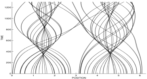
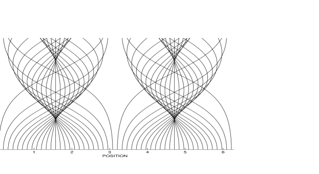
Figure 3: Comparison between real trajectories of the particles (upper figure), and characteristics of equation (8) (lower figure). One can see the two first appearances of the “chevrons”. Two phenomena are not captured by the characteristics: the small and fast oscillations of the real trajectories which have been averaged out, and the presence of untrapped particles, close to the saddle-points of the effective $\cos 2\theta$ potential.

where $n$ is the number counting successive “chevron” appearences in time; the comparison with the numerics is drawn on Fig. 4. The $1/\sqrt{n}$ factor accounts for the shrinking of the “chevrons”. Similar caustics are encountered in astrophysics, to explain the large scale structure of the universe: clusters and super clusters of galaxies are believed to be reminiscent of three dimensional caustics arising from the evolution of an initially slightly inhomogeneous plasma [6].

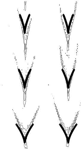
Figure 4: Evolution of density for short times (level curves). The analytical formula for the “chevrons” (10) is superimposed (bold curves). $U\simeq 10^{-4}$ without adjustable parameter.

3 Conclusions

The surprising formation and stabilization of a bicluster in the HMF model [1] is now understood. The small collective oscillations of the bulk of particles create an effective double-well potential, in which the particles evolve. This may be viewed as a nice example of active transport of the density field [4], which can be studied analytically. Lastly, we get an insight on the striking influence of initial conditions: when the initial thermal agitation is too strong, the description of the system by density and velocity fields breaks down. A peculiar behaviour of the trajectories evolving from initial conditions with a small velocity dispersion may be a somewhat general phenomenon for systems with long range interactions; indeed such features have been very recently observed for a self-gravitating system in 1D [7].

References

- [1] M. Antoni and S. Ruffo, Phys. Rev. E 52 (1995) 2361.
- [2] V. Latora, A. Rapisarda and S. Ruffo, Physica D 131 (1999) 38.
- [3] T. Dauxois, S. Ruffo and P. C. W. Holdsworth, Eur. Phys. J. B 16 (2000) 659.
- [4] D. del-Castillo-Negrete, Phys. Lett. A 241 (1998) 99; Physics of Plasmas 5 (1998) 3886; Physica A 280 (2000) 10.
- [5] M. Antoni, Y. Elskens and D. Escande, Physics of Plasmas 5 (1998) 841.
- [6] S.F. Shandarin and Ya.B. Zeldovich, Rev. Mod. Phys. 61 (1989) 185; M. Vergassola, B. Dubrulle, U. Frisch and A. Noullez, Astronomy and Astrophysics 289 (1994) 325.
- [7] H. Koyama and T. Konishi, astro-ph/0010030.