Hysteresis and Avalanches in the Random Anisotropy Ising Model

Abstract

The behaviour of the Random Anisotropy Ising model at $T=0$ under local relaxation dynamics is studied. The model includes a dominant short-range ferromagnetic interaction and assumes an infinite anisotropy at each site along local anisotropy axes which are randomly aligned. As a consequence, some of the effective interactions become antiferromagnetic-like and frustration appears. Two different random distributions of anisotropy axes have been studied. Both are characterized by a parameter that allows control of the degree of disorder in the system. By using numerical simulations we analyze the hysteresis loop properties and characterize the statistical distribution of avalanches occuring during the metastable evolution of the system driven by an external field. A disorder-induced critical point is found in which the hysteresis loop changes from displaying a typical ferromagnetic magnetization jump (large avalanche spanning a macroscopic fraction of the system) to a rather smooth loop exhibiting only tiny avalanches. The critical point is characterized by a set of critical exponents, which are consistent with the universal values proposed from the study of other simpler models.

I INTRODUCTION

Hysteresis occurs in field-driven systems showing history dependence of the corresponding response [1]. Disorder is acknowledged to be a crucial ingredient in determining hysteresis properties, especially in the so-called rate-independent limit. In this case, system properties do no exhibit explicit time dependence. For this to occur, two conditions must be satisfied; (i) thermal fluctuations need to be irrelevant (athermal character) and (ii) field driving rates must be small enough. Ideally, this corresponds to the zero-temperature quasi-static limit. Within this framework, disordered systems can be viewed as described by a multidimensional energy landscape containing many local metastable states separated by large energy barriers. If thermal fluctuations are not operative, these energy barriers can only be overcome by modifying the external field which tilts the energy landscape. The system evolution thus proceeds through jumps from one metastable state to another metastable state and therefore, the field-response shows a discontinuous and apparent stochastic character. In magnetic systems, this jerky magnetization response corresponds to the so-called Barkhausen noise[2]. Moreover, similar behaviour has been reported in many different systems, including martensitic systems [3], superconducting films [4] and capillary condensation systems [5] among others. All these systems exhibit, as a common feature, a field-driven first-order phase transition influenced by disorder. Actually, hysteresis has its origin in this first-order transition and the characteristics of the hysteresis loops depend on both the kind and amount of disorder [6]. With these ideas in mind, different versions of lattice spin models with disorder have been proposed as simple models incorporating the essential physics of these systems. This includes, among other more complicated models, the Random Field (RFIM) [7], the Random Bond (RBIM) [8] and the Site-Diluted (SDIM) [9, 10] Ising models. Such models, with appropriate dynamics, show rate-independent hysteresis and associated Barkhausen noise when sweeping the field at very low temperature. It is also found that the system becomes magnetically softer when the amount of disorder is increased. This is characterized by a change of the hysteresis loops from sharp to smooth. At the same time, the distribution of sizes and durations of Barkhausen signals is also modified [8]. The striking feature is the existence of a specific amount of disorder at which these distributions become critical (power law behaviour). Therefore, the change from sharp to smooth hysteresis loops can be interpreted as a disorder-induced phase transition, as has recently been found experimentally from the study of Co/CoO films [11]. The possible relationship of this phase transition (involving metastable states) with a change of the ground state (equilibrium) of the system is still an open question. A number of recent results point, however, in this direction [10, 12].

In magnetic materials, a physically relevant source of disorder arises from the randomness of the magnetocrystalline anisotropy. This paper is aimed at analysing the intrinsic zero-temperature hysteresis and avalanche properties in systems with such disorder. Actually, the random uniaxial single-site anisotropy Heisenberg model has been considered to be a suitable model to describe magnetic properties of amorphous alloys [13]. At mesoscales, this model can also be used, as a reasonable approximation, to describe granular materials, alloys with precipitates, polycrystalline systems etc…, where grains form single magnetic domains, and changes of magnetization can take place only by rotation of the local magnetization vector. The model was first introduced and studied in the mean field approximation by Harris et al. [14]. Further investigations suggested that in 3$d$, the stable low-temperature phase is a spin glass phase, even in the limit of strong anisotropy. In this limit, the spins are forced to be aligned along the anisotropy axis and therefore, the model reduces to a Random Anisotropy Ising model (RAIM) [15]. This is the model that will be considered in the present study.

To our knowledge, the RAIM has not been studied very much within the above metastable evolution framework, although it is a good candidate to display a disorder induced phase transition [16]. Moreover, it has been argued from symmetry grounds that it should belong to the same universality class as the RFIM [17]. An interesting feature of this model regards the fact that comparison with experiments may be considered as being more realistic than for other more idealized models such as the RFIM or the RBIM. However, modification, in a controlled way, of the amount of disorder in real systems is not always easy to do. For polycrystalline alloys changing the distribution of anisotropy axes is, in principle, possible by impressing an orientation texture by application of a severe cold work process or by means of a heat treatment (recrystallization) [18]. In the case of magnetostrictive amorphous ribbons, anisotropy can be controlled by an external applied stress [19, 20, 21]. The effect of such external stress is to decrease the amount of disorder by inducing a longitudinal anisotropy.

The paper is organized as follows. In the next section we introduce the model and the details of the numerical simulation procedure. In section III we present the results, which include the description of the hysteresis loops, the Barkhausen avalanches, and critical phenomena. Finally in section IV we discuss the results and draw conclusions.

II Modelling

A Hamiltonian

We consider a 3d cubic lattice with spins ${\vec{S}}_{i}$ and local anisotropy axes ${\hat{n}}_{i}$ defined at each site ($i=1,...,N=L^{3})$. Each unitary vector ${\hat{n}}_{i}$ is determined by a pair of spherical polar coordinates $(\theta_{i},\phi_{i})$. Note that since such unitary vectors define a direction in space, the angles are limited to the ranges $0<\phi_{i}<2\pi$ and $0<\theta_{i}<\pi/2$. The axis directions are random and independently distributed according to a generic density probability distribution $f(\theta,\phi)$ which is normalized, i.e.:

$$\int_{0}^{2\pi}d\phi\int_{0}^{\frac{\pi}{2}}f(\theta,\phi)\sin\theta d\theta=1.$$ (1)

The general Hamiltonian of the system can be written as:

$${\cal H}=-\sum_{\langle ij\rangle}^{\frac{z}{2}N}J{\vec{S}}_{i}{\vec{S}}_{j}-\sum_{i=1}^{N}{\vec{H}}{\vec{S}}_{i}-D\sum_{i=1}^{N}\left({\hat{n}}_{i}{\vec{S}}_{i}\right)^{2}-K\sum_{ij}^{N(N-1)}3\frac{(\vec{S}_{j}\vec{r}_{ij})(\vec{S}_{i}\vec{r}_{ij})}{r_{ij}^{5}}-\frac{\vec{S}_{i}\vec{S}_{j}}{r_{ij}^{3}},$$ (2)

where the first term with $J>0$ accounts for the ferromagnetic exchange energy, which is short range and is assumed to extend only to nearest-neigbour pairs ($z=6$ is the coordination number of the cubic lattice). The second term (Zeeman energy) stands for the interaction with an external applied field $\vec{H}$. The third term is the anisotropy energy. Finally, the last term corresponds to the long-range dipolar interactions that extend to all pairs $i,j$ of the lattice. The vector $\vec{r}_{ij}$ is the vector joining sites $i$ and $j$.

In the infinite anisotropy limit ($D>>1$), the spins $\vec{S}_{i}$ are constrained to lie on the $\hat{n}_{i}$ directions and therefore satisfy:

$$\vec{S}_{i}={\hat{n}}_{i}S_{i},$$ (3)

where $S_{i}$ is now an Ising spin variable taking values $\pm 1$. Under such conditions the Hamiltonian of the system can be written as:

$${\cal H}=-J\sum_{\langle ij\rangle}^{\frac{z}{2}N}S_{i}S_{j}\hat{n}_{i}\hat{n}_{j}-\sum_{i}^{N}S_{i}\hat{n}_{i}\vec{H}-DN-K\sum_{ij}^{N(N-1)}S_{i}S_{j}\frac{3(\hat{n}_{j}\hat{r}_{ij})(\hat{n}_{i}\hat{r}_{ij})-(\hat{n}_{i}\hat{n}_{j})}{r_{ij}^{3}}.$$ (4)

The dipolar term represents, in lattice models, a convenient way to describe the magnetostatic energy of the system. Note that it changes from being pure ferromagnetic for a pair of interacting spins with ${\hat{n}}_{i}={\hat{n}}_{j}={\hat{r}}_{ij}$ to pure antiferromagnetic when ${\hat{n}}_{i}={\hat{n}}_{j}\perp{\hat{r}}_{ij}$. The exact treatment of this term in numerical simulations is difficult since the introduction of a cut-off in the interaction range can induce non-physical effects [22]. This term has been recently considered within the context of athermal hysteresis studies in the case of perfectly aligned anisotropy axes [23, 24]. Its main effect on the hysteresis loop is to produce a rather large nucleation jump at the beginning of the demagnetization process. As regards its influence on the properties of the avalanche distributions, it has been argued [25] that its effect is to cause mean-field behaviour. Most of the results in the present work correspond to a situation with rather large randomness. Such randomness and independence of the orientation of the anisotropy axes at two different sites $i$ and $j$ is expected to weaken the importance of the dipolar term. Therefore, we have not considered it in the present work. The Hamiltonian with $K=0$ reads:

$${\cal H}=-\sum_{\langle ij\rangle}^{\frac{z}{2}N}J_{ij}S_{i}S_{j}-H\sum_{i}^{N}g_{i}S_{i},$$ (5)

where the first term is a random bond term with $J_{ij}=J\hat{n}_{i}\hat{n}_{j}$ and the second term describes the random coupling to the external magnetic field (random g-factor) with $g_{i}=\cos\theta_{i}$. The constant term $DN$ in Eq. (4) has been omitted, since it represents only a shift in the energy of the system. Moreover, without loss of generality we will take $J=1$ as the unit of energy.

In the present work we will consider that the external field $\vec{H}$ keeps its direction fixed along the $z$ axis so that only its magnitude $H$ can change. Thus the $g_{i}$ are constant once the initial distribution of anisotropy axis has been quenched (notice that rotation of $\vec{H}$ with fixed modulus could also be considered).

Finally, it should be remarked that the second term in Eq. (5) acts, for each value of $H$, as a random field term. This equivalence, nevertheless, only applies for equilibrium studies. The metastable evolution (hysteresis loops and sequence of avalanches) of such a random g-factor model cannot, a priori, be expected to be equivalent to that of a RFIM.

B Modelling of disorder

As mentioned in the introduction, in real systems such as polycrystalline alloys, the distribution of anisotropy axis is very much dependent on details of the sample preparation. Here we are interested in controlling the amount of disorder in the system by controlling the distribution of angles $f(\theta,\phi)$. We have considered two simplified models, which represent perturbations of the two extreme cases of a fully aligned anisotropy axis and a completely random distribution;

• Model A

  Uniform density within a cone $0<\theta<\theta_{0}$:

  $$f(\theta,\phi)=\frac{1}{2\pi\left(1-\cos{\theta_{0}}\right)}\;h\left[\theta_{0}-\theta\right],$$ (6)

  where $h[x]$ is the Heaviside step function. Note that for $\theta_{0}=0$ the axes are fully aligned in the $z$ direction, while for $\theta_{0}=\pi/2$ the axes are isotropically distributed. The amount of disorder in the system increases with increasing $\theta_{0}$.

• Model B

  First-order correction to the isotropic distribution:

  $$f(\theta,\phi)=(1-\epsilon)\frac{1}{2\pi}+\epsilon\frac{3}{2\pi}\cos^{2}\theta.$$ (7)

  In this case the parameter $\epsilon$ ranges within $-\frac{1}{2}\leq\epsilon\leq 1$ to ensure that $f(\theta,\phi)$ is positive. For $\epsilon>0$ the distribution displays a peak at $\theta=0$, which flattens as $\epsilon$ goes to zero. Thus, in this case, the amount of disorder increases with decreasing $\epsilon$. For $\epsilon=0$ this distribution is uniform and reduces to model A with $\theta_{0}=\pi/2$. When $\epsilon<0$ the distribution shows a maximum at $\theta=\pi/2$, which corresponds to a tendency for the anisotropy axes to lie isotropically on a flat disk perpendicular to the external applied field. Thus, strictly speaking when $\epsilon$ decreases in the $\epsilon<0$ region the anisotropy axes orders again, but perpendicular to the external field. This increases both frustration and competing interactions.

Figures 1 and 2 show a number of examples of the anisotropy axis distribution corresponding to models A and B respectively. The polar plot in the first column corresponds to a particular sample of 1000 anisotropy axes numerically generated according to $f(\theta,\phi)$. The polar angle in these plots represents $\phi$ while the radius represents $\sin\theta$. Note that, with this representation, a uniform distribution of anisotropy axes corresponds to a uniform distribution of points on the circle of unit radius. For each example we show the corresponding distribution of exchange interactions $J_{ij}=\hat{n}_{i}\hat{n}_{j}$. Moreover if the anisotropy axes are restricted to $\theta<\pi/4$, the corresponding exchange interactions are all ferromagnetic $J_{ij}>0$. In contrast, if $\theta>\pi/4$ in the case of some anisotropy axes then the systems contains a fraction of antiferromagnetic bonds.

C Dynamics

Regarding the dynamics of the system, two different situations have been discussed in the literature [25, 26]. The first case corresponds to the dynamics of an interface or domain wall propagating in a disordered media [26, 27]. Actually, domain wall motion is the predominant magnetization process in the approximately constant permeability region of the hysteresis loops [28], and therefore such dynamics is adequate for studies of the linear region of the magnetization curve. The second approach is the so-called field-driven nucleation proposed by Sethna and co-workers [7]. In this case nucleation and growth are treated simultaneously. While in the former case only spins located at the propagating interface can flip, in the latter, any spin of the system can turn when such a flip becomes energetically favourable. This second approach seems more convenient for the study of the full hysteresis loops, in particular in systems with strong local anisotropy and a lack of well-defined domain structure

The details of the dynamics used for the numerical simulations are the following; under slow changes of the external magnetic field, the system follows deterministic dynamics corresponding to local energy relaxation. Due to this local character, the evolution of the system will, in general, not follow an equilibrium path, but rather will evolve through metastable states. Actually, different configurations of spins may correspond to the same value of the external field. Such different configurations are found depending on history conditions.

When studying the full hysteresis loop, the starting point is $H=\infty$ (or $H=-\infty$) which corresponds to the unique stable configuration with all $S_{i}=1$ (or $S_{i}=-1$). We proceed by decreasing (or increasing) the field and compute, from (5), the change of energy $(\Delta{\cal H})_{i}$ associated with the independent reversal of any spin $S_{i}$. This change can be written as

$$(\Delta{\cal H})_{i}=2F_{i}S_{i},$$ (8)

where the local field $F_{i}$ acting on lattice site $i$ is given by;

$$F_{i}=\sum_{n.n.}J_{ij}S_{j}+H\cos\,\theta_{i}.$$ (9)

The metastable states correspond to those configurations of spins for which $\Delta{\cal H}_{i}>0\;\;\forall i$. When for a certain value of $H$ one of the spins become unstable ($(\Delta{\cal H})_{i}=0$), we keep $H$ constant and flip that spin. This can unstabilize some neighbouring spins (for which $(\Delta{\cal H})_{i}<0$) which will be simultaneously flipped (synchronous dynamics). This is the origin of an avalanche. Due to the fact that $\cos\theta_{i}>0$, when decreasing (increasing) the field, the first spin that triggers an avalanche can never yield an increase (decrease) of magnetization. However, such inverse magnetization reversals, may occur during the avalanche. The procedure continues with $H$ constant until all the spins become stable again. This is the end of the avalanche. The external field is then decreased (increased) until a new spin becomes unstable. Notice that the fact that the field remains constant during the avalanche is the crucial condition for rate-independent hysteresis [1]. It is worth noting that in our numerical simulations we have not observed neverending avalanches which may, in general, occur when using this dynamics in systems with antiferromagnetic bonds. Although we cannot provide a rigorous proof for their absence, we suspect that such pathological situations only occur for very special values of the random fields and bonds which have vanishingly small probability when the angles are distributed continuously. The hysteresis loops are obtained by measuring, as a function of $H$, the total magnetization $M$ in the $z$-direction defined as;

$$M=\sum_{i=1}^{N}S_{i}\cos{\theta_{i}}.$$ (10)

Avalanches are characterized by their duration and size. The duration $t$ of the avalanche corresponds to the number of avalanche steps in the algorithm described above. The avalanche size can be quantified in two different ways:

• The total change of magnetization $\Delta M$ between the origin and the end of the avalanche;

  $$\Delta M=\left.\sum S_{i}\cos\theta_{i}\right|_{end}-\left.\sum S_{i}\cos\theta_{i}\right|_{origin}.$$ (11)

  Note that the size of the avalanches, measured in such a way, is bounded by twice the saturation magnetization of the system $M_{sat}=\sum_{i=1}^{N}\cos\theta_{i}$.

• The total number of spins flipped during the avalanche. We will denote such a magnitude by $s$. In this case, as opposed to the above definitions, the avalanche size $s$ is not bounded by the system size $L^{3}$ due to the possibility of inverse spin flips.

III Results

In this section we present the main results of the numerical simulations. We have studied 3d systems with periodic boundary conditions and sizes $L=6,10,20$,$30$ and $40$.

A Hysteresis loops

Figures 3 and 4 show examples of the hysteresis loops corresponding to models A and B (system size $L=10$), with different amounts of disorder (controlled by the parameters $\theta_{0}$ and $\epsilon$ as indicated). First of all, it should be mentioned that the loops are symmetrical with respect to changes $H\rightarrow-H$ and $M\rightarrow-M$. This property comes directly from the symmetry of the Hamiltonian (5).

For both models the qualitative morphological changes of the loops when disorder increases are very similar. Figure 5 shows the dependence of the saturation magnetization $M_{sat}$, the remanent magnetization $M_{rem}$, the coercive field $H_{coe}$ and the total dissipation (area within the loop) $W$ on the parameter ($\theta_{0}$ or $\epsilon$) controlling the amount of disorder. In both cases $M_{sat}$, $M_{rem}$, and $W$ decrease with increasing disorder. Notice that $M_{sat}$ can be obtained exactly by integration of $f(\theta,\phi)cos(\theta)$ over all the spatial directions. The most remarkable difference concerns the behaviour of $H_{coe}$. In model A it exhibits a monotonous decrease with increasing disorder. In model B after the initial decrease of $H_{coe}$ with increasing disorder, a minimun is reached; for negative values of $\epsilon$, $H_{coe}$ increases. From these averaged morphological magnitudes apparently no signs of singular behaviour as a function of the amount of disorder is found. The detection of a possible disorder-induced critical point needs a detailed study of avalanches which will be presented in the next subsection.

It is illustrative to show a sequence of snapshots of the system configuration during a demagnetization process. These are shown in Fig. 6 which corresponds to model A with $L=20$ and $\theta_{0}=1.3$. Black indicates the lattice sites with reversed spins $S_{i}=-1$. The simulation starts from saturation (all the $S_{i}=1$) with a very large applied field. The different configurations correspond to the same plane (of the 3d system) for decreasing values of the external field $H=-0.10,-1.10,-1.44,-1.48,-1.49$. During the first stages of the demagnetizing process the main dynamical mechanism is the nucleation of the reverse magnetization phase by flipping isolated spins. In contrast, in the middle of the hysteresis loop the evolution takes place by growth (depinning) of such domains. This occurs by means of large avalanches which produce reversals of large fractions of the system.

Prior to the analysis of such avalanches it is interesting to consider another feature of the hysteresis loops. The analysis of partial cycles enables study of the existence of the so-called return point memory (RPM) property. The mathematical conditions for such a property to occur have been discussed for the RFIM [7], the RBIM [3] and the SDIM [10]. The two RAIM models (A and B) studied in this work do not exhibit such a property, except for those situations in which no effective antiferromagnetic interactions occur. Figure 7 shows an example of internal loops revealing the failure of the RPM property. This is due to the existence of reverse spin flips during the avalanches, and even reverse avalanches that occur for large enough amounts of disorder. It is worth mentioning that such reverse flips represent a small fraction of the total number of flips. For instance, close to the critical amount of disorder (defined below) it represents less than $5\%$.

B Barkhausen avalanches

The statistical analysis of the avalanches is performed by measuring its size $s$ and duration $t$, in a half hysteresis loop. Figure 8 shows the probability $p(s)$ of occurence of an avalanche of size $s$ for model $A$ and increasing values of the amount of disorder $\theta_{0}$. Data, represented in log-log plots correspond to the analysis of $300$ different half-loops with different realizations of the disorder. For small values of $\theta_{0}$, the cycles contain a very large avalanche giving a peak on the right-hand side of the plot and a certain fraction of small avalanches, on the left. This behaviour is called “supercritical”. On the other hand, for large values of $\theta_{0}$ the system behaves “subcritically” showing only small avalanches. For an intermediate value $\theta_{0}^{c}(L=30)=1.44\pm 0.01$, the distribution of avalanches becomes a power-law (“critical”) characterized by an exponent $\tau^{\prime}=2.06\pm 0.05$. The details of the exponent fitting procedure together with the study of the dependence with the finite size of the system will be presented in the next section. Figure 9 shows the avalanche size distribution $p(s)$ for model $B$. In this case critical behaviour is found at $\epsilon^{c}(L=30)\sim 0.2$ with a power-law exponent $\tau^{\prime}=2.10\pm 0.05$

It is interesting to consider the following two remarks concerning such avalanche size distributions. On the one hand, the avalanche analysis could also be performed by characterizing the avalanche size by $\Delta M$, instead of $s$. Figure 10 shows a comparison of the two histograms (number of avalanches versus size) $N(s)$ and $N(\Delta M)$ in the case of model A with $L=20$, $\theta_{0}=1.39$ and averages over $300$ different realizations. The agreement between both histograms is very good. Even in the small avalanche size region both histograms exhibit almost the same behaviour indicating that effects related to the existence of inverse jumps are totally negligible. Therefore, from now on, we will only consider $p(s)$ distributions. (Note that in figure 10 the histogram $N(\Delta M)$ has been constructed by taking bins of size $\Delta M=8$. This is not necessary for $N(s)$ since $s$ is a discret variable. Thus, for the sake of comparison, the histogram $N(\Delta M)$ must be displayed after being divided by a factor $8$).

On the other hand, it should be mentioned that the large avalanches occuring in the supercritical case span the full simulated system at least in one direction. This is illustrated in Fig. 11 which corresponds to the avalanche distribution of model A with size $L=20$ and $\theta_{0}=1.39$. For this amount of disorder the system still behaves slightly supercritically. The three histograms correspond to the distribution of all the avalanches (bottom), the non-spanning avalanches (middle) and the spanning ones (top). The inset shows the histogram of spanning avalanches on a linear scale, revealing the existence of a characteristic size, which increases when disorder decreases and system size increases. Actually, in the thermodynamic limit such spanning avalanches will be infinite, involving a macroscopic fraction of the the system and giving rise to magnetization discontinuities in the hysteresis loop. It is worth noting that in previous studies of the same problem in the RFIM [6] such spanning avalanches were substracted from the histograms for the analysis of the critical behaviour. In the present work we have decided to keep them since, as will be seen, their occurence provides a criteria for locating the critical point.

C Criticality

The power-law behaviour of the avalanche size distributions reveals the existence of criticality in the system. For this reason such transitions related to the change of properties of the hysteresis loop and of the Barkhausen noise distribution when disorder is increased are called disorder-induced critical points. They share many similarities with the classical critical points, but one should never forget that a number of features are different; firstly we are dealing with a history-dependent metastable evolution of the system, i.e. an out-of-equilibrium problem, thus many thermodynamical equations relating critical exponents, may not be valid [29, 30]. At this point it should be mentioned that for the RFIM, for which the exact equilibrium trajectories can be obtained, it has been found numerically that a transition point exists for the same amounts of disorder in equilibrium. [30]. A second remark concerns the fact that we are dealing with a deterministic phenomenon at $T=0$ and thus fluctuations (in the standard sense), do not exist. By studying systems with different realizations of the disorder corresponding to the same probability distribution $f(\theta,\phi)$, one can define average values of any generic property $z$ that we will denote as $\langle z\rangle$. We can also define “fluctuations” as $\langle z^{2}\rangle-\langle z\rangle^{2}$, but the extrapolation of these averages to the thermodynamic limit may hide some mathematical inconsistencies.

The consequences arising from the two remarks above are still not totally understood. For instance, for such disorder-induced critical points it is not clear what the order parameter is. One choice is the system magnetization per site $\langle M/L^{3}\rangle$. Nevertheless, the fact that the system displays hysteresis for both $\theta_{0}<\theta_{0}^{c}$ and $\theta_{0}>\theta_{0}^{c}$ implies that $\langle M/L^{3}\rangle$ does not go to zero at the critical point. For the RFIM, Sethna and coworkers [6] use $\langle M/L^{3}\rangle-\langle M_{c}/L^{3}\rangle$ (where $M_{c}$ is the value of the magnetization at the critical point). Besides the fact that this quantity does not remain equal to zero above the critical point, it adds to the problem of determining $M_{c}$. A second choice, which was originally used for the study of the RBIM [8], is to measure the size $\langle s_{max}\rangle$ of the largest avalanche in the hysteresis loop. Clearly this is a quantitiy that for a finite system is not a suitable order parameter since it never goes to zero. However, for the infinite system, $\langle s_{max}/L^{3}\rangle$ will be zero for any degree of disorder except for those for which an avalanche spanning a macroscopic portion of the system occurs. This leads to the existence of a discontinuity in the hysteresis loop. Thus, in the present paper, we have chosen this quantity as the order parameter.

Figure 12 displays the behaviour of $\langle s_{max}/L^{3}\rangle$ as a function of $\theta_{0}$ for different system sizes. Data corresponds to averages over $50,200,300,500$ and $300$ different realizations of the disorder for $L=40,30,20,10$ and $6$ respectively. The (pseudo-) phase transition for the finite system will correspond to the inflection point of such curves. The exact location of $\theta_{0}^{c}(L)$ can be obtained, for instance, by means of a 4rth-order polynomial fitting of the inflection point or, after a numerical derivative, a 2nd-order polynomial fitting of the maximum. This gives two slightly different estimations of the the critical point. An independent way of locating the phase transition is to measure the duration $t_{max}$ of the longest avalanche in the half hysteresis loop. The average of such a quantity $\langle t_{max}/L\rangle$ is also shown in Fig. 12 as a function of $\theta_{0}$ for different system sizes ($t_{max}$ is normalized by $L$ since this is the minimum number of steps needed in order to cover the full system). This quantity displays a maximum at $\theta_{0}^{c}(L)$ which is also fitted by using a 2nd-order polynomial. Figure 13 shows equivalent data to that of Figure 12 for model B. In this case only systems up to $L=30$ have been studied. The simulation of larger systems in this case is much more time consuming than for model A due to the wider distribution of anisotropy axes.

A fourth method for the location of the critical point results from the quantitative analysis of the avalanche size distribution of Figs. 8 and 9. These distributions correspond to the statistical analysis of all the avalanches occuring in full half-loops for many realizations of disorder. In general they are well fitted by an exponentially corrected power-law probability distribution [16];

$$p(s;\tau^{\prime},\lambda)=\frac{1}{A}s^{-\tau^{\prime}}e^{-\lambda s},$$ (12)

where $A$ is not an extra free parameter but the normalization factor. As mentioned before the avalanche size $s$ takes discrete values and, strictly speaking, is not bounded from above due to the possibility of inverse flips. For the computation of the normalization factor $A$ we have chosen the largest value $s_{max}$ of each set of data, which in all cases has been found to be lower than $L^{3}$. Thus $A$ (which is a function of $\tau^{\prime}$ and $\lambda$) is given by:

$$A(\tau^{\prime},\lambda)=\sum_{s=1}^{s_{max}}s^{-\tau^{\prime}}e^{-\lambda s}.$$ (13)

The fits are performed by the maximum likelihood method, which is independent of any binning process or representation. Examples of the fits are also shown in Fig. 8. As a general comment, it should be mentioned that the fits are very good for the subcritical, critical and slightly supercritical distributions. For the deep supercritical distributions they are not that good due to two different problems; (i) the existence of large avalanches which span an important fraction of the system makes it difficult to have enough statistics and (ii) the fact that the proposed model (Eq. 12) is not well suited to describe the occurence of the peak (with a certain characteristic size) in the large $s$ regions.

For model A the values obtained of $\lambda$ and $\tau^{\prime}$ as a function of $\theta_{0}$ are shown in Fig. 14 for different system sizes ($L=10,20$ and $30$). For small amounts of disorder $\theta_{0}<\theta_{0}^{c}$, one gets $\lambda<0$. For $\theta_{0}>\theta_{0}^{c}$, one gets $\lambda>0$. The estimation of $\theta_{0}^{c}(L)$ can be obtained by interpolating the value of $\theta_{0}$ for which $\lambda(\theta_{0})=0$. This, nevertheless, shows large uncertainites that increase for increasing values of $L$. The same kind of analysis can be performed with the corresponding similar results for model B. They are shown in Fig. 15.

The four estimations above of $\theta_{0}^{c}(L)$ are shown in Fig. 16 as a function of $L^{-1}$. The results exhibit a strong dependence on the size $L$ of the simulated system, as occurs in numerical simulation of standard critical phenomena. As can be seen the four estimations of $\theta_{0}^{c}$ decrease with increasing $L$. Except for the data obtained from the analysis of the distribution of avalanches which shows large error bars, the linear extrapolation to $L\rightarrow\infty$ indicates a compatible common value for $\theta_{0}^{c}(L\rightarrow\infty)$.

The exact treatment of the dependence of the measured quantities with $L$ must be performed within the framework of finite-size scaling. [31].

D Finite-size scaling

According to the standard finite-size scaling hypothesis, as a function of system size $L$, $s_{max}$ and $t_{max}$ behave as:

$$s_{max}(x,L)/L^{3}\sim L^{-\frac{\beta}{\nu}}F_{s}\left(xL^{\frac{1}{\nu}}\right)$$ (14)

$$t_{max}(x,L)\sim L^{\frac{z}{\nu}}F_{t}\left(xL^{\frac{1}{\nu}}\right),$$ (15)

where $x$ is the reduced amount of disorder. For the case of model A, $x=(\theta_{0}-\theta_{0}^{c}(L))/\theta_{0}^{c}(L)$. The functions $F_{s}$ and $F_{t}$ are scaling functions and $\beta$, $z$ and $\nu$ are critical exponents. The different estimations of the critical amounts of disorder $\theta_{0}^{c}(L)$ for the finite system should also scale with $L$ as:

$$\theta_{0}^{c}(L)-\theta_{0}^{c}(\infty)\sim L^{-\frac{1}{\nu}}.$$ (16)

There are different ways to fit the four exponents $\beta$, $\tau^{\prime}$, $z$ and $\nu$ and determine $\theta_{0}^{c}(\infty)$. Since the behaviour of $\theta_{0}^{c}(L)$ is quite linear with $L$ in Fig. 16, this suggests that to a first approximation it is reasonable to take $\nu\sim 1$. This justifies the linear fits shown in Fig. 16. A value consistent with all the extrapolations is $\theta_{0}^{c}(\infty)=1.33\pm 0.03$ (indicated by an arrow on the vertical axis). With this estimation of $\theta_{0}^{c}(\infty)$ we can refine the value of $\nu$ by performing a linear fit to the log-log plot of $\left(\theta_{0}^{c}(L)-\theta_{0}^{c}(\infty)\right)$ vs. $L$. The obtained value is $\nu=1.0\pm 0.1$

Once $\theta_{0}^{c}(\infty)$ and $\nu$ are determined, the exponents $\beta$ and $z$ can be obtained by analyzing the change with $L$ of the height and slope at the inflection point in the curve $s_{max}(\theta_{0},L)$ and the height and curvature at the maximum in $t_{max}(\theta_{0},L)$. From linear fits to log-log plots the following estimations are obtained: $\beta=0.06\pm 0.05$, $-\beta+1/\nu=0.8\pm 0.1$, $z=1.6\pm 0.02$ and $z+2/\nu=3.3\pm 0.2$. Such values are consistent with a final estimation of $\beta=0.1\pm 0.1$ and $z=1.6\pm 0.1$. The goodness of the final set of exponents can be finally tested by plotting the scaling fuctions $F_{t}$ and $F_{s}$, which are shown in Fig. 17. Within a rather good approximation data collapses onto a single curve, which demonstrates the assumed scaling hypothesis.

A similar analysis has been performed for model B. In this case, instead of fitting a new set of exponents we have tried to scale the data in Fig. 13 with the set of exponents obtained above for model A. The resulting scaling functions are shown in Fig. 18. Again a good data collapse is obtained, demostrating the validity of the scaling hypothesis for model B with the same set of critical exponents.

A summary of the exponents found are given in Table I. Values corresponding to other 3d models and mean-field calculations are also presented for comparison. This point will be discussed in section IV.

E Critical field

The avalanche size distributions analyzed in the previous sections, corresponds to the study of the whole hysteresis cycle. Nevertheless, the simulations of the RFIM [7] suggested that it is convenient to analyze such distributions at different points of the hysteresis loop. Strictly, criticality is expected to occur only at a certain value of the field $H^{c}$ (critical field). In this case the power-law distribution of avalanche sizes is characterized by an exponent $\tau$ which for the RFIM takes a value $\tau=1.6\pm 0.06$ and is related to $\tau^{\prime}$ through a certain scaling relation [17].

The study of $p(s)$ at $H_{c}$ is quite difficult since to obtain sufficiently accurate statistics for a given value of $H$ requires a large number of realizations of disorder. Fig. 19 presents such an analysis for model $A$ in the case of a system with $L=20$, $\theta_{0}=1.39$ ($\sim\theta_{0}^{c}(L=20)$) and averages over $300$ realizations. The distributions have been computed by analysing the avalanches occuring in windows of size $\Delta H=0.5$ around the indicated values of the external applied field during the demagnetizing process. The critical distribution occurs for a field at $|H^{c}(L=20)|\sim-1.5$. For values of $H$ significantly larger and smaller, the distributions exhibits an evident exponential damping. In principle, a more quantitative treatment is possible, which consists of fitting the data with the distribution given by Eq. 12 (replacing $\tau^{\prime}$ by $\tau$). Results for $\tau$ and $\lambda$ are shown in Fig.20 as a function of $H$. The figure reveals the existence of a critical region with $\lambda\sim 0$ and $\tau\sim 1.5$. It is worth noting that outside this critical region, the fit of Eq. 12 renders values of $\tau$ well below the critical value. This method of determining $H^{c}$ is very approximate, since the need for large enough statistics requires a large field window that introduces considerable bias.

Finally, it is interesting to compare $H_{coe}$ with the value of the field $H_{s_{max}}$ at which the largest avalanche ($s_{max}$) for a demagnetizing process (from positive $H$ to negative $H$) occurs. Experimentally, in the region of large disorder $H_{s_{max}}$ can be determined by locating the field for which the macroscopic hysteresis loop exhibits maximum slope, i.e. maximum susceptibility. Figure 21 compares $H_{s_{max}}$ and $H_{coe}$ as a function of $\theta_{0}$ for three different system sizes $L=10$, $20$ and $30$. Data corresponds to averages over $1000,300$ and $300$ realizations of disorder respectively. As expected, for low values of disorder both $H_{s_{max}}$ and $H_{coe}$ coincide; the largest avalanche associated with the magnetization reversal crosses the line $M=0$ and, thus, determines $H_{coe}$. In contrast, for large amounts of disorder the largest avalanche in the hysteresis loop occurs for a value of the field more negative than $H_{coe}$. The inset in figure 21 shows the actual distribution of $H_{s_{max}}$ and $H_{coe}$ over different realizations of disorder and $L=10$. Note that both distributions are quite Gaussian and that for large disorder are split in such a way that the distribution of $H_{coe}$ remains rather sharp while the distribution of $H_{s_{max}}$ broadens. Whether or not the coincidence of $H_{coe}$ and $H_{s_{max}}$ determines the critical field is a question that cannot be definitively answered from our results.

IV Discussion

In this section we compare our results with those corresponding to other models and experiments reported in the litterature.

In the present RAIM, hysteresis arises from energy barriers separating metastable states which have their origin in the effective coupling between spins. This effective coupling is modified by changes in the distribution of anisotropy axes, but even in the absence of disorder, (corresponding to the zero-temperature standard Ising model) hysteresis occurs. In magnetism, hysteresis can be interpreted within the framework of the Stoner-Wohlfarth model (SWM)[32]. This model gives an essentially different description of hysteresis than that proposed in this paper. For the SWM, independent single magnetic domains with continuously orientable magnetic moments are considered. These single domains can be identified with the spins in the present model. Hysteresis, in the SWM, arises from energy barriers originating from the competion between uniaxial anisotropy and Zeeman energy. Actually, no hysteresis occurs in the SW model in the infinite anisotropy limit.

The morphological properties of the hysteresis loops depend, as expected, on the specific characteristics of the disorder. It is interesting to compare the results given in Fig. 5 for coercivity and dissipated energy with available experimental results. Experiments carried out on ribbons of high magnetostrictive amorphous alloys under stress [20, 21] are especially interesting. They reveal that the applied stress favours global (long-range) uniaxial anisotropy which manifests itself by a change of the magnetic domain pattern [19]. Consequently, this leads to a change of the shape of the hysteresis loops. At low external stress, a complicated pattern constituted by maze domains results from the effect of quenched-in stresses. As the external stress is increased, a simpler domain pattern appears with few parallel domains in the direction of the external stress. Therefore, it seems reasonable to assume that the effect of the stress is to reduce the randomness of the local anisotropy axes, or in other words to reduce disorder. The main experimental result [21], is that with increasing external stress, $H_{coe}$ initially exhibits a fast decrease down to a certain minimum value, followed by a roughly linear increase at high stresses. Actually, this effect is reproduced by our model B as can be seen in Fig. (5). This could be explained by taking the competition phenomena arising in the $\epsilon<0$ region for model B mentioned in section II B into account. More quantitative comparisons, nevertheless, are not possible since the actual anisotropy axis distribution in ribbons is difficult to compare with our 3d system. As regards $W$, experimentally it is found that it shows a behaviour similar to that of $H_{coe}$ [20], that is, it exhibits a minimum for a certain value of the applied stress. This is not reproduced either by our models A or B, which show simply a monotonous increase when the system becomes more and more ordered. This disagreement could be due to the fact that in the models, $M_{sat}$ depends on the degree of disorder, as a consequence of the strong anisotropy assumption. Experimentally this is not the case and $M_{sat}$ is almost constant for a given sample composition and thus one expects that $W\propto H_{coe}$.

As regards the critical point our results are totally compatible with the universality that has been proposed for similar athermal models. Table I compares the values obtained in the present work for models A and B with those reported in the literature for the 3d Random Field Ising model , 3d Random Bond Ising model and 3d Site-Diluted Ising model. The agreement is very satisfactory confirming universality [6, 33]. Table I also includes the values of the exponents corresponding to mean-field calculations. Clearly, when considering the full set of all the critical exponents, one concludes that the mean-field model does not belong to the same universality class. This is not surprising since the mean-field approximation assumes long-range interactions while the other models are strictly short range. The mean-field exponent values are expected to be found in systems including dipolar interactions [25]. Nevertheless it should be remarked that the exponents $\tau$ and $\tau^{\prime}$ seem to have, within the errors, comparable values for the two universality classes. Therefore, the analysis of the models suggests that the statistical distribution of avalanches shows very close critical exponents, irrespective of the inclusion or not of the dipolar forces.

It is, perhaps, more interesting to compare such theoretical exponents with those found experimentally. The direct comparison of the numerical values should always be taken carefully since, in experiments, avalanche sizes are determined in different ways depending on the specific measurement technique used. Table II summarizes the most significant values of the exponents reported from the experimental study of Barkhausen noise in magnetic systems [35, 36, 37, 38, 39]. We have separated the $\tau$ exponents corresponding to measurements of noise around a certain value of the external field from the $\tau^{\prime}$ exponents corresponding to the analysis of the signal sequence during the full hysteresis loop (or half loop). In both cases, the numerical procedure for obtaining such experimental exponents is similar to that followed for the analysis of the model simulations; it is based on fitting an expression like Eq. (12) to the recorded histograms of avalanche sizes.

A first remark is that the overall situation concerning the possibility for universality in experiments is not as clear as it is for the theoretical models. In our opinion the main problem is to determine whether the analyzed data corresponds to a critical system or not. A second remark is that the values reported in Table II seem to show a certain dependence on heat treatments and other effects influencing the degree of quenched disorder in the system. For instance, in references [35] and [37] it is found that the $\tau^{\prime}$ exponent increases towards a value close to $2.0$ when the degree of order in the sample is increased by annealing and/or magnetic field cooling. Furthermore the distribution of avalanche sizes in Fe-Co-B alloys (characterized by an exponent $\tau=1.27$ [39] ) were found to change from subcritical towards critical (the cutoff, equivalent to our $\lambda^{-1}$, increases) when the applied tensile stress is increased [21]. In agreement with these results, the $\tau^{\prime}$ exponents in our simulations show a clear increase when the degree of disorder is decreased as can be seen in Figs. 14 and 15. Moreover, our results also suggest that provided that the measurements are performed in the subcritical region, the estimated value of $\tau^{\prime}$ will remain close to the critical value. This could explain why the values of $\tau^{\prime}$ in Table II are quite similar to those found for the models. Actually, the possible existence of a large critical region has also been suggested for the RFIM [6] and for the Site Diluted Random Field Ising model (RFIM with vacancies) [9]. For this last model it has even been proposed that true criticality extends over a broad region of parameters controlling disorder.

A third remark concerns certain procedures used for the estimation of $\tau$ and $\tau^{\prime}$. For instance, for the determination of $\tau^{\prime}$, in some cases saturation is not reached in the studied hysteresis loops. This means that the distributions correspond, in fact, to an internal loop. True saturation requires very high fields which can be not experimentally accessible. At present, it is not clear what the consequences on the measured $\tau^{\prime}$ exponent will be. For the determination of $\tau$, the experiments are carried out with an external field constrained around the coercive field. Our simulations suggest that this may introduce a bias in the estimated exponents. First, if the amount of disorder is greater than the critical amount of disorder, the field at which the largest avalanche takes place and the coercive field do not coincide, as can be seen in Fig. 21. Moreover, even in the case that the disorder is close to the critical value, a deviation in the tuning of the external field would lead to lower values of $\tau$ compared to those expected at $H=H^{c}$, as can be seen in Fig. 20. This may provide an explanation for some of the low values of $\tau$ reported recently [39].

V Summary and conclusion

In this paper we have studied rate-independent hysteresis properties of a Random Anisotropy reticular model. We have considered the infinite uniaxial anisotropy limit and we have neglected any effects of dipolar interactions. In this limit the model reduces to the Random Anisotropy Ising Model which can be viewed as a combination of a Random Bond Ising Model with random couplings (g-factors) to the external magnetic field. This model seems rather appropriate to realistically describe amorphous and polycrystalline magnetic materials. Disorder is introduced in the system through the spatial random distribution of anisotropy axis. Two different distributions, in which disorder is controlled by a single parameter ($\theta_{0}$ and $\epsilon$), have been considered. Extensive numerical simulations of the model have been performed by means of a deterministic algorithm consisting in of synchronous local relaxation dynamics. The morphological properties of the hysteresis loops have been obtained. They depend on the specific distribution of disorder but do not show any singular behaviour when $\theta_{0}$ or $\epsilon$ are varied. Qualitative agreement with some available experimental data has been found. We expect that by choosing a suitable phenomenological distribution of disorder such morphological properties could be better reproduced.

Besides, we have focused on the analysis of the Barkhausen avalanches generated during the metastable evolution. The statistical distribution of such avalanches shows a critical behaviour for a certain amount of disorder ($\theta_{0}^{c}\simeq 1.33\pm 0.03$ and $\epsilon^{c}\sim 0.2$). From a finite-size scaling analysis of different simulated properties we have obtained the critical exponents characterizing the disorder-induced critical point. The most important conclusion is that the present model falls in the same universality class of the athermal 3d RFIM.

We have also analyzed the different available experimental values of such critical exponents characterizing the distribution of Barkhausen signals. Data is scarce and refer to different exponents ($\tau$ and $\tau^{\prime}$). Although there are some discrepancies, the comparison indicates that the experimental systems may fall into the same universality class. However, results suggest that it is necessary to tune the disorder in the systems with adequate thermomechanical treatments so that the system behaves critically. Although a systematic control of the amount of disorder is experimentally difficult, the analysis of our model indicates the best conditions for such measurements and data analysis; (i) disregarding additional experimental problems [40], it is more reliable to measure $\tau^{\prime}$ (full hysteresis loop analysis) instead of $\tau$ in order to avoid problems related to the determination of the critical field $H_{c}$; (ii) although the samples exhibit an exponentially damped power-law distribution (subcritical), the $\tau^{\prime}$ exponents obtained by fitting Eq. 12 render good estimations of the exponents at criticality. Therefore, measurements in the subcritical region are preferable to measurements in the supercritical region.

Model	$\beta$	$\tau^{\prime}$	$\tau$	$z$	$\nu$
3d-RAIM (model A)	$0.1\pm 0.1$	$2.06\pm 0.05$		$1.6\pm 0.1$	$1.0\pm 0.1$
3d-RAIM (model B)	$0.1^{*}$	$2.10\pm 0.05$		$1.6^{*}$	$1.0^{*}$
3d-RFIM [17]	$0.035\pm 0.028$	$2.03\pm 0.03$	$1.6\pm 0.06$		$1.41\pm 0.17$
3d-RBIM [33]	$0.0\pm 0.1$	$2.0\pm 0.2$		$1.6\pm 0.1$	$1.06\pm 0.1$
3d-SDIM [34]		$1.9\pm 0.2$
Mean Field [17]	$1/2$	$2$	$3/2$		$1/2$

TABLE I.: Critical exponents from numerical simulations in this work and in the literature. The values with an asterisk (^∗) have been obtained from model A data and were checked for scaling the data of model B.

Material	Heat treatments	$\tau^{\prime}$	$\tau$	Observ.	Ref.
$81\%$Ni-Fe	$1h$ at $240^{o}C$	$1.73$			[35]
	$1h$ at $460^{o}C$	$2.1$
VITROVAC 6025-X (metal-glass)			$1.77$	small internal loops	[36]
Metglass 2605S-2	as cast	$1.85$		$\tau^{\prime}$ calculated from scaling relations and other measured exponents	[37]
	annealed at $400^{o}C$ and field cooled ($25^{o}C/min$, $120Oe$)	2.0
Perminvar 30$\%$Fe 45$\%$Ni 25$\%$Co	Annealed $1h$, $1000^{o}C$ $24h$ $450^{o}C$		$1.33$		[38]
Fe-Si 7.8 wt%	Annealed $950^{o}C$		$1.5\pm 0.05$	Polycrystalline	[39]
Fe-Si 6.5 wt%	Annealed $1200^{o}C$
	Annealed $1050^{o}C$
Fe21 Co64 B15 Fe64 Co21 B15	as cast		$1.27\pm 0.03$	Amorphous under stress

TABLE II.: Experimental values of the critical exponents $\tau$ and $\tau^{\prime}$

FIG. 1.: Examples of the anisotropy axis distributions of model A for different values of the parameter $\theta_{0}$. The first column corresponds to the polar representation described in the text and the second column to the distributions of random bonds (in arbitrary units).

FIG. 2.: Examples of the anisotropy axis distributions of model B for different values of the parameter $\epsilon$. The first column corresponds to the polar representation described in the text, and the second column to the corresponding distributions of random bonds (in arbitrary units).

FIG. 3.: Examples of hysteresis loops of model A for different values of the parameter $\theta_{0}$. Data correspond to a numerical simulation of a system with $L=10$.

FIG. 4.: Examples of hysteresis loops of model B for different values of the parameter $\epsilon$. Data correspond to a numerical simulation of a system with $L=10$.

FIG. 5.: Evolution of different morphological properties of hysteresis loops for models A (first column) and B (second column) as a function of disorder: saturation magnetization ($M_{sat}$), remanent magnetization ($M_{rem}$), coercive field ($H_{coe}$) and dissipation ($W$). Data corresponds to averages over 100 hysteresis loops of a system with $L=10$, except for the open triangles that correspond to $L=20$. In the two top figures, corresponding to $M_{sat}$, the continuous lines show the exact analytical calculations, giving $\sin^{2}(\theta_{0})/(2(1-\cos(\theta_{0}))$ and $1/2+\epsilon/4$ for models A and B respectively. In all cases, error bars are smaller than symbol sizes.

FIG. 6.: Sequence of snapshots of the system configuration corresponding to a numerical simulation of model A with $L=20$ and $\theta_{0}=1.3$. The picture shows the same section perpendicular to the $[001]$ direction of the 3d system for different values of $H$

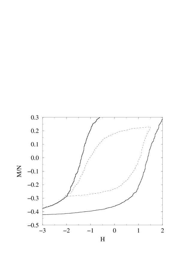
FIG. 7.: Example of a hysteresis loop of model B showing the failure of the return point memory property after partial cycling. Data corresponds to a simulation of a system with $\epsilon=-0.2$ and $L=10$.

FIG. 8.: Probability distribution $p(s)$ of avalanche sizes in the hysteresis loop of model A. Data corresponds to an average of 300 runs for a system with $L=30$ and different values of $\theta_{0}$ as indicated. Except for the bottom curve, the curves have been vertically shifted (three decades each) in order to clarify the picture. Continuous lines correspond to examples of the fits of equation (12).

FIG. 9.: Probability distribution of avalanche sizes in the hysteresis loop of model B. Data corresponds to an average of 100 runs for a system with $L=30$ and different values of $\epsilon$ as indicated. Except for the bottom curve, the curves have been vertically shifted (three decades) in order to clarify the picture.

FIG. 10.: Comparison of the histograms $N(s)$ (circles) and $N(\Delta M)$ (continuous line with black triangles indicating the centre of the logarithmic bin) corresponding to model A with a system size $L=20$ and with $\theta_{0}=1.39$. Data correspond to averages over $300$ different realizations.

FIG. 11.: Distribution of avalanches for model A with $L=20$ and $\theta_{0}=1.39$. Data corresponds to averages over $1000$ different configurations of disorder. The bottom histogram corresponds to the analysis of all avalanches. The top histogram (shifted 6 decades) corresponds to the spanning avalanches and the middle one (shifted 3 decades) to the non-spanning avalanches. The inset shows the histogram of spanning avalanches on a linear scale. Data in the inset has been smoothed in order to clarify the picture.

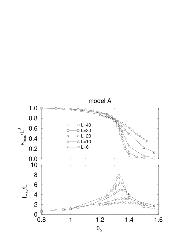
FIG. 12.: Average size (a) and duration (b) of the largest avalanche in the full hysteresis loop as a function of the amount of disorder $\theta_{0}$ for model A. Data correspond to different system sizes as indicated by the legend and to averages over many different configurations of disorder.

FIG. 13.: Average size (a) and duration (b) of the largest avalanche in the full hysteresis loop as a function of the amount of disorder $\epsilon$ for model B.

FIG. 14.: Fitted parameters $\lambda$ and $\tau^{\prime}$ to the avalanche size distributions as defined in equation 12 for model A. Data correspond to different system sizes as indicated by the legend and to averages over many different configurations of disorder.

FIG. 15.: Fitted parameters $\lambda$ and $\tau^{\prime}$ to the avalanche size distributions as defined in equation 12 for model B. Data correspond to different system sizes as indicated by the legend and to averages over many different configurations of disorder.

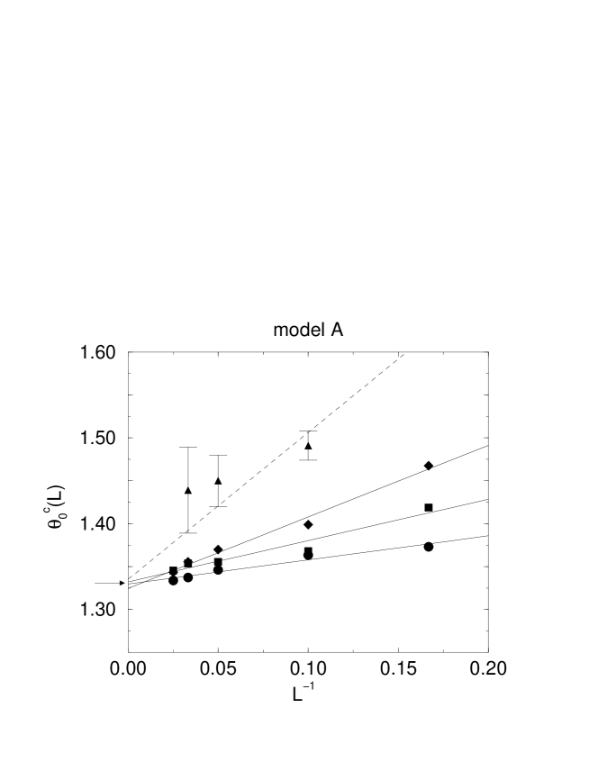
FIG. 16.: Dependence of different estimations of $\theta_{0}^{c}(L)$ on $L^{-1}$ for model A. Circles correspond to the estimations from the position of the maximum in $t_{max}(\theta_{0})$, diamonds to the position of the inflection point in $s_{max}(\theta_{0})$, squares to the position of the minimum in the numerical derivative $ds_{max}(\theta_{0})/d\theta_{0}$, and triangles to the disorder values for which the parameter $\lambda$ vanishes. Continuous lines correspond to linear fits used for the extrapolation to $L\rightarrow\infty$. The dashed line is a guide to the eye. The arrow indicates the value $\theta_{c}=1.33$.

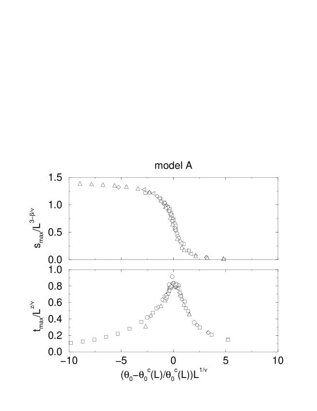
FIG. 17.: Scaling of the largest avalanche size $s_{max}(\theta_{0},L)$ and duration of the longest avalanche $t_{max}(\theta_{0},L)$ for model A. The values $\nu=1$, $\beta=0.1$ and $z=1.6$ have been used.

FIG. 18.: Scaling of the largest avalanche size $s_{max}(\epsilon,L)$ and duration of the longest avalanche $t_{max}(\epsilon,L)$ for model B. The values $\nu=1$, $\beta=0.1$ and $z=1.6$ have been used.

FIG. 19.: Avalanche size distribution corresponding to different values of the applied external field $H$ for model A with size $L=20$ and $\theta_{0}=1.39$. Histograms have been performed by counting the avalanches within a window of $\Delta H=0.5$ centred on different values of the field. From bottom to top such fields vary from $0.0$ to $-2.25$ with steps of $0.25$. Moreover, averages over $1000$ realizations of disorder have been performed. Histograms have been shifted two decades each in order to clarify the picture.

FIG. 20.: Parameters $\lambda$ and $\tau$ as a function of the external field $H$ fitted from the histograms in figure 19, corresponding to a system with size $L=20$ and $\theta_{0}=1.39$

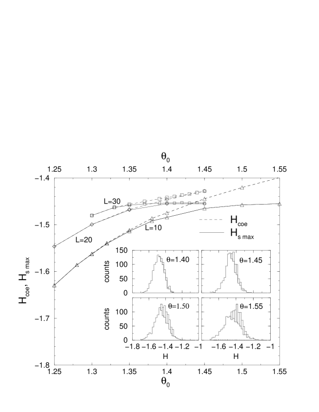
FIG. 21.: Comparison of the dependence of the coercive field $\langle H_{coe}\rangle$ and the field for which the largest avalanche occurs $\langle H_{s_{max}}\rangle$ as a function of the amount of disorder $\theta_{0}$ for model A with $L=10$, $20$ and $30$. Inset show the actual distribution of the two quantities ($\langle H_{coe}\rangle$ with an empty histogram and $\langle H_{s_{max}}\rangle$ with a lined histogram) for $L=10$ at four values of the amount of disorder as indicated.