Irreversible Bimolecular Reactions of Langevin Particles

Abstract

The reaction $A+B\,\longrightarrow\,B$ is studied when the reactants diffuse in phase space, i.e. their dynamics is described by the Langevin equation. The steady-state rate constants are calculated for both the target (static $A$ and mobile $B$’s) and trapping (mobile $A$ and static $B$’s) problems when the reaction is assumed to occur at the first contact. For Brownian dynamics (i.e., ordinary diffusion), the rate constant for both problems is a monotonically decreasing function of the friction coefficient $\gamma$. For Langevin dynamics, however, we find that the steady-state rate constant exhibits a turnover behavior as a function of $\gamma$ for the trapping problem but not for the target problem. This turnover is different from the familiar Kramers’ turnover of the rate constant for escape from a deep potential well because the reaction considered here is an activationless process.

I Introduction

Theories of bimolecular chemical reactions in solvents that occur at first contact of the reactants has been traditionally developed assuming that molecules move in diffusive manner [1]. This corresponds to the so-called high friction limit of the more general Langevin dynamics. In this paper we develop a theory for Langevin reactant dynamics and analyze the kinetics over the entire range of the friction coefficient, from low to high friction.

Specifically, we study the kinetics of the irreversible reaction $A+B\,\longrightarrow\,B$ in two limiting cases: static $A$ and mobile $B$’s (target problem) and mobile $A$ and static $B$’s (trapping problem); the difference between the two problems is illustrated in Fig. 1. Traditional theories based on the diffusion equation predict monotonic decrease of the reaction rate when the diffusion constant decreases, i.e. when the friction increases. It will be shown that in the case of the Langevin dynamics such a behavior of the reaction rate with the friction is observed only for the target problem. For the trapping problem the steady state rate constant has a turnover behavior as a function of the friction coefficient $\gamma$: it first increases with $\gamma$, reaches a maximum, turns over and then decreases approaching zero as $\gamma\rightarrow\infty$. This rate constant vanishes at $\gamma=0$ in one dimension while it remains finite in higher dimensions.

The turnover behavior of the reaction rate is well known in the Kramers’ theory of activated unimolecular reactions [2, 3]. This theory considers the escape of a Langevin particle from a deep potential well. To escape the particle has to overcome a high (compared to ${\rm k_{B}T}$) potential barrier. The escape rate vanishes as $\gamma\rightarrow 0$ and as $\gamma\rightarrow\infty$ and has a maximum in between. At low friction the rate is limited by energy exchange with the environment and vanishes at $\gamma=0$ since the particle cannot gain the energy necessary to overcome the barrier. As $\gamma$ becomes finite, the particle can exchange energy with the environment. This leads to the increase of the reaction rate. This is the so-called low friction or energy diffusion regime. In the opposite limiting case when $\gamma\rightarrow\infty$ (the high friction regime), particle’s motion is purely diffusive. As a consequence, the escape rate is proportional to the diffusion constant, $D={\rm k_{B}T}/\gamma$ so that the reaction rate vanishes when $D$ goes to zero.

In the trapping problem a particle does not need to overcome an energy barrier in order to react. In fact, even when the friction is zero every particle with finite initial velocity will eventually react. Of course, particles that move faster will be trapped more quickly and are the first to be removed from the system. When the friction increases from zero, these particles can be replaced by initially slower moving particles that gain energy from the heat bath. Thus the trapping rate at first increases as the friction increases. As the friction is further increased, the motion of the particle eventually becomes diffusive and in this limit the trapping rate is proportional to the diffusion coefficient $D$ which vanishes as the friction tends to infinity.

To analyze the kinetics when motion of the reactants is governed by the Langevin equation one has to solve the Klein-Kramers equation in the phase space with appropriate boundary conditions. This is an extremely complicated task. Even the simple problem of survival of a free particle moving on a line in the presence of a single trap has an extremely complicated solution in the phase space. This solution was found by Marshall and Watson [4] forty years later after the problem was posed by Wang and Uhlenbeck [5] in $1945$. A discussion of the source of this complexity and a list of key references can be found in Refs.[[4, 6]].

Since we cannot solve the problem in phase space exactly we will find approximate solutions in the limiting cases of low and high friction. These solutions are then used to construct an interpolation formula that covers the entire range of the friction coefficient. The outline of the paper is as follows. In section II we analyze the survival of a Langevin particle moving on a line between two static traps. Some of results derived in this section has been reported earlier [7] without derivation. An approximate solution found in Section II is used in Section III to calculate the steady-state rate constant for the trapping problem in one dimension over the entire range of the friction coefficient. Since this approach is not generalizable to higher dimensions, in Section IV we develop another approximate method that can be applied in a space of arbitrary dimension and use it in Section V to find the rate constants for the target and trapping problems as a function of the friction coefficient in one and three dimensions. Section VI contains a brief summary.

II Survival on an Interval Terminated by Trapping Points

In this section we analyze the survival of a Langevin particle moving on a line between two traps. We calculate the effective rate constant characterizing the kinetics of trapping. By averaging this rate with respect to the length of the interval, we will obtain the steady-state rate constant for the trapping problem in one dimension over the entire range of the friction.

Let $x$ and $\dot{x}=v$ denote the position and velocity of a free particle of unit mass whose dynamics is governed by the Langevin equation,

$$\ddot{x}+\gamma\,\dot{x}=R(t)\>,$$ (2.1)

where $\gamma$ is the friction coefficient and $R(t)$ is a Gaussian random force of zero mean with correlation function given by the fluctuation-dissipation relation, $\langle R(t)R(t^{\prime})\rangle=2\,\gamma\,\delta(t-t^{\prime})$. Here and below the thermal energy is set ${\rm k_{B}T}=1$.

Equivalently, the joint probability density, $P(x,v,t)$, of finding the particle at the phase space point $(x,v)$ at time $t$ is described by the Klein-Kramers equation:

$$\frac{\partial P(x,v,t)}{\partial t}=\left[-v\,\frac{\partial}{\partial x}\,+\,\gamma\,\frac{\partial}{\partial v}\,{\rm e}^{-v^{2}/2}\,\frac{\partial}{\partial v}\,{\rm e}^{v^{2}/2}\right]\,P(x,v,t)\>.$$ (2.2)

To study the escape of the Brownian particle from the interval $[0,1]$, we require that $P(x,v,t)$ satisfies the absorbing boundary conditions:

$$\left\{\begin{array}[]{lcc}P(x,v>0,t)=0&\mbox{at}&x=0\>,\\ P(x,v<0,t)=0&\mbox{at}&x=1\>.\end{array}\right.$$ (2.5)

Assuming that the system has initially a uniform spatial distribution and the Maxwell velocity distribution, the survival probability that describes the fate of the particle in the interval is given by,

$$S(t)=\int_{0}^{1}\!dx\int_{-\infty}^{+\infty}\!dv\,P(x,v,t)\>,$$ (2.6)

where $P(x,v,t)$ is the solution of Eq.(2.2) with initial condition $P(x,v,t=0)=p_{\rm eq}(x)\,f_{\rm eq}(v)$, with $p_{\rm eq}(x)=1$ and

$$f_{\rm eq}(v)=\frac{{\rm e}^{-v^{2}/2}}{\sqrt{2\pi}}\>.$$ (2.7)

To characterize the kinetics of the escape from the interval we will use the effective rate constant, $k$, defined as the reciprocal of the mean lifetime of the particle on the interval,

$$\frac{1}{k}=\int_{0}^{\infty}\!S(t)\,dt\>.$$ (2.8)

When $\gamma=0$, the particle moves with a constant velocity. The survival probability of a particle starting at $x$ with a velocity $v$ is,

$$S(t|x,v)={\rm H}(-v)\,{\rm H}\left[x+vt\right]+{\rm H}(v)\,{\rm H}\left[x-1-vt\right]\>,$$ (2.9)

where ${\rm H}(z)$ is the Heaviside step function defined as ${\rm H}(z)=0$ for $z<0$ and ${\rm H}(z)=1$ for $z>0$. Averaging $S(t|x,v)$ over the uniform distribution in $x$ and the equilibrium distribution in $v$ gives:

$$S(t)=\int_{0}^{1}\!dx\int_{-\infty}^{+\infty}\!S(t|x,v)\,f_{\rm eq}(v)\,dv={\rm erf}\left[\frac{1}{\sqrt{2}\>t}\right]\,-\,\sqrt{\frac{2}{\pi}}\>t\,\left[1-{\rm e}^{-1/(2t^{2})}\right]\>.$$ (2.10)

This expression shows that in the ballistic limit, $S(t)$ has a power law tail

$$S(t)\simeq\frac{1}{\sqrt{2\pi}\>t}\>\>\>;\>\>\>t\rightarrow\infty\>.$$ (2.11)

From this and the definition in Eq.(2.8) it follows that $k=0$ when $\gamma=0$.

On the other hand, when $\gamma=\infty$, the particle does not move and $S(t)=1$. As a consequence, $k=0$ in this limiting case also. Since $k$ vanishes in the $\gamma\rightarrow 0$ and $\gamma\rightarrow\infty$ limits, this rate constant shows a turnover behavior as a function of $\gamma$.

Since the solution of Eq.(2.2) with boundary conditions (2.5) is unknown, we adopt the following strategy for determining $k$ for arbitrary values of $\gamma$. We first derive approximate expressions for $k$ in high and low friction regimes, and then use the Visscher-Mel’nikov-Meshkov [3, 8] (VMM) interpolation formula to obtain an expression for the rate constant that covers the entire range of $\gamma$.

A High Friction Regime

In this section, we analyze the the high friction limit. First, we reduce the Klein-Kramers equation (2.2) with absorbing boundary conditions (2.5) to the ordinary diffusion equation with radiation boundary conditions. Next, we calculate the effective rate constant by solving this equation.

To proceed, we define the reduced probability density,

$$p(x,t)=\int_{-\infty}^{+\infty}\!P(x,v,t)\,dv\>,$$ (2.12)

and the flux,

$$j(x,t)=\int_{-\infty}^{+\infty}\!v\,P(x,v,t)\,dv\>.$$ (2.13)

Integration of Eq.(2.2) over the velocity leads to the continuity equation:

$$\frac{\partial p(x,t)}{\partial t}=-\,\frac{\partial j(x,t)}{\partial x}\>,$$ (2.14)

in which we have used $P(x,\pm\infty,t)=0$. Multiplying Eq.(2.2) by $v$ and integrating over the velocity from $-\infty$ to $+\infty$, we have:

$$\frac{\partial j(x,t)}{\partial t}=-\gamma\,j(x,t)\,-\,\int_{-\infty}^{+\infty}\!v^{2}\,\frac{\partial P(x,v,t)}{\partial x}\,dv\>.$$ (2.15)

This equation can easily be solved to give:

$$j(x,t)={\rm e}^{-\gamma t}\,j(x,0)\,-\,\int_{0}^{t}\!dt^{\prime}\,{\rm e}^{-\gamma(t-t^{\prime})}\,\int_{-\infty}^{+\infty}\!v^{2}\,\frac{\partial P(x,v,t^{\prime})}{\partial x}\,dv\>.$$ (2.16)

Note that since the initial distribution of the velocity is Maxwellian, we have $j(x,0)=0$. In the $\gamma\gg 1$ limit, $P(x,v,t^{\prime})$ does not vary on times of order of $1/\gamma$. Therefore, the integration over $t^{\prime}$ can be carried out easily to give:

$$j(x,t)=-\frac{1}{\gamma}\,\int_{-\infty}^{+\infty}\!v^{2}\,\frac{\partial P(x,v,t)}{\partial x}\,dv\>.$$ (2.17)

Plugging this into Eq.(2.14) leads to:

$$\frac{\partial p(x,t)}{\partial t}=\frac{1}{\gamma}\,\int_{-\infty}^{\infty}\!v^{2}\,\frac{\partial^{2}P(x,v,t)}{\partial x^{2}}\,dv\>.$$ (2.18)

In the $\gamma\gg 1$ limit, $P(x,v,t)$ can be written as an expansion in powers of $1/\gamma$. The zero order term of this expansion is,

$$P(x,v,t)=f_{\rm eq}(v)\,p(x,t)\>.$$ (2.19)

Using this in Eq.(2.18) one obtains the ordinary one-dimensional diffusion equation,

$$\frac{\partial p(x,t)}{\partial t}=D\,\frac{\partial^{2}p(x,t)}{\partial x^{2}}\>\>\>;\>\>\>D=\frac{1}{\gamma}\>.$$ (2.20)

To derive boundary conditions supplementing this equation we use the two expressions for the flux given in Eqs.(2.13) and (2.17) to write:

$$j(x,t) = \int_{-\infty}^{0}\!v\,P(x,v,t)\,dv+\int_{0}^{\infty}\!v\,P(x,v,t)\,dv$$ (2.21)

$$= -\frac{1}{\gamma}\,\int_{-\infty}^{0}\!v^{2}\,\frac{\partial P(x,v,t)}{\partial x}\,dv\,-\,\frac{1}{\gamma}\,\int_{0}^{\infty}\!v^{2}\,\frac{\partial P(x,v,t)}{\partial x}\,dv\>,$$ (2.22)

where the integral over the velocity has been broken into two parts. At the boundaries, according to Eq.(2.5), $P(0,v>0,t)=P(1,v<0,t)=0$. This suggests that $\left.\partial P(x,v>0,t)/\partial x\right|_{x=0}$ is much larger than $\left.\partial P(x,v<0,t)/\partial x\right|_{x=0}$, and $\left.\partial P(x,v<0,t)/\partial x\right|_{x=1}$ is much larger than $\left.\partial P(x,v>0,t)/\partial x\right|_{x=1}$, when $|v|$ is not too small. Since contribution of small velocities are weakened by the multiplying factor $v^{2}$, we neglect these small terms. Retaining only major contributions leads to:

$$j(0,t)=\left.\left(-\frac{1}{\gamma}\,\int_{0}^{\infty}\!v^{2}\,\frac{\partial P(x,v,t)}{\partial x}\,dv\right)\right|_{x=0} = \int_{-\infty}^{0}\!v\,P(0,v,t)\,dv\>,$$ (2.23a)

$$j(1,t)=\left.\left(-\frac{1}{\gamma}\,\int_{-\infty}^{0}\!v^{2}\,\frac{\partial P(x,v,t)}{\partial x}\,dv\right)\right|_{x=1} = \int_{0}^{\infty}\!v\,P(1,v,t)\,dv\>.$$ (2.23b)

Substituting the approximation for $P(x,v,t)$ given in Eq.(2.19) into these relations, we obtain the radiation boundary conditions:

$$\left.D\,\frac{\partial p(x,t)}{\partial x}\right|_{x=0}=\kappa\,\,p(0,t)\>,$$ (2.24a)

$$\left.-D\,\frac{\partial p(x,t)}{\partial x}\right|_{x=1}=\kappa\,p(1,t)\>,$$ (2.24b)

where $\kappa$ is defined as,

$$\kappa=\langle|v|\rangle=\int_{-\infty}^{\infty}\!|v|\,f_{\rm eq}(v)\,dv=\frac{1}{\sqrt{2\pi}}\int_{-\infty}^{\infty}\!|v|\,{\rm e}^{-v^{2}/2}\,dv=\left(\frac{2}{\pi}\right)^{1/2}=0.7979\>.$$ (2.25)

Using $\kappa$ given by Eq.(2.25), one can find the corresponding Milne’s length, $l=D/\kappa=1.253/\gamma$, which has to be compared with the exact value, $l=-\zeta(1/2)\,D=1.46/\gamma$ (where $\zeta(z)$ is the zeta function [9]), obtained from a very sophisticated derivation [4]. The two Milne’s lengths are in a reasonably good agreement, considering the simplicity of our derivation.

The survival probability $S_{\rm high}(t)$ (where the subscript ”high” designates the high friction regime) is :

$$S_{\rm high}(t)=\int_{0}^{1}\!p(x,t)\,dx\>,$$ (2.26)

where $p(x,t)$ is the solution of Eq.(2.20) with the initial condition $p(x,t=0)=1$ and boundary conditions (2.24a) and (2.24b). The mean lifetime, $k_{\rm high}^{-1}$, of a particle diffusing between partially absorbing boundaries and initially uniformly distributed on the interval is [10]:

$$\frac{1}{k_{\rm high}}=\frac{1}{k_{\rm eq}}\,+\,\frac{1}{k_{\rm d}}\>,$$ (2.27)

where $k_{\rm eq}$ is the rate constant in the reaction controlled limit (i.e., $\gamma\rightarrow 0$, $D\rightarrow\infty$ limit or $\kappa\rightarrow 0$) given by:

$$k_{\rm eq}=\kappa\,p_{\rm eq}(0)+\kappa\,p_{\rm eq}(1)=2\kappa\>.$$ (2.28)

The second term $k_{\rm d}$ in Eq.(2.27) is the rate constant in the diffusion controlled limit (i.e., $\gamma\rightarrow\infty$, $D\rightarrow 0$ limit or $\kappa\rightarrow\infty$) which is the inverse of the mean first passage time of the particle to the boundaries at $x=0$ and $x=1$, averaged over the uniform distribution of initial positions:

$$k_{\rm d}^{-1}=\frac{1}{12D}=\frac{\gamma}{12}\>.$$ (2.29)

Plugging this and the expression in Eq.(2.28) into Eq.(2.27), we find that the effective rate constant is:

$$\frac{1}{k_{\rm high}}=\frac{1}{2\kappa}\,+\,\frac{1}{12D}=\frac{1}{2\kappa}\,+\,\frac{\gamma}{12}\>.$$ (2.30)

B Low Friction Regime

In this section we analyze the low friction regime where $\gamma$ is small and, hence, the particle velocity is a slowly varying variable. First, we reduce the Klein-Kramers equation (2.2) with the absorbing boundary conditions (2.5) to a diffusion equation along the velocity coordinate in the presence of a sink term describing the escape of the particle from the interval. Next, we calculate the effective rate constant by solving this equation.

When $\gamma=0$, the survival probability of a particle starting at $x$ with initial velocity $v$ is given by Eq.(2.9), and the lifetime of such a particle is given by:

$$\int_{0}^{\infty}\!S(t|x,v)\,dt=\frac{x}{|v|}\,{\rm H}(-v)+\frac{(1-x)}{v}\,{\rm H}(v)\>.$$ (2.31)

Averaging this time with respect to uniform distribution of $x$ gives the mean lifetime, $1/K(v)$,

$$\frac{1}{K(v)}=\int_{0}^{1}\!dx\int_{0}^{\infty}\!S(t|x,v)\,dt=\frac{1}{2|v|}\>.$$ (2.32)

$K(v)$ can be regarded as the effective rate constant for the escape of a particle with initial velocity $v$.

Let $f(v,t)$ be the probability density of the velocity. For finite $\gamma$ and in the absence of any reaction leading to the depletion of the probability density, $f(v,t)$ satisfies the differential equation,

$$\frac{\partial f(v,t)}{\partial t}=\gamma\,\frac{\partial}{\partial v}\,{\rm e}^{-v^{2}/2}\,\frac{\partial}{\partial v}\,{\rm e}^{v^{2}/2}\,f(v,t)\>.$$ (2.33)

This equation describes the relaxation of $f(v,t)$ to the Maxwell distribution, $f_{\rm eq}(v)$, in Eq.(2.7). Because of the escape of particles from the interval, the probability density of the velocity decreases with time. The simplest way of taking this decrease into account is to incorporate a sink term into Eq.(2.33) as,

$$\frac{\partial f(v,t)}{\partial t}=\gamma\,\frac{\partial}{\partial v}\,{\rm e}^{-v^{2}/2}\,\frac{\partial}{\partial v}\,{\rm e}^{v^{2}/2}\,f(v,t)\,-\,K(v)\,f(v,t)\>,$$ (2.34)

where $K(v)$ is chosen so that in the limit $\gamma\rightarrow 0$, the mean lifetime of the particle given in Eq.(2.32) is recovered, i.e., $K(v)=2|v|$.

The survival probability $S_{\rm low}(t)$ is given by

$$S_{\rm low}(t)=\int_{-\infty}^{\infty}\!f(v,t)\,dv\>,$$ (2.35)

where $f(v,t)$ is the solution of Eq.(2.34) with the initial condition $f(v,t=0)=f_{\rm eq}(v)$. When $\gamma=0$, the survival probability obtained by solving Eq.(2.34) is,

$$S_{\rm low}(t)=\int_{-\infty}^{\infty}\!f_{\rm eq}(v)\,{\rm e}^{-K(v)\,t}\,dv=\int_{-\infty}^{\infty}\!\frac{{\rm e}^{-v^{2}/2}}{\sqrt{2\pi}}\,{\rm e}^{-2\,|v|\,t}\,dv={\rm e}^{2t^{2}}\,{\rm erfc}\left(\sqrt{2}\>t\right)\>.$$ (2.36)

This function turns out to have exactly the same long time behavior like the exact survival probability given in Eq.(2.11). As shown in Fig. 3, the two survival probabilities essentially coincide except for short times.

Integration of Eq.(2.34) with respect to $v$ gives the time derivative of $S_{\rm low}(t)$ at $t=0$ as:

$$-\left.\frac{dS_{\rm low}}{dt}\right|_{t=0}=\int_{-\infty}^{\infty}\!K(v)\,f_{\rm eq}(v)\,dv=2\langle|v|\rangle=2\kappa=k_{\rm eq}\>.$$ (2.37)

One can check that $dS_{\rm low}/dt=dS_{\rm high}/dt$ at $t=0$. Another interesting limit of Eq.(2.34) is when $\gamma\rightarrow\infty$. In this case, the velocity distribution instantaneously relaxes to $f_{\rm eq}(v)$ so that the probability density can be written as, $f(v,t)=f_{\rm eq}(v)\,S_{\rm low}(t)$, and the survival probability decays exponentially, $S_{\rm low}(t)={\rm e}^{-k_{\rm eq}t}$. From this it follows that the effective rate constant is equal to $k_{\rm eq}$ in the $\gamma\rightarrow\infty$ limit.

1 Effective Rate Constant

Let $\tau(v)$ be the lifetime of the particle initially with velocity $v$ in the presence of the sink term, $K(v)$. The effective rate constant in the low friction regime can be expressed in terms of $\tau(v)$ as

$$k_{\rm low}^{-1}=\int_{-\infty}^{+\infty}\!\tau(v)\,f_{\rm eq}(v)\,dv\>.$$ (2.38)

The lifetime $\tau(v)$ satisfies the adjoint equation,

$$\gamma\,{\rm e}^{v^{2}/2}\,\frac{d}{dv}\,{\rm e}^{-v^{2}/2}\,\frac{d\tau(v)}{dv}\,-\,2\,|v|\,\tau(v)=-1\>.$$ (2.39)

The boundary conditions that complement this equation are: $\tau(v)$ vanishes as $|v|\rightarrow\infty$ and $\left.d\tau(v)/dv\right|_{v=0}=0$, since $\tau(v)$ is a symmetric function of $v$, i.e. $\tau(-v)=\tau(v)$.

When $\gamma$ is small, Eq.(2.39) can be solved approximatively by matching the solutions found for small and large $v$. For large velocities, $|v|>v^{\ast}$, where $v^{\ast}$ is a constant to be determined, the second term in Eq.(2.39) is more important than the first one (since $\gamma$ is small) and so $\tau(v)\simeq 1/2|v|$. At small $v$, the second term, proportional to $v$, can be neglected and the exponentials can be replaced by unity. Thus, Eq.(2.39) takes the form

$$\gamma\,\frac{d^{2}\tau(v)}{dv^{2}}=-1\>\>\>;\>\>\>|v|\leq v^{\ast}\>.$$ (2.40)

The solution satisfying the condition $\left.d\tau(v)/dv\right|_{v=0}=0$ is

$$\tau(v)=\tau(0)-\frac{v^{2}}{2\gamma}\>.$$ (2.41)

The time $\tau(0)$ and the velocity $v^{\ast}$ are determined from the condition of continuity of $\tau(v)$ and $d\tau(v)/dv$ at $v=v^{\ast}$. This leads to

$$\tau(v)=\left\{\begin{array}[]{lcc}1/2v^{\ast}+(v^{\ast\,2}-v^{2})/2\gamma&;&0\leq|v|\leq v^{\ast}\>,\\ 1/2|v|&;&|v|\geq v^{\ast}\>,\end{array}\right.$$ (2.44)

where $v^{\ast}=(\gamma/2)^{1/3}$.

Averaging $\tau(v)$ with respect to $f_{\rm eq}(v)$, one finds that the leading term of $k_{\rm low}(\gamma)$ as $\gamma\rightarrow 0$ is:

$$k_{\rm low}\approx 3\sqrt{2\pi}\,\left[\ln\left(\frac{1}{\gamma}\right)\right]^{-1}=\frac{3\pi}{2}\,\left[\ln\left(\frac{1}{\gamma}\right)\right]^{-1}\,k_{\rm eq}\>.$$ (2.45)

This result is exact and can be derived directly from Eq.(2.2) with appropriate boundary conditions. Since $k_{\rm low}=k_{\rm eq}$ as $\gamma\rightarrow\infty$, the following heuristic formula can be used to interpolate $k_{\rm low}$ over the entire range of $\gamma$:

$$k_{\rm low}=k_{\rm eq}\,\left\{1+\frac{2}{3\pi}\,\ln\left[1+\frac{A}{\gamma}\right]\right\}^{-1}\>,$$ (2.46)

in which $A$ is the only unknown constant. It is found that Eq.(2.46) accurately fits exact results (obtained by solving Eq.(2.39) numerically) for $A=1.45$.

C Turnover

So far we have derived expressions for $k_{\rm low}$ and $k_{\rm high}$ as functions of $\gamma$. Now, we use the VMM [3, 8] interpolation formula to obtain an analytic expression for $k$ that covers the entire range of $\gamma$. This leads to

$$\frac{k(\gamma)}{k_{\rm eq}}=\frac{k_{\rm low}(\gamma)\,k_{\rm high}(\gamma)}{k_{\rm eq}^{2}}=\left\{\left[1+\frac{2}{3\pi}\,\ln\left(1+\frac{A}{\gamma}\right)\right]\,\left[1+\frac{\gamma}{\sqrt{18\pi}}\right]\right\}^{-1}\>.$$ (2.47)

In order to test the theory, we have performed Langevin dynamics simulations to compute the exact survival probability, $S(t)$, and the effective rate constant, $k$, as described in Appendix A. The results are reported in Fig. 2 where the closed circles represent simulation data, solid and dashed lines give the dependences predicted by Eq.(2.47) with $A=1.45$ and $A=6$, respectively, while dot-dashed and long-dashed lines display $k_{\rm high}$ (Eq.(2.30)) and $k_{\rm low}$ (Eq.(2.46)) with $A=1.45$, respectively. The dotted line designates the purely diffusive part of $k_{\rm high}$ (see Eq.(2.30)).

The rate constant shows a turnover behavior as a function of $\gamma$. In the low friction regime, it goes to zero like $k\sim 1/\ln(\gamma^{-1})$, in contrast to the Kramers’ rate constant which is proportional to $\gamma$. The theory, i.e. Eq.(2.47) with $A=1.45$, describes simulation results reasonably well. However, Eq.(2.47) with $A=6$ is in excellent agreement with the simulation data as shown by the dashed line through the data in Fig. 2. Equation (2.47) with $A=6$ can be regarded as exact for practical purposes. The rate constant $k$ increases as $\gamma$ gets larger, attains its maximum value (smaller than $k_{\rm eq}$) close to $\gamma\simeq 1$, turns over and then decreases like $k\sim\gamma^{-1}$ as $\gamma\rightarrow\infty$. In this friction regime, the theory is in excellent agreement with simulation results. Comparison between the dot-dashed and dotted lines (i.e., diffusion with perfectly absorbing boundary conditions) shows how results are improved by using radiation boundary conditions.

In Fig. 3, $S(t)$ is plotted versus $t$ for various values of $\gamma$. When $\gamma=0$, the survival probability is strongly non-exponential and goes as $t^{-1}$ at long times (see Eq.(2.11)). For comparison we have also plotted $S_{\rm low}(t)$ given in Eq.(2.36). As one can see, $S_{\rm low}(t)$ is slightly below $S(t)$ at short times (since the slopes at $t=0$ are $2\kappa$ and $\kappa$, respectively), but they become indistinguishable from each other at longer times.

For $\gamma=\infty$, $S(t)=1$ since the particle cannot reach the absorbing boundaries. When $\gamma=1$, the decay of $S(t)$ is close to exponential but with a slope smaller than $k_{\rm eq}=2\kappa$ represented by ${\rm e}^{-2\kappa t}$ (dot-dashed line). As $\gamma$ becomes smaller than unity, $S(t)$ becomes more and more non-exponential and decays very slowly. When $\gamma$ becomes greater than unity, $S(t)$ is almost an exponential with the slope $k_{\rm high}$ given in Eq.(2.30).

To summarize, the main result of this section is the expression given in Eq.(2.47) for the effective rate constant for a particle moving between two absorbing boundaries. It describes the turnover behavior of the rate constant as a function of $\gamma$. We will use this result in the next section to obtain the turnover of the steady-state rate constant in the trapping problem.

III Steady-State Rate Constant for the Trapping Problem in One Dimension

Consider an ensemble of traps (absorbing points) uniformly distributed on an infinite line. If $c$ is the concentration of traps (i.e., the number of traps per unit of length) and $L$ denotes the distance between neighboring traps, the distribution of $L$ is given by, $c\,{\rm e}^{-cL}$. A Langevin particle is injected at any point of the line with equal probability. The probability density that a particle is injected on the interval of length $L$ is $c^{2}L\,{\rm e}^{-cL}$. Let $s(t|L)$ be the survival probability of the particle moving within the interval $L$ averaged over uniform distribution of the initial position within the interval and over the equilibrium distribution of the initial velocity. Averaging $s(t|L)$ with respect to $L$, gives the survival probability of the particle in the presence of static traps at concentration $c$:

$${\cal S}(t)=c^{2}\int_{0}^{\infty}\!L\,{\rm e}^{-cL}\,s(t|L)\,dL\>.$$ (3.1)

Before analyzing the turnover of the steady-state rate constant as a function of $\gamma$, we briefly consider the asymptotic long time behavior of ${\cal S}(t)$, which is determined by particles located in large intervals free from traps. Such a particle changes its velocity many times before being trapped. As a consequence, the particle motion is essentially diffusive and its averaged survival probability approaches zero as ${\rm e}^{-t^{1/3}}$ at very long times [11].

The steady-state rate constant, $k_{\rm ss}$, is expressed in terms of the survival probability as,

$$k_{\rm ss}^{-1}=c\int_{0}^{\infty}\!{\cal S}(t)\,dt=c^{3}\int_{0}^{\infty}\!dt\int_{0}^{\infty}\!L\,{\rm e}^{-cL}\,s(t|L)\,dL\>.$$ (3.2)

Changing variables so as to express $s(t|L)$ in terms of the survival probability on a unit interval and carrying out the integration over the time, we have:

$$k_{\rm ss}(\varepsilon)=\left[\int_{0}^{\infty}\!\frac{z^{2}\,{\rm e}^{-z}}{k(\varepsilon z)}\,dz\right]^{-1}\>\>\>;\>\>\>\varepsilon=\frac{\gamma}{c}\>,$$ (3.3)

where $k(\varepsilon z)$ is the effective rate constant given in Eq.(2.47). Using this expression we find:

$$\frac{k_{\rm ss}(\varepsilon)}{\kappa}=\left[1+\frac{\varepsilon}{\sqrt{2\pi}}+\frac{1}{3\pi}\,h_{1}\left(\frac{A}{\varepsilon}\right)+\frac{\varepsilon}{9\pi\sqrt{2\pi}}\,h_{2}\left(\frac{A}{\varepsilon}\right)\right]^{-1}\>,$$ (3.4)

in which the functions $h_{1}(y)$ and $h_{2}(y)$ are defined as,

$$h_{1}(y) = 2\gamma_{\rm E}+2\ln(y)-y+\left[y^{2}-2y+2\right]\,{\rm e}^{y}\,{\rm E}_{1}(y)\>,$$ (3.5a)

$$h_{2}(y) = 6\gamma_{\rm E}+6\ln(y)-4y+y^{2}-\left[y^{3}-3y^{2}+6y-6\right]\,{\rm e}^{y}\,{\rm E}_{1}(y)\>,$$ (3.5b)

where $\gamma_{\rm E}=0.577216$ is the Euler’s constant and, ${\rm E}_{1}(y)=\int_{y}^{\infty}\!z^{-1}\,{\rm e}^{-z}\,dz$, is the exponential integral function [9].

Equation (3.4) predicts a turnover behavior of the steady-state rate constant as a function of $\varepsilon$. When $\varepsilon\rightarrow 0$, $k_{\rm ss}$ approaches zero as

$$\frac{k_{\rm ss}(\varepsilon)}{\kappa}\simeq\frac{3\pi}{2}\,\left[\ln\left(\frac{B}{\varepsilon}\right)\right]^{-1}\>\>\>;\>\>\>B=A\,\exp\left\{\frac{3\pi-3+2\gamma_{\rm E}}{2}\right\}\>.$$ (3.6)

In the opposite limit when $\varepsilon\rightarrow\infty$, the steady-state rate constant tends to zero like,

$$\frac{k_{\rm ss}(\varepsilon)}{\kappa}\simeq\frac{\sqrt{2\pi}}{\varepsilon}\>.$$ (3.7)

In Fig. 4 the $\varepsilon$-dependence of $k_{\rm ss}(\varepsilon)$ given in Eq.(3.4) is shown for $A=6$ (solid curve) and $A=1.45$ (dashed curve). The former may be considered as exact since it is obtained with $A=6$, which provides an almost perfect fit to simulation data for the unit interval (see Fig. 2). The dashed curve shows the dependence obtained on the basis of the theory developed in Section II B. Although both curves have the same qualitative behavior there is clearly a room for improvement. In what follows we develop another approach which allows one to calculate $k_{\rm ss}(\varepsilon)$ in a space of arbitrary dimension. We will use the dependence shown by the solid curve in Fig. 4 in order to test the approach in one dimension. It will be shown that the new theory predicts the dependence of $k_{\rm ss}(\varepsilon)$ which is in better agreement with the exact result (solid curve in Fig. 4) than does the theory developed in Section II B (dashed curve in Fig. 4).

IV New Approach

We now introduce a new and simpler approach to calculate the steady-state rate constant for the trapping problem which has the great advantage of being generalizable to any dimensions. Moreover, this approximate approach is expected to improve as the dimension of the space increases. As we will see below, even in one dimension, the new approach is already in better agreement with the simulations than does the previous one (compare Figs. 4 and 5).

The basic idea of this new approach is to apply the VMM interpolation formula directly to the steady-state rate constants found in the low and high friction regimes. In the low friction regime the rate constant will be obtained by using a many-particle generalization of the approach presented in Section II B. In the high friction regime we will assume that the steady-state rate constant for the trapping problem is equal to the rate constant for the target problem. This approximation is quite good in one dimension and is virtually exact in three dimensions.

A Target Problem

The survival probability of the target particle (i.e., the $A$ in the reaction $A+B\,\longrightarrow\,B$ with $D_{A}=0$), is given by

$${\cal S}_{\rm targ}(t)=\exp\left\{-c\int_{0}^{t}k_{\rm targ}(t^{\prime})\,dt^{\prime}\right\}\>,$$ (4.1)

where $c$ is the concentration of mobile traps (i.e., the $B$’s) and $k_{\rm targ}(t)$ is the time-dependent rate coefficient. The steady-state rate constant is [12]

$$k_{\rm targ}^{-1}=c\int_{0}^{\infty}\!{\cal S}_{\rm targ}(t)\,dt\>.$$ (4.2)

The exact time-dependent rate coefficient $k_{\rm targ}(t)$ is obtained by solving the Klein-Kramers equation with appropriate boundary conditions. This is an extremely complicated problem [13] and here we will approximate $k_{\rm targ}(t)$ by the Collins-Kimball rate constant, $k_{\rm CK}(t)$, which is obtained by solving the diffusion equation with the radiation boundary condition at contact, in which the intrinsic rate constant is chosen so that $k_{\rm CK}(0)$ is exact.

First, we note that $k_{\rm targ}(t=0)$ can be found exactly for any friction. The product $ck_{\rm targ}(0)$ is just the collision frequency, therefore

$$k_{\rm targ}(0)=\kappa=\left\{\begin{array}[]{ccc}\langle|v|\rangle=\sqrt{2/\pi}&;&d=1\>,\\ \pi R^{2}\,\langle|v|\rangle=\sqrt{8\pi}\>R^{2}&;&d=3\>,\end{array}\right.$$ (4.5)

where $R$ is the contact radius. In addition, when the friction vanishes, $\gamma=0$, $k_{\rm targ}(t)=k_{\rm targ}(0)$ and thus the rate constant is given by Eq.(4.5) for all times. As the friction tends to infinity, the rate constant is given by the Smoluchowski theory. Now, we consider the Collins-Kimball rate coefficient, $k_{\rm CK}(t)$, obtained for the diffusion constant $D=1/\gamma$ and the intrinsic rate constant $\kappa$ appearing in the boundary conditions equal to $k_{\rm targ}(0)$ given in Eq.(4.5). This Collins-Kimball rate coefficient has the following properties: i) $k_{\rm CK}(0)=k_{\rm targ}(0)$ at any friction, ii) when the friction vanishes, we have $k_{\rm CK}(t)=k_{\rm targ}(0)$ for all times, and iii) at high friction $k_{\rm CK}(t)$ coincides with the Smoluchowski rate constant except for very short times where it is equal to $k_{\rm targ}(0)$. In the view of these properties we approximate $k_{\rm targ}(t)$ by $k_{\rm CK}(t)$. As a consequence, we have ${\cal S}_{\rm targ}(t)={\cal S}_{\rm CK}(t)$ and

$$k_{\rm targ}^{-1}=c\int_{0}^{\infty}\!{\cal S}_{\rm CK}(t)\,dt\>.$$ (4.6)

B Trapping Problem in the Low Friction Regime

When the friction vanishes, the particle moves with a constant velocity. Its survival probability is equal to the probability that the region visited by the particle in time $t$ is free from traps. Since the traps are uniformly distributed in space, the probability that a region is free from traps is given by the Poisson distribution. The survival probability of a particle moving with a velocity $v$ is

$${\cal S}(t|v)=\left\{\begin{array}[]{lcc}\exp(-c|v|t)&;&d=1\>,\\ \exp(-c\pi R^{2}|v|t))&;&d=3\>.\end{array}\right.$$ (4.9)

Assuming equilibrium distribution of the initial velocity, the probability density of the velocity at time $t$ is

$$f(v,t)={\cal S}(t|v)\,f_{\rm eq}(v)\>.$$ (4.10)

Integrating this with respect to velocity, we find the survival probability in the ballistic regime

$${\cal S}_{\rm ball}(t)=\int\!f(v,t)\,dv=\int\!{\cal S}(t|v)\,f_{\rm eq}(v)\,dv\>.$$ (4.11)

This result is exact. In one dimension it leads to

$${\cal S}_{\rm ball}(t)=\left(\frac{2}{\pi}\right)^{1/2}\int_{0}^{\infty}\!\exp\left\{-cvt-\frac{v^{2}}{2}\right\}\,dv=\exp\left(\frac{c^{2}t^{2}}{2}\right)\,{\rm erfc}\left(\frac{ct}{\sqrt{2}}\right)\>.$$ (4.12)

This expression can also be obtained using $S(t)$ in Eq.(2.10) in the relation for ${\cal S}(t)$ given in Eq.(3.1). In three dimensions ${\cal S}_{\rm ball}(t)$ is

$${\cal S}_{\rm ball}(t) = \left(\frac{2}{\pi}\right)^{1/2}\int_{0}^{\infty}\!v^{2}\,\exp\left\{-c\pi R^{2}vt-\frac{v^{2}}{2}\right\}\,dv$$ (4.13)

$$= \left(1+\frac{\pi\tau^{2}}{8}\right)\,\exp\left(\frac{\pi\tau^{2}}{16}\right)\,{\rm erfc}\left(\frac{\sqrt{\pi}}{4}\,\tau\right)-\frac{\tau}{2}\>\>\>;\>\>\>\tau=\kappa ct=\sqrt{8\pi}\>cR^{2}t\>,$$ (4.14)

where we have used the relation in Eq.(4.5) for $\kappa$ in three dimensions, i.e. $\kappa=\sqrt{8\pi}\>R^{2}$.

Equations (4.9) and (4.10) show that particles with large velocities react more rapidly and therefore the higher the velocity the faster the probability density decays. When the friction is non-zero, due to the interaction with environment, the probability density, depleted by the reaction, relaxes to the Maxwell distribution. At small friction $f(v,t)$ satisfies

$$\frac{\partial f(v,t)}{\partial t}=\left[{\cal L}(v)-k(v)\right]\,f(v,t)\>,$$ (4.15)

where ${\cal L}(v)$ describes the relaxation of the velocity distribution in $d$-dimensions

$${\cal L}(v)=\frac{\gamma}{v^{d-1}}\,\frac{\partial}{\partial v}v^{d-1}\,{\rm e}^{-v^{2}/2}\,\frac{\partial}{\partial v}\,{\rm e}^{v^{2}/2}\>,$$ (4.16)

and the sink term $k(v)$ describes the reaction. In one and three dimensions the sink term is

$$k(v)=\left\{\begin{array}[]{lcc}c|v|&;&d=1\>,\\ \pi R^{2}\,c\,|v|&;&d=3\>.\end{array}\right.$$ (4.19)

When $\gamma=0$, ${\cal L}(v)$ vanishes, and $f(v,t)$, obtained from Eq.(4.15) with initial condition $f(v,0)=f_{\rm eq}(v)$, coincides with Eq.(4.10).

The steady-state rate constant can be obtained by averaging the mean lifetime $\tau(v)$ of the particle with the initial velocity $v$, with respect to the equilibrium distribution of the initial velocity:

$$k_{\rm low}^{-1}=\int_{0}^{\infty}\!v^{d-1}\,f_{\rm eq}(v)\tau(v)\,dv\>\>\>;\>\>\>\int_{0}^{\infty}\!v^{d-1}\,f_{\rm eq}(v)\,dv=1\>.$$ (4.20)

The lifetime $\tau(v)$ can be determined by solving the backward equation

$$\left[{\cal L}^{{\dagger}}(v)-k(v)\right]\,\tau(v)=-1\>,$$ (4.21)

where ${\cal L}^{{\dagger}}(v)$ is the adjoint operator

$${\cal L}^{{\dagger}}(v)=\frac{\gamma}{v^{d-1}}\,{\rm e}^{v^{2}/2}\,\frac{d}{dv}v^{d-1}\,{\rm e}^{-v^{2}/2}\,\frac{d}{dv}\>.$$ (4.22)

In summary, to find the steady-state rate constant for the trapping problem one has to calculate the rate constants $k_{\rm low}$ and $k_{\rm high}$ corresponding to low and high friction regimes and then use the VMM interpolation formula. The rate constant $k_{\rm low}$ is given by Eq.(4.20) where $\tau(v)$ is obtained by solving Eq.(4.21). The rate $k_{\rm high}$ is assumed to be approximatively equal to the steady-state rate constant for the target problem $k_{\rm targ}$ given in Eq.(4.6). In the following section we use this approach to calculate the steady-state rate constant over the entire range of friction in one and three dimensions.

V Steady-State Rate Constant

A One-Dimensional Case

We begin with the calculation of $k_{\rm targ}$ based on Eq.(4.6) using the survival probability

$${\cal S}_{\rm CK}(t)=\exp\left\{-c\left[\sqrt{\frac{16Dt}{\pi}}+\frac{4D}{\kappa}\,\left(\exp\left(\frac{\kappa^{2}t}{4D}\right)\,{\rm erfc}\left(\sqrt{\frac{\kappa^{2}t}{4D}}\right)-1\right)\right]\right\}\>,$$ (5.1)

where $D=1/\gamma$ and $\kappa$ is given in Eq.(4.5). As a result, we obtain

$$\frac{k_{\rm targ}(\varepsilon)}{\kappa}=\left\{\frac{\sqrt{8\pi}}{\varepsilon}\int_{0}^{\infty}\!\exp\left\{-\frac{\sqrt{8\pi}}{\varepsilon}\left[\sqrt{\frac{4z}{\pi}}+{\rm e}^{z}\,{\rm erfc}\left(\sqrt{z}\right)-1\right]\right\}\,dz\right\}^{-1}\>\>\>;\>\>\>\>\varepsilon=\frac{\gamma}{c}\>.$$ (5.2)

The ratio $k_{\rm targ}(\varepsilon)/\kappa$ as a function of $\varepsilon$ is represented by the dash-dotted line in Fig. 5. One can see that $k_{\rm targ}(\varepsilon)/\kappa$ monotonically decreases with $\varepsilon$ from unity at $\varepsilon=0$ to zero as $\varepsilon\rightarrow\infty$. For sufficiently large $\varepsilon$ the steady-state rate constant approaches the one predicted by the Smoluchowski theory and tends to zero like $1/\varepsilon$.

To calculate $k_{\rm low}$ by Eq.(4.20) we have to determine $\tau(v)$ solving Eq.(4.21) which in one dimension is

$$\gamma\,{\rm e}^{v^{2}/2}\,\frac{d}{dv}\,{\rm e}^{-v^{2}/2}\,\frac{d\tau(v)}{dv}-c|v|\tau(v)=-1\>.$$ (5.3)

By changing variables this equation can be reduced to Eq.(2.39). This allows us to use the solution in Eq.(2.46) and to eventually obtain

$$\frac{k_{\rm low}(\varepsilon)}{\kappa}=\left[1+\frac{2}{3\pi}\,\ln\left(1+\frac{A}{2\varepsilon}\right)\right]^{-1}\>,$$ (5.4)

where $A=1.45$. The dashed line in Fig. 5 represents $k_{\rm low}(\varepsilon)/\kappa$ as a function of $\varepsilon$. The ratio monotonically increases with $\varepsilon$ from zero in the ballistic regime ($\varepsilon=0$) to unity as $\varepsilon\rightarrow\infty$. The rate constant $k_{\rm low}(\varepsilon)$ vanishes as $1/\ln(1/\varepsilon)$ as $\varepsilon\rightarrow 0$.

We now use the VMM interpolation formula to get the steady-state rate constant for the trapping problem for the entire range of friction (i.e. of the parameter $\varepsilon=\gamma/c$)

$$\frac{k_{\rm trap}(\varepsilon)}{\kappa}=\frac{k_{\rm low}(\varepsilon)\,k_{\rm high}(\varepsilon)}{\kappa^{2}}=\frac{k_{\rm low}(\varepsilon)\,k_{\rm targ}(\varepsilon)}{\kappa^{2}}\>.$$ (5.5)

Using the expressions in Eqs.(5.2) and (5.4) we find

$$\frac{k_{\rm trap}(\varepsilon)}{\kappa}=$$ (5.6)

$$\left\{\left[1+\frac{2}{3\pi}\,\ln\left(1+\frac{1.45}{2\varepsilon}\right)\right]\,\frac{\sqrt{8\pi}}{\varepsilon}\int_{0}^{\infty}\!\exp\left\{-\frac{\sqrt{8\pi}}{\varepsilon}\left[\sqrt{\frac{4z}{\pi}}+{\rm e}^{z}\,{\rm erfc}\left(\sqrt{z}\right)-1\right]\right\}\,dz\right\}^{-1}\>.$$ (5.7)

This function is represented by the long dashed line in Fig. 5. It should be compared with the exact solution found in Section III which is represented by the solid line in Fig. 5. The approximate result in Eq.(5.7) is overall closer to the exact dependence than the solution found in Section III (see Fig. 4 and related discussion). However, Eq.(5.7) is no longer exact in the diffusive limit ($\varepsilon\rightarrow\infty$). This is because the steady state rate constant of the trapping and target problems differ [12]. However, this difference is negligible in three dimensions.

B Three-Dimensional Case

Like in the one-dimensional case, we use the Collins-Kimball survival probability in Eq.(4.6) in order to calculate $k_{\rm targ}$. In three dimensions

$${\cal S}_{\rm CK}(\tau)=\exp\left\{-\frac{1}{1+\varepsilon}\,\left[\tau+\frac{\varepsilon}{\alpha}\,\left(\sqrt{\frac{4\alpha\tau}{\pi}}+{\rm e}^{\alpha\tau}\,{\rm erfc}\left(\sqrt{\alpha\tau}\right)-1\right)\right]\right\}\>\>\>;\>\>\>\tau=c\kappa t\>,$$ (5.8)

where $\kappa$ is given by Eq.(4.5) and

$$\varepsilon=\frac{\gamma\kappa}{4\pi R}=\frac{\gamma R}{\sqrt{2\pi}}\>\>\>;\>\>\>\alpha=\frac{(1+\varepsilon)^{2}}{3\varepsilon\phi}\>,$$ (5.9)

where $\phi=4\pi R^{3}c/3$ is the volume fraction of traps. Substituting ${\cal S}_{\rm CK}(\tau)$ into Eq.(4.6) we obtain

$$\frac{k_{\rm targ}(\varepsilon,\phi)}{\kappa}=\left[\int_{0}^{\infty}\!{\cal S}_{\rm CK}(\tau)\,d\tau\right]^{-1}\>.$$ (5.10)

In three dimensions the steady-state rate constant is a function of two variables $\varepsilon$ and $\phi$. For small As $\phi$, Eq.(5.10) reduces approximatively to

$$\frac{k_{\rm targ}(\varepsilon,\phi)}{\kappa}\simeq\frac{1}{1+\varepsilon}\,\left[1+\sqrt{\frac{3\phi\varepsilon^{3}}{(1+\varepsilon)^{3}}}\right]\>.$$ (5.11)

Next we find the mean lifetime $\tau(v)$ by solving Eq.(4.21) which in three dimensions has the form

$$\frac{\gamma}{v^{2}}\,{\rm e}^{v^{2}/2}\,\frac{d}{dv}\,\left[v^{2}\,{\rm e}^{-v^{2}/2}\,\frac{d\tau(v)}{dv}\right]-\pi R^{2}cv\tau(v)=-1\>.$$ (5.12)

Introducing an effective diffusion constant $\lambda=\gamma/c\kappa=2\pi\varepsilon/3\phi$, we can rewrite Eq.(5.12) as

$$\frac{\lambda}{v^{2}}\,{\rm e}^{v^{2}/2}\,\frac{d}{dv}\,\left[v^{2}\,{\rm e}^{-v^{2}/2}\,\frac{d\tau(v)}{dv}\right]-\sqrt{\frac{\pi}{8}}\>v\tau(v)=-\frac{1}{c\kappa}\>.$$ (5.13)

This equation can be solved for small and large $\lambda$. When $\lambda\rightarrow\infty$ (instantaneous relaxation of the velocity distribution) $\tau(v)=1/c\kappa$ for all $v$. In the opposite limiting case of small $\lambda$ the first term in the right-hand side of Eq.(5.13) can be neglected except for very small values of $v$. However, when $v$ is small the exponentials in the first term in Eq.(5.13) can be replaced by unity. Thus at small $\lambda$, $\tau(v)$ satisfies

$$\frac{\lambda}{v^{2}}\,\frac{d}{dv}\,\left[v^{2}\,\frac{d\tau(v)}{dv}\right]-\sqrt{\frac{\pi}{8}}\>v\tau(v)=-\frac{1}{c\kappa}\>.$$ (5.14)

A solution of this equation that is finite at $v=0$ and vanishes as $v\rightarrow\infty$ is

$$\tau(v)=\sqrt{\frac{8}{\pi}}\,\left[1-\frac{{\rm Ai}\left(\pi^{1/6}v/2^{1/2}\lambda^{1/3}\right)}{{\rm Ai}(0)}\right]\,\frac{1}{c\kappa v}\>,$$ (5.15)

where ${\rm Ai}(z)$ is the Airy function [9].

Once $\tau(v)$ is known one can find $k_{\rm low}$ by Eq.(4.20). Using $\tau(v)$ in Eq.(5.15) we find that as $\lambda\rightarrow 0$, $k_{\rm low}$ is given by

$$\frac{k_{\rm low}(\lambda)}{\kappa}\simeq\frac{\pi}{4}+\frac{3^{5/6}}{4\pi^{1/3}}\,\left[\Gamma(2/3)\right]^{2}\,\lambda^{2/3}\>.$$ (5.16)

This expression shows that in three dimensions $k_{\rm low}$ remains finite in the ballistic regime ($\lambda=0$), in contrast to the one-dimensional case where $k_{\rm low}$ vanishes as friction goes to zero. Since $\lambda=2\pi\varepsilon/3\phi=\gamma/c\kappa$, Eq.(5.16) shows that the rate constant increases as $\gamma^{2/3}$ for small $\gamma$.

As $\lambda\rightarrow\infty$, $\tau(v)=1/c\kappa$ for all $v$ and the ratio $k_{\rm low}(\varepsilon)/\kappa$ becomes unity. To interpolate between the two limiting cases of small and large $\lambda$ we use the formula

$$\frac{k_{\rm low}(\lambda)}{\kappa}=\frac{\frac{\pi}{4}+a\lambda^{2/3}}{1+a\lambda^{2/3}}\>\>\>;\>\>\>a=\frac{3^{5/6}\left[\Gamma(2/3)\right]^{2}}{\pi^{1/3}(4-\pi)}=3.643\>.$$ (5.17)

To test this formula, we calculate $k_{\rm low}/\kappa$ by numerically solving Eq.(5.13) and then carrying out the integration with respect to $v$ in Eq.(4.20). The result is reported in Fig. 6 which shows good agreement between the dependence predicted by Eq.(5.17) (solid line) and the numerical data (closed circles). The dashed line shows the dependence predicted by Eq.(5.16) for small $\varepsilon$.

To cover the entire range of friction we again use the VMM interpolation formula

$$\frac{k_{\rm trap}(\varepsilon,\phi)}{\kappa}=\frac{k_{\rm low}(\lambda)\,k_{\rm targ}(\varepsilon,\phi)}{\kappa^{2}}\>,$$ (5.18)

where $k_{\rm low}(\lambda)/\kappa$ and $k_{\rm targ}(\varepsilon,\phi)/\kappa$ are given in Eqs.(5.17) and (5.10), respectively. When $\phi\ll 1$, the second term in the right hand side of Eq.(5.18) becomes independent of $\phi$ and is simply given by the first term in Eq.(5.11). Thus, in the $\phi\ll 1$ limit, Eq.(5.18) reduces to

$$\frac{k_{\rm trap}(\varepsilon,\phi)}{\kappa}=\frac{\frac{\pi}{4}+b\left(\varepsilon/\phi\right)^{2/3}}{(1+\varepsilon)\,\left[1+b\left(\varepsilon/\phi\right)^{2/3}\right]}\>,$$ (5.19)

where

$$b=\left(\frac{2\pi}{3}\right)^{2/3}a=\frac{3^{1/6}(4\pi)^{1/3}\left[\Gamma(2/3)\right]^{2}}{(4-\pi)}=5.964\>.$$ (5.20)

Figure 7 displays the dependence of $k_{\rm trap}(\varepsilon,\phi)/\kappa$ (solid lines) as a function of $\varepsilon$ for two values of $\phi$. The dashed and dot-dashed lines represent $k_{\rm low}/\kappa$ and $k_{\rm targ}/\kappa$, respectively, for the same $\phi$. The rate constant exhibits a turnover behavior as a function of $\varepsilon$, however, the turnover in three dimensions depends on the volume fraction and is much less pronounced than in one dimension.

VI Summary

In this paper we have generalized the standard theory of diffusion controlled reactions to the case when the reactants diffuse in both coordinate and velocity space (i.e., they undergo Langevin rather than Brownian dynamics). We have developed an approximate theory of the steady state rate constant for both the target and trapping problems. This theory was tested against accurate results obtained from simulations for the trapping problem in one dimension and is expected to work even better in higher dimensions.

The key finding was that the steady state rate constant for the trapping (but not for the target) problem exhibits a turnover behavior as a function of the friction coefficient for Langevin dynamics. For Brownian particles the rate constants for both problems decrease monotonically as the friction increases. The physical explanation of this turnover is that for the trapping problem in the ballistic regime, a particle with near zero velocity can survive for a very long time. In one dimension, where the most probable velocity is zero, the mean lifetime is actually infinite and thus the rate constant is zero in this limit. Increasing the friction increases the rate because particles with initial velocities close to zero can be speeded up by random forces. In three dimensions, where the most probable velocity is finite, the rate constant is also finite in the ballistic limit and hence the turnover is less pronounced. Since we have assumed that the particles react on first contact, there is no energy barrier to reaction. Thus the friction dependence of the trapping steady state rate constant represents a simple physical example of turnover in activationless rate processes.

A The Simulation Procedure

Simulations were performed using the discretized version of Eq.(2.1)

$$x_{n+1}=x_{n}+{\rm e}^{-\gamma\Delta}\,(x_{n}-x_{n-1})+X_{n}\>,$$ (A.1)

where $\Delta$ is the time step and the Gaussian random noise $X_{n}$ (related to $R_{n}$ by, $X_{n}=[\Delta(1-{\rm e}^{-\gamma\Delta})/\gamma]\,R_{n}$) is defined by the moments,

$$\langle X_{n}\rangle=0\>\>\>\mbox{and}\>\>\>\langle X_{n}X_{n^{\prime}}\rangle=\left(\frac{2\Delta}{\gamma}\right)\,(1-{\rm e}^{-\gamma\Delta})^{2}\,\delta_{nn^{\prime}}\>.$$ (A.2)

For each trajectory, the initial position $x_{0}$ is generated from the uniform distribution between $0$ and $1$ and the initial velocity $v_{0}$ from the centered Gaussian distribution of unit standard deviation. From this, the first position $x_{1}$ at the first step is then calculated as:

$$x_{1}=x_{0}+v_{0}\,\Delta\>,$$ (A.3)

and the next positions $x_{n}$ are generated according to the algorithm in Eq.(A.1). To simulate the absorbing boundary conditions, each trajectory starting at $x_{0}$ ($0<x_{0}<1$) at time $t=0$ is terminated at time $t_{i}=n\Delta$ when either the condition $x_{n}\leq 0$ or $x_{n}\geq 1$ is satisfied for the first time. The first passage time $t_{i}$ and the survival probability $S_{i}(t)$ (defined as $S_{i}(t)=1$ for all $t<t_{i}$ and $S_{i}(t)=0$ otherwise) for this given trajectory are recorded. The survival probability, $S(t)$, and the effective rate constant, $k$, (i.e., the inverse of the mean lifetime) are then obtained by averaging over a large number of trajectories:

$$S(t)=\frac{1}{N}\sum_{i=1}^{N}S_{i}(t)\>\>\>\>\mbox{and}\>\>\>\>k^{-1}=\frac{1}{N}\sum_{i=1}^{N}t_{i}\>.$$ (A.4)

For all simulations reported in this paper we used the time step $\Delta=10^{-5}$ for $10^{-4}\leq\gamma\leq 10^{3}$, and $N=10^{5}$ trajectories were used to perform the averages.

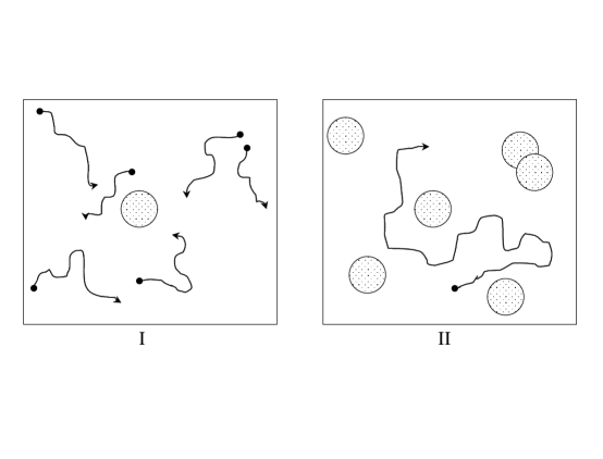
FIG. 1.: Sketch of the reaction $A+B\,\longrightarrow\,B$ between a single $A$ with many $B$’s where the circles show the contact radius for the reaction. In the target problem (panel I) a single $A$ is fixed in space and surrounded by mobile $B$’s while in the trapping problem (panel II) the $B$’s are immobile and the $A$ is mobile. In this latter case the static traps $B$’s are distributed according to the Poisson distribution and overlaps may occur.

FIG. 2.: Reduced effective rate constant, $k/k_{\rm eq}$, as a function of the friction coefficient $\gamma$. The data (closed circles) are obtained from Langevin dynamics simulations, the dot-dashed line corresponds to $k_{\rm high}$ given in Eq.(2.30), the long-dashed line to $k_{\rm low}$ given in Eq.(2.46), the solid and dashed lines through the data represent the VMM interpolation in Eq.(2.47) with $A=1.45$ and $A=6$, respectively. The dotted line is $k_{\rm d}/k_{\rm eq}$, where $k_{\rm d}$, given in Eq.(2.29), represents the purely diffusive part (i.e., $\kappa\rightarrow\infty$) of $k_{\rm high}$.

FIG. 3.: Survival probability $S(t)$ as a function of time for various values of $\gamma$. Solid lines correspond to the Langevin dynamics simulations results. For $\gamma=0$, the solid line represents the exact result in Eq.(2.10) and the dashed line $S_{\rm low}(t)$ given in Eq.(2.36). The dot-dashed line is, ${\rm e}^{-2\kappa\,t}$.

FIG. 4.: Reduced steady-state rate constant, $k_{\rm ss}(\varepsilon)/\kappa$, as a function of the dimensionless friction coefficient $\varepsilon=\gamma/c$. Solid line (Eq.(3.4) with $A=6$) is the essentially exact result while the dashed line (Eq.(3.4) with $A=1.45$) is obtained using the approximate theory.

FIG. 5.: One-dimensional reduced steady-state rate constant, $k_{\rm trap}(\varepsilon)/\kappa$, for the trapping problem as a function of the dimensionless friction coefficient $\varepsilon=\gamma/c$. The solid line represents the exact result (Eq.(3.4) with $A=6$), the dot-dashed line corresponds to $k_{\rm targ}(\varepsilon)/\kappa$ given in Eq.(5.2) for the target problem, the dashed line to $k_{\rm low}(\varepsilon)/\kappa$ given in Eq.(5.4) with $A=1.45$, and the long-dashed line represents the VMM interpolation in Eq.(5.7).

FIG. 6.: Three-dimensional reduced rate constant, $k_{\rm low}(\lambda)/\kappa$, in the low friction regime as a function of the parameter $\lambda=2\pi\varepsilon/3\phi$. The closed circles are obtained from numerical solution of Eq.(5.13) , the solid line corresponds to expression in Eq.(5.17) and the dashed line to the small-$\lambda$ behavior in Eq.(5.16).

   

FIG. 7.: Three-dimensional reduced steady-state rate constant, $k_{\rm trap}(\varepsilon,\phi)/\kappa$, for the trapping problem as a function of the dimensionless friction coefficient $\varepsilon=\gamma R/\sqrt{2\pi}$ for two values of the volume fraction of traps $\phi$. The dot-dashed line corresponds to $k_{\rm targ}(\varepsilon,\phi)/\kappa$ given in Eq.(5.10) for the target problem, the dashed line to $k_{\rm low}$ given in Eq.(5.17), and the solid line represents the VMM interpolation in Eq.(5.18).

REFERENCES

• [1] S. A. Rice, Diffusion-Limited Reactions, (Elsevier, Amsterdam, 1985); E. Kotomin and V. Kuzovkov, Modern Aspects of Diffusion-Controlled Reactions, (Elsevier, Amsterdam, 1996).
• [2] H. A. Kramers, Physica 7, 284 (1940); P. Hänggi, P. Talkner and M. Borkovec, Rev. Mod. Phys. 62, 251 (1990).
• [3] V. I. Mel’nikov and S. V. Meshkov, J. Chem. Phys. 85, 1018 (1986); V. I. Mel’nikov, Phys. Rep. 209, 1 (1991).
• [4] T. W. Marshall and E. J. Watson, J. Pys. A: Math. Gen. 18, 3531 (1985); ibid. 20, 1345 (1987).
• [5] M.S. Wang and G.E. Uhlenbeck, Rev. Mod. Phys. 17, 323 (1945).
• [6] C.R. Doering in Unsolved Problems of Noise, ed. C.R.Doering, L.B. Kiss and M.F. Shlesinger, (World Scientific, Singapore, 1997) p. 11 ; J. Masoliver and J.M. Porrà, Phys. Rev. E 53, 2243 (1996).
• [7] D. J. Bicout, A. M. Berezhkovskii, A. Szabo and G. H. Weiss, Phys. Rev. Lett. 83, 1279 (1999).
• [8] P. B. Visscher, Phys. Rev. B 13, 3272 (1976)
• [9] M. A. Abramowitz and I. A Stegun, Handbook of Mathematical Functions, (Dover Publications Inc., New York, 1972).
• [10] D. J. Bicout and A. Szabo, J. Chem. Phys. 106, 10292 (1997).
• [11] B. Va. Balagurov and V. G. Vaks, Zh. Eksp. Teor. Fiz. 65, 1939 (1973) [Sov. Phys. JETP 38 968 (1974)].
• [12] A. Szabo, J. Phys. Chem. 93, 6929 (1989).
• [13] S. Harris, J. Phys. Chem. 78, 4698 (1983).
Refer to caption