Finite temperature numerical renormalization group
study of the Mott-transition

Abstract

Wilson’s numerical renormalization group (NRG) method for the calculation of dynamic properties of impurity models is generalized to investigate the effective impurity model of the dynamical mean field theory at finite temperatures. We calculate the spectral function and self-energy for the Hubbard model on a Bethe lattice with infinite coordination number directly on the real frequency axis and investigate the phase diagram for the Mott-Hubbard metal-insulator transition. While for $T<T_{\rm c}\approx 0.02W$ ($W$: bandwidth) we find hysteresis with first-order transitions both at $U_{\rm c1}$ (defining the insulator to metal transition) and at $U_{\rm c2}$ (defining the metal to insulator transition), at $T>T_{\rm c}$ there is a smooth crossover from metallic-like to insulating-like solutions.

71.10.Fd, 71.30.+h

I Introduction

During the past decade, the development and application of the dynamical mean field theory (DMFT) has led to a considerable increase in our understanding of strongly correlated electron systems. The DMFT has originally been derived from the limit of infinite spatial dimensionality (or, equivalently, infinite lattice connectivity) of lattice fermion models, such as the Hubbard model [1]. In this limit, the self-energy becomes purely local [2], which is a consequence of the required scaling of the hopping matrix element $t\!=\!t^{\ast}/\sqrt{d}$, with $t^{\ast}$ fixed and $d$ the lattice dimension.

It has been realized in the work of Jarrell [3] and Georges and Kotliar [4] that such a local self-energy can be calculated from a much simpler, but nevertheless highly non-trivial model: the single impurity Anderson model (SIAM) [5]. The self-energy of the SIAM is local because the Coulomb correlation in this model only acts on the impurity site. The difference between the SIAM and the lattice model under consideration is then built in via a self-consistency condition [6]. In this way, the DMFT became a powerful tool for the investigation of various lattice models such as the Hubbard model and the periodic Anderson model (for a review see [6]). The success of this approach, however, depends on the availability of reliable methods for the calculation of the self-energy of an effective SIAM. Perturbative methods, such as the iterated perturbation theory [6] or the non-crossing approximation [7], have been shown to give qualitatively correct results for a variety of physical problems. The numerical implementation of these methods allows one to solve the impurity model with a minimum of computational effort (typically a few seconds on a workstation) so that the relevant parameter space of the model can be scanned very quickly.

However, most of the phenomena of interest in strongly correlated systems are inherently non-perturbative, so that none of the parameters in the Hamiltonian can be regarded as a small perturbation. In general we therefore have to apply non-perturbative methods, even in cases where perturbative approaches such as the iterated perturbation theory or the non-crossing approximation appear to give a complete picture of the solution.

The most widely used non-perturbative method in this context is the quantum Monte-Carlo approach [3, 6]. The advantages of this method are its flexibility (a wide range of physical problems can be studied with only relatively minor changes in the program) and the possibility of obtaining a ‘numerically exact’ solution of $G(\tau)$, the single-particle Green function on the imaginary time axis. The main disadvantage of the quantum Monte-Carlo method is the drastic increase of computation time upon either increasing the Coulomb repulsion $U$ or decreasing the temperature $T$. Furthermore, the analytic continuation of the data on the imaginary time or frequency axis to the real axis represents a difficult and numerically ill-conditioned problem (see [8] for the application of the maximum entropy method to this problem).

Another non-perturbative method applicable here is the exact diagonalization technique (see, e.g., [6, 9, 10]). In this method, the continuous conduction band of the effective SIAM is approximated by a discrete set of states (approximately 8-12 states). The value of $U$ does not impose a problem here as the impurity (together with the conduction electron states) is diagonalized exactly. The main disadvantage of the exact diagonalization technique is its inability to resolve low energy features such as a narrow quasiparticle resonance at the Fermi level.

The above-mentioned restrictions concerning the value of $U$ and $T$, or the low energy resolution, do not apply to the numerical renormalization group method (NRG)[11, 12] which has only recently been used to investigate lattice models within the DMFT [13, 14, 15, 16, 17]. The NRG as well has its drawbacks, which will be discussed in Sec. II of this paper; nevertheless one would expect the NRG to be an ideal tool to calculate the self-energy of the effective Anderson model in the DMFT, simply because it has proven to be very successful in the investigation of the physics of the standard SIAM. For example, the NRG method is able to resolve, both in static and dynamic properties, the exponentially small Kondo scale for large values of $U$ (which can be seen neither in quantum Monte-Carlo nor in exact diagonalization). One can also study in detail the scaling spectrum of the quasiparticle peak [18, 19] and the temperature dependence of transport properties [20, 21] of the SIAM.

Applications of the NRG within the DMFT include the investigation of the Mott-transition [13, 14, 15], the problem of charge ordering in the extended Hubbard model [16], and the formation of the heavy-fermion liquid in the periodic Anderson model [17]. In all these investigations, the temperature was restricted to $T\!=\!0$.

In this paper, we present a study of a strongly correlated lattice model within the DMFT by applying the NRG method at finite temperatures [20, 21]. In particular, we address a problem which has been the topic of an intense debate over the last couple of years: the details of the Mott-transition from a paramagnetic metal to a paramagnetic insulator in the half-filled Hubbard model [6, 15, 22, 23, 24, 25, 26].

The paper is organized as follows: the NRG method is introduced in Sec. II, with particular emphasis on the calculation of finite temperature dynamics. In Sec. III, the previous results for the Mott-transition in the Hubbard model (within DMFT) are discussed. The results from the NRG for the finite temperature Mott-transition are then presented in Sec. IV. The paper is concluded with a summary in Sec. V.

II The Numerical Renormalization Group Method at finite temperatures

A General Concepts

The basic ideas of the NRG method were developed by Wilson for the investigation of the Kondo model [11]. Krishna-murthy, Wilkins, and Wilson [12] later applied the NRG to a related model, the single impurity Anderson model (SIAM) with the Hamiltonian

$$H = \sum_{\sigma}\varepsilon_{\rm f}f^{\dagger}_{\sigma}f_{\sigma}+Uf^{\dagger}_{\uparrow}f_{\uparrow}f^{\dagger}_{\downarrow}f_{\downarrow}$$ (2)

$$+\sum_{k\sigma}\varepsilon_{k}c^{\dagger}_{k\sigma}c_{k\sigma}+\sum_{k\sigma}V\Big{(}f^{\dagger}_{\sigma}c_{k\sigma}+c^{\dagger}_{k\sigma}f_{\sigma}\Big{)}\ .$$

In the model (2), $c_{k\sigma}^{(\dagger)}$ denote annihilation (creation) operators for band states with spin $\sigma$ and energy $\varepsilon_{k}$, $f_{\sigma}^{(\dagger)}$ those for impurity states with spin $\sigma$ and energy $\varepsilon_{\rm f}$. The Coulomb interaction for two electrons at the impurity site is given by $U$ and both subsystems are coupled via a hybridization $V$.

The hybridization function

$$\Delta(\omega)=\sum_{k}\frac{V^{2}}{\omega-\varepsilon_{k}}\ ,$$ (3)

is usually assumed to be constant between the band-edges $-D$ and $D$, but will acquire some frequency dependence in the effective Anderson model within the DMFT (the necessary changes in the NRG-procedure due to the non-constant $\Delta(\omega)$ were discussed in [14, 27]).

The first step to set up the renormalization group transformation is a logarithmic discretization of the conduction band: the continuous conduction band is divided into infinitely many intervals $[\xi_{n+1},\xi_{n}]$ and $[-\xi_{n},-\xi_{n+1}]$ with $\xi_{n}=D\Lambda^{-n}$ and $n=0,1,2,\ldots,\infty$. Here, $\Lambda$ is the NRG discretization parameter (typical values used in the calculations are $\Lambda=1.5,\ldots,2$). The conduction band states in each interval are then replaced by a single state. While this approximation by a discrete set of states involves some coarse graining at higher energies, it captures arbitrarily small energies near the Fermi level.

In a second step, this discrete model is mapped on a semi-infinite chain form via a tridiagonalization procedure (for details, see [11, 12] and section 4.2 in [28]). The Hamiltonian of the semi-infinite chain has the following form:

$$H = \sum_{\sigma}\varepsilon_{\rm f}f^{\dagger}_{\sigma}f_{\sigma}+Uf^{\dagger}_{\uparrow}f_{\uparrow}f^{\dagger}_{\downarrow}f_{\downarrow}+\sum_{\sigma}V\Big{(}f^{\dagger}_{\sigma}c_{0\sigma}+c^{\dagger}_{0\sigma}f_{\sigma}\Big{)}$$ (4)

$$+ \sum_{\sigma,n=0}^{\infty}t_{n}\Big{(}c^{\dagger}_{n\sigma}c_{n+1\sigma}+c^{\dagger}_{n+1\sigma}c_{n\sigma}\Big{)}\ .$$ (5)

This form is valid for a general symmetric conduction band density of states. The impurity now couples only to a single fermionic degree of freedom (the $c^{(\dagger)}_{0\sigma}$), with a hybridization $V$. Due to the logarithmic discretization, the hopping matrix elements decrease as $t_{n}\propto\Lambda^{-n/2}$. This means that, in going along the chain, the parameters in the Hamiltonian evolve from high energies (given by $D$ and $U$) to arbitrarily low energies (given by $D\Lambda^{-n/2}$). The renormalization group transformation is now set up in the following way.

We start with the solution of the isolated impurity, i.e., with the knowledge of all eigenstates, eigenenergies, and matrix elements. The first step of the renormalization group transformation is to add the first conduction electron site, set up the Hamiltonian matrices for the enlarged Hilbert space, and obtain the new eigenstates, eigenenergies, and matrix elements by diagonalizing these matrices. This procedure is then iterated. An obvious problem occurs after only a few steps of the iteration. The Hilbert space grows as $4^{N}$ (with $N$ the size of the cluster), which makes it impossible to keep all the states in the calculation. Wilson therefore devised a very simple truncation procedure in which only those states with the lowest energies (typically a few hundred) are kept. This truncation scheme is very successful but relies on the fact that the hopping matrix elements are falling off exponentially. High-energy states therefore do not change the very low frequency behaviour and can be neglected. This procedure gives for each cluster a set of eigenenergies and matrix elements from which a number of physical properties can be derived.

B Finite Temperature Dynamics

Here we want to discuss in detail the calculation of the finite temperature spectral function

$$A_{\sigma}(\omega)=-\frac{1}{\pi}{\rm Im}\ G_{\sigma}(\omega+i\delta^{+})\ ,$$ (6)

with

$$G_{\sigma}(z)=i\int_{0}^{\infty}{\rm d}t\ e^{izt}\langle[f_{\sigma}(t),f_{\sigma}^{\dagger}]_{+}\rangle\ .$$ (7)

From the iterative diagonalization described above, one can easily calculate the spectral functions for each cluster of size $N$ via[29]

$$A_{\sigma N}(\omega) = \frac{1}{Z_{N}}\sum_{nm}\bigg{|}\phantom{\Big{|}}_{N}\Big{<}n\Big{|}f^{\dagger}_{\sigma}\Big{|}m\Big{>}\!\!\phantom{\Big{|}}_{N}\bigg{|}^{2}\delta\big{(}\omega-(E^{N}_{n}-E^{N}_{m})\big{)}$$ (9)

$$\times\left(e^{-\beta E^{N}_{m}}+e^{-\beta E^{N}_{n}}\right)\ .$$

Here $\big{\{}\big{|}n\big{>}_{N}\big{\}}$ and $\big{\{}\big{|}m\big{>}_{N}\big{\}}$ are sets of eigenstates of the Hamiltonian for the cluster of size $N$, $E^{N}_{n}$ and $E^{N}_{m}$ are the corresponding eigenenergies and $Z_{N}$ the grand canonical partition function (the spin index $\sigma$ will be dropped in the following). As the length of the cluster is successively increased, and the $A_{\sigma N}(\omega)$ calculated in each step, Eq. (9) defines a whole set of spectral functions. These data are combined to give spectral functions as shown, e.g., in Fig. 3 in the following way.

Let us first describe the procedure for calculating the $T=0$ spectral function [20, 30]. The diagonalization of the clusters $N=0,1,2,\dots$ yields the excitation spectrum $\omega_{nm}=E_{n}^{N}-E_{m}^{N}$ on a set of decreasing energy scales $\omega_{0}>\omega_{1}>\omega_{2}>\dots$ ($\omega_{N}$ is the smallest scale in the truncated Hamiltonian $H_{N}$, i.e., $\omega_{N}=t_{N}$ and for a flat band one has $\omega_{N}\sim D\Lambda^{-(N-1)/2}$). Excitations $\omega\ll\omega_{N}$ are not described within cluster $N$. They are obtained accurately in subsequent iterations from larger clusters. Similarly, excitations $\omega\gg\omega_{N}$ are outside the energy window for cluster $N$ (whose width is limited on the high energy side by the truncation of the spectrum). Information on these excitations is contained in previous iterations for some smaller cluster $N^{\prime}<N$. It is therefore possible to use Eq. (9) for each $N=0,1,\dots$ to calculate the $T=0$ spectral density at an appropriate set of decreasing frequencies for each cluster. These frequencies are chosen to be $\omega\approx 2\omega_{N}$ within the energy window of the cluster under consideration (whose width, in units of $\omega_{N}$, typically lies in the range 6-10 for $\Lambda=1.5-2.0$).

At finite temperature, the above procedure is modified as follows. For a given temperature $T$, which we identify with $T_{M}\approx\omega_{M}$ for some $M$, one evaluates the spectral density in Eq. (9) at the same characteristic frequencies $\omega=2\omega_{N}$ as those used for the $T=0$ calculation, down to a minimum frequency corresponding to $\omega\approx T=T_{M}$. Compared to the $T=0$ calculation, many more excitations will contribute at finite $T$, as shown in Fig. 1. When $\omega=2\omega_{N}$ becomes comparable to or smaller than the temperature of interest, $T=T_{M}$, it is clear that excitations will start to contribute to the spectral density at frequency $\omega$ which are not contained in cluster $N$. It is still possible to calculate the spectral density at frequencies $\omega=2\omega_{N}$ such that $-T_{M}\leq\omega\leq+T_{M}$ by using the cluster of size $M$ corresponding to the temperature. This is achieved by broadening the $\delta$-functions in the spectrum of cluster $M$ with broadening functions of width $T$ (see below). This gives a very good estimate of the leading contribution to the spectral density for all frequencies $|\omega|\leq T$. It recovers, for example, the known Fermi liquid relations for transport quantities of the Anderson model [20, 21]. Due to the limited resolution, proportional to $T_{M}$, the above scheme will, however, tend to broaden the spectral densities too much at higher temperatures.

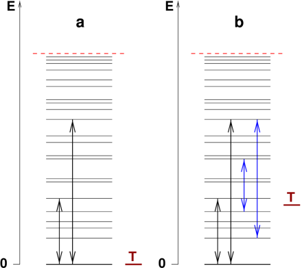
FIG. 1.: The spectrum of many-body excitations measured with respect to the ground-state energy $E_{\rm g}\!=\!0$, and the possible transitions contributing to the single-particle spectral function. a) For $T\!=\!0$, only transitions between the ground-state and excited states are possible; b) for $T\!>\!0$, transitions between excited states are possible as well. The dotted line indicates the cut-off in the spectrum due to the truncation of states.

This is not a problem for the finite temperature spectral densities presented in this paper. The reason, as we shall see below, is that the width of the Kondo resonance in the effective impurity model is always very much larger than the temperatures of interest (typically by a factor of 10 larger).

The above scheme becomes increasingly accurate as the temperature is lowered, eventually connecting continuously the finite and zero temperature spectral densities as $T\rightarrow 0$.

There are several ways to put together the discrete information from the clusters in order to arrive at continuous curves for spectral densities. One approach [20, 21] replaces the delta functions in Eq. (9) by appropriate broadening functions (see Eq. (10–11)) and evaluates the spectral densities at the characteristic frequencies defined above. It is also possible to first combine information on the discrete spectra from successive clusters ($N$ and $N+2$, to avoid even/odd effects) and then broaden the spectra [14]. Below, we describe this latter approach, which we used to obtain most results in this paper. A comparison between the two approaches gave only minor differences in the results for the spectral function.

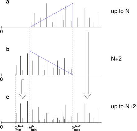
FIG. 2.: Superposition of the $\delta$-peaks in the spectral density of all clusters up to length $N$ [see (a)] with the $\delta$-peaks of the cluster of length $N+2$ [see (b)]. This procedure gives the spectral information contained in all clusters up to length $N+2$ [see (c)]. The spikes indicate the weight of the $\delta$-functions in the spectral density, and the lines in (a) and (b) correspond to the weighting function as described in the text. The $\delta$-peaks in the interval $[\omega_{\rm min}^{N+2},\omega_{\rm min}^{N}]$ and for $\omega>\omega_{\rm max}^{N+2}$ appearing in (c) are identical to those appearing in (a) and (b), repectively, as indicated by the arrows.

The starting point is the set of $\delta$-peaks obtained for a small cluster of size $N$ where the truncation is not yet effective (see Fig. 2a). The spectral distribution for the cluster of length $(N+2)$ is shown in Fig. 2b. The minimal frequency appearing in the spectrum for the cluster of length $(N+2)$, $\omega_{\rm min}^{N+2}$, is reduced approximately by a factor of $\Lambda$ compared to the frequency $\omega_{\rm min}^{N}$, while the maximal frequency $\omega_{\rm max}^{N+2}$ is now determined by the number of states retained after truncation. From the two sets of $\delta$-peaks we keep those peaks which are in the interval $[\omega_{\rm min}^{N+2},\omega_{\rm min}^{N}]$ and above $\omega_{\rm max}^{N+2}$. The peaks in the overlapping region $[\omega_{\rm min}^{N},\omega_{\rm max}^{N+2}]$ are taken from both the previous clusters and the one of length $N+2$, and are added with a weighting function which is, for simplicity, just a linear function with values from 0 to 1 for arguments between $\omega_{\rm min}^{N}$ and $\omega_{\rm max}^{N+2}$ (for the previous clusters) and with values from 1 to 0 (for the cluster of length $N+2$) [31]. The resulting set of $\delta$-peaks is shown in Fig. 2c and can then be used to further iterate this procedure (with the cluster of length $N+4$, and so on), up to the cluster of length $M$ defined by $T=T_{M}$.

The resulting spectrum is still discrete. To visualize the distribution of spectral weight it is convenient to broaden the $\delta$-peaks using appropriate broadening functions. For the results shown in this paper we used a Lorentzian

$$\delta(\omega-\omega_{n})\rightarrow\frac{1}{2\pi}\frac{b}{(\omega-\omega_{n})^{2}+b^{2}}\ ,$$ (10)

with width $b=0.6T$ for $\omega_{n}<4T$ and a Gaussian on a logarithmic scale

$$\delta(\omega-\omega_{n})\rightarrow\frac{e^{-b^{2}/4}}{b\,\omega_{n}\sqrt{\pi}}\exp\left[-\frac{(\ln\omega-\ln\omega_{n})^{2}}{b^{2}}\right]\ ,$$ (11)

with width $b=0.3$ for $\omega_{n}>4T$.

So far, we have not made any reference to the application of the NRG to the effective Anderson model in the DMFT. The necessary steps are described in [14] for the case of $T\!=\!0$ and can be used for finite temperatures equally well. In particular, the expression of the self-energy via

$$\Sigma_{\sigma}(\omega)=U\frac{F_{\sigma}(\omega)}{G_{\sigma}(\omega)},$$ (12)

with the correlation function $F_{\sigma}(\omega)=\langle\!\langle f_{\sigma}f^{\dagger}_{\bar{\sigma}}f_{\bar{\sigma}},f^{\dagger}_{\sigma}\rangle\!\rangle_{\omega}$ holds for both $T\!=\!0$ and $T\!>\!0$ (for a discussion of the advantage of using Eq. (12) for the calculation of $\Sigma(\omega)$, see [14]).

Let us now comment on the choice of temperatures used in the calculations reported in this paper. It is clear from the above discussion that the temperatures are chosen to lie within the excitation spectrum of the cluster $M$ for which the NRG iteration is terminated. Keeping the position of $T_{M}$ within the excitation spectrum constant, one has to reduce $T_{M}$ by a factor $\Lambda$ when the largest cluster is of length $M+2$. This defines a discrete set of temperatures $T_{N}=T_{M}\Lambda^{(N-M)/2}$ for which we perform the NRG calculations.

For a variety of applications within the DMFT one would certainly prefer to vary the temperature continuously (to find, e.g., the critical temperatures for a phase transition). Such a continuous variation is difficult within NRG. It is certainly possible to achieve a large variation in temperature by a modest variation in $\Lambda$ and using a fixed length of the cluster (due to the exponential dependence of $T_{M}$ on $\Lambda$). The results obtained in this way would, however, contain different systematic errors, as the accuracy of the NRG is enhanced upon reducing $\Lambda$. One should therefore try to correct this $\Lambda$-dependence, e.g., by extrapolating the results to $\Lambda=1$. We have not attempted to correct for the $\Lambda$-dependence and instead worked with a fixed $\Lambda=1.64$ and different cluster sizes (the number of states retained after truncation is 600, not counting degeneracies).

III The Mott-Hubbard Metal-Insulator Transition

Let us now turn to the Mott metal-insulator transition [22, 32] from a paramagnetic metal to a paramagnetic insulator. This transition is found in various transition metal oxides, such as $\rm V_{2}O_{3}$ doped with Cr [33]. The mechanism driving the Mott-transition is believed to be the local Coulomb repulsion $U$ between electrons on the same lattice site, although the details of the transition should also be influenced by lattice degrees of freedom. The simplest model to investigate the correlation driven metal-insulator transition is the one-band Hubbard model [34, 35, 36]

$$H=-\sum_{ij\sigma}t_{ij}(c^{\dagger}_{i\sigma}c_{j\sigma}+c^{\dagger}_{j\sigma}c_{i\sigma})+U\sum_{i}c^{\dagger}_{i\uparrow}c_{i\uparrow}c^{\dagger}_{i\downarrow}c_{i\downarrow}\ ,$$ (13)

where $c^{\dagger}_{i\sigma}$ ($c_{i\sigma}$) denote creation (annihilation) operators for a fermion on site $i$ and the $t_{ij}$ are the hopping matrix elements between site $i$ and $j$ [37]. Despite its simple structure, the solution of this model turns out to be an extremely difficult many-body problem. The situation is particularly complicated near the metal-insulator transition where $U$ and the bandwidth are roughly of the same order such that perturbative schemes (in $U$ or $t$) are not applicable.

The existence of a metal-insulator transition in the paramagnetic phase [38] of the half-filled Hubbard model has been known since the early work of Hubbard [34]. The details of the transition, however, remained unclear, except in the particular case of dimension $d=1$, where the transition occurs at $U=0^{+}$ [22, 39]. Even in the opposite limit of infinite dimensions, where a numerically exact solution of the Hubbard model is in principle possible, a general consensus concerning the details of the transition scenario has not been reached so far.

Neglecting the transition to an antiferromagnetic phase or suppressing it by frustration [6], two coexisting solutions are found in DMFT at very low temperatures, one insulating and one metallic [40]. The transition is then of first order, even in the absence of a coupling to lattice degrees of freedom. The scenario of a first-order transition was first proposed in Refs. [41, 42], within calculations based on the iterated perturbation theory and exact diagonalization. It was later confirmed by the NRG for $T=0$ [15] and quantum Monte-Carlo calculations for $T>0$ [24, 43]. Criticism of this scenario can be found in Refs. [25, 44, 45, 46].

The results from the NRG for the $T\!=\!0$ metal-insulator transition can be summarized as follows (for details see [15]). On approaching the transition from the metallic side, a typical three-peak structure appears in the spectral function, with upper and lower Hubbard bands at $\omega\approx\pm U/2$ and a quasiparticle peak at $\omega=0$. The width of the quasiparticle peak vanishes for $U\to U_{\rm c2}$, leaving behind two well-separated Hubbard peaks (see Fig. 2 in [15]). Although the NRG is not able to resolve a small spectral weight between the Hubbard peaks, the results indicate that the gap opens discontinuously (see also [6]). On decreasing $U$, the transition from the insulator to the metal occurs at a lower critical value $U_{\rm c1}$, where the gap vanishes. Concerning the numerical value of $U_{\rm c2}\approx 1.47W$ ($W$: bandwidth) excellent agreement with the result from the projective self-consistent method [47, 6] is found.

The extension of the NRG to $T>0$ will now be used to determine the full shape of the hysteresis region non-perturbatively.

IV Results

A Spectral function for $T>T_{\rm c}$

Figure 3 shows the spectral function $A(\omega)$ for various values of $U$ at $T=0.0276W$. This is above the temperature of the critical point (which we estimate as $T_{\rm c}\approx 0.02W$), so that there is no real transition but a crossover from a metallic-like to an insulating-like solution. As already found in Refs.[6, 23], the crossover region is nevertheless very narrow, with a very rapid suppression of the quasiparticle peak. This is seen also in the NRG results (Fig. 3) when $U$ is increased from $U=1.05W$ to $U=1.20W$. The spectral weight of the quasiparticle peak is gradually redistributed and shifted to the upper (lower) edge of the lower (upper) Hubbard band. An additional structure within the Hubbard bands, as reported in [6, 23], is not found and would be very difficult to see due to the limited resolution of the NRG at higher frequencies.

The inset of Fig. 3 shows the $U$-dependence of the value of the spectral function at zero frequency $A(\omega\!=\!0)$. For higher values of $U$, the spectral density at the Fermi level is still finite and vanishes only in the limit $U\to\infty$ (or for $T\to 0$, provided that $U>U_{\rm c2}(T=0)$).

The $U$-dependence of $A(\omega\!=\!0)$ is shown in Fig. 4a for different temperatures. As discussed in Sec. II, the temperatures are chosen as $T_{m}=T_{1}\cdot\Lambda^{m}$, with $T_{1}=0.0168W$ and $m=0,1,2,3$, ($\Lambda=1.64$ is used for all results shown in this paper; the number of states retained after truncation is 600, not counting degeneracies). The derivative of $A(\omega\!=\!0)$ with respect to $U$,

$$A^{\prime}(\omega\!=\!0)\equiv\frac{\partial A(\omega=0,U)}{\partial U}\ ,$$ (14)

is plotted in Fig. 4b. The $U$-value where $|A^{\prime}(\omega\!=\!0)|$ reaches its maximum defines a characteristic interaction strength $U^{\ast}$ for the crossover from metallic-like to insulating-like behavior in the region $T\!>\!T_{\rm c}$; for the definition of $U_{c1,2}$ for $T\!<\!T_{\rm c}$, see below. Furthermore, the width $\Delta U$ of the crossover region can be defined as the width at half-height of the peak in $A^{\prime}(\omega\!=\!0)$.

FIG. 3.: Spectral function for the half-filled Hubbard model for various values of $U$ at $T=0.0276W>T_{c}$ (in the crossover region). The crossover from the metal to the insulator occurs via a gradual suppression of the quasiparticle peak at $\omega\!=\!0$. The inset shows the $U$-dependence of $A(\omega\!=\!0)$, in particular the rapid decrease for $U\approx 1.1W$.

FIG. 4.: (a): The $U$-dependence of $A(\omega\!=\!0)$ for different temperatures; the data for $T\!=\!0.0168W<T_{\rm c}$ show a very small hysteresis, not visible on this scale. The other three sets of data are for $T>T_{\rm c}$. (b): The derivative of $A(\omega\!=\!0,U)$ with respect to $U$ for the same temperatures as in (a).

Upon lowering the temperature, the width $\Delta U$ rapidly decreases and vanishes at the critical temperature $T_{\rm c}$, since $A^{\prime}(\omega\!=\!0)$ diverges at $T_{\rm c}$ (this feature has already been discussed in [48]). A precise value for $T_{\rm c}$ cannot be given as we are presently not able to vary the temperature within NRG continuously. The critical temperature is estimated as $T_{\rm c}\approx 0.02W$, as a very small hysteresis is still present for $T=0.0168W$ (on the scale of Fig. 4, $U_{\rm c1}$ and $U_{\rm c2}$ cannot be distinguished).

The $U^{\ast}$ as defined above slowly decreases upon increasing the temperature. This is not at variance with the opposite trend observed in Refs. [6, 7, 23] (in Ref. [23], the slope of $U^{\ast}$ changes sign at $T\approx 0.25W$) and depends on the definition of $U^{\ast}$. Taking $U^{\ast}$ as, e.g., the value of $U$ where $A(\omega\!=\!0)$ has dropped to 1% of its value at $U\!=\!0$ would result in an increase of $U^{\ast}$ upon increasing the temperature.

B Breakdown of Fermi Liquid versus Metal-Insulator Transition

We now discuss the question of how to define a useful criterion for the metal-insulator transition at finite temperatures. At zero temperature a suitable criterion is the vanishing, with increasing $U$, of the quasiparticle weight

$$Z=\frac{1}{1-\left.\frac{\partial{\rm Re}\Sigma(\omega)}{\partial\omega}\right|_{\omega=0}}\ .$$ (15)

The physical meaning of $Z$ is clear for the paramagnetic state at $T=0$, where the system is either a Fermi liquid (for $U<U_{\rm c}$) or an insulator (for $U>U_{\rm c}$). The vanishing of $Z$ therefore marks the metal-insulator transition at $T=0$, as discussed, e.g, in [6, 15]. This criterion, however, cannot be taken over straightforwardly to finite temperatures, since for $T>0$ the breakdown of the Fermi liquid state and the appearence of the insulating state do not coincide. Although this point has been noted before in the literature (see, e.g., [49, 23]), the vanishing of $Z$ has been used as (one) criterion for the occurence of the metal-insulator transition in [23]. It should be noted that the definition of $Z$ used in the finite temperature quantum Monte-Carlo calculations of Ref. [23] is different from Eq. (15) since $\left.\partial{\rm Re}\Sigma(\omega)/\partial\omega\right|_{\omega=0}$ was approximated by ${\rm Im}\Sigma(i\omega_{0})/\omega_{0}$, with $\omega_{0}$ the first Matsubara frequency.

To elucidate this point, it is instructive to discuss the behavior of the self-energy in the crossover region from the metallic-like to the insulating-like solution. The real and imaginary part of $\Sigma(\omega)$ are shown in Fig. 5, for the same temperature and $U$ values as in Fig. 3. For $U=1.05W$ and $U=1.10W$ the imaginary part shows the characteristic structure of the self-energy for a Fermi liquid (with the $\omega^{2}$ dependence for small frequencies and the falling off at higher frequencies which leads to a two-peak structure), but with a rapidly increasing scattering rate at $\omega\!=\!0$ for increasing $U$. The two-peak structure gradually evolves into a structure with a well-pronounced peak at $\omega\!=\!0$ characteristic for an insulating solution (a vanishing $A(\omega\!=\!0)$ would correspond to a $\delta$-function in ${\rm Im}\Sigma(\omega)$). Note that for $U\geq 1.15W$ the value of ${\rm Im}\Sigma(\omega=0)$ is much larger than the $T^{2}$-term observed for $T\to 0$. Hence, the mechanism for the strong scattering at $\omega\!=\!0$ is not the quasiparticle-interaction but is caused by the bare local Coulomb repulsion, which destroys the Fermi liquid behavior for $U\geq 1.15W$. For $U=1.15W$ there is still a narrow dip in ${\rm Im}\Sigma(\omega)$ at $\omega\!=\!0$ corresponding to the remnant of the quasiparticle peak seen in Fig. 3.

FIG. 5.: Imaginary part (a) and real part (b) of the self-energy for the same temperature ($T=0.0276W$) and $U$-values as in Fig. 3. The slope of ${\rm Re}\Sigma(\omega)$ changes sign at the same $U$-value for which the peak at $\omega\!=\!0$ appears in Im$\Sigma(\omega)$.

For $U=1.05W$ and $U=1.10W$, the corresponding real part of $\Sigma(\omega)$ shows the typical Fermi liquid behavior with a negative slope at $\omega\!=\!0$. Upon further increasing the $U$, however, the slope of ${\rm Re}\Sigma(\omega)$ changes sign right at the $U$-value where the peak at $\omega\!=\!0$ appears in Im$\Sigma(\omega)$; this is obvious from the Kramers-Kronig transformation which connects real and imaginary part. Note that the $1/\omega$-behavior in ${\rm Re}\Sigma(\omega)$ for larger frequencies is not visible on this scale.

From the full frequency dependence of $\Sigma(\omega)$ on the real axis one can easily perform the analytic continuation to $\Sigma(z)$ for any value of $z$ in the upper complex plane:

$$\Sigma(z)=-\frac{1}{\pi}\int{\rm d}\omega^{\prime}\frac{{\rm Im}\Sigma(\omega^{\prime})}{z-\omega^{\prime}}\ .$$ (16)

In particular for $z=i\omega$ and $\omega$ real, Eq. (16) gives the real and imaginary parts of the self-energy on the imaginary frequency axis (the analytic continuation from the imaginary to the real frequency axis, however, is much more delicate, see, e.g., [8]). The result for Im$\Sigma(i\omega)$ is shown in Fig. 6, for the same parameters as in Figs. 3 and 5. The circles indicate the value of Im$\Sigma(i\omega_{n})$ for the Matsubara frequencies

$$\omega_{n}=\frac{\pi}{\beta}(2n+1),\ \ \ \ n=0,1,2,\ldots\ .$$ (17)

As the self-energy $\Sigma(z)$ is defined on the whole imaginary frequency axis, not only for the Matsubara frequencies, one can, for instance, check the trivial condition ${\rm Im}\Sigma(i\omega)={\rm Im}\Sigma(\omega)$ for $\omega\to 0$.

FIG. 6.: Imaginary part of the self-energy, Im$\Sigma$, on the imaginary frequency axis for the same parameters as in Figs. 3 and 5. The values of Im$\Sigma$ for the Matsubara frequencies are indicated by the circles. The inset focuses on the change of sign of the slope in Im$\Sigma(i\omega)$ for values of $U=1.1W$ up to $U=1.17W$ (from top to bottom).

Furthermore, the slope of ${\rm Im}\Sigma(i\omega)$ for $\omega\to 0$ is identical to the slope of the real part of $\Sigma(\omega)$. As a consequence, the same change in the slope of the self-energy is visible in both Figs. 5b and 6. The inset of Fig. 6 illustrates this for a smaller frequency range and a narrow mesh of $U$-values from $U=1.1W$ up to $U=1.17W$ (from top to bottom).

This behavior of the self-energy has drastic consequences for the notion of a quasiparticle weight $Z$ in the crossover regime. We see that the application of Eq. (15) to the self-energies as obtained in Figs. 5 and 6 leads to unphysical results for $U\geq 1.15W$. Due to the change of sign in $\left.\frac{\partial{\rm Re}\Sigma(\omega)}{\partial\omega}\right|_{\omega=0}$ upon increasing $U$, the $Z$ from Eq. (15) starts increasing again and even diverges at a particular value of $U$ for which the derivative of the self-energy is equal to one. For larger values of $U$, $Z$ becomes negative and approaches zero from below for $U\to\infty$. Apparently, the use of Eq. (15) does not make sense for $U\geq 1.15W$ [50] which is due to the fact the the concept of quasiparticles itself breaks down in the crossover regime. The quasiparticle weight is therefore not an appropriate measure for the metal-insulator transition in the whole parameter space. Note also that in the crossover region, the weight of the remnant of the quasiparticle peak is not associated to $Z$.

Whereas there is no unique criterion for a characteristic value $U^{\ast}$ for $T>T_{\rm c}$, critical values for $U$ can nevertheless be defined for $T<T_{\rm c}$ via the value of $U$ at which $A(\omega=0)$ changes discontinuously.

C Spectral function for $T<T_{\rm c}$

Figure 7 shows the spectral function $A(\omega)$ in the hysteresis region for $T\!=\!0.0103W$, both for increasing $U$ (Fig. 7a) and decreasing $U$ (Fig. 7b). The results are shown for a very fine mesh of $U$-values close to $U_{\rm c2}\approx 1.21W$ and $U_{\rm c1}\approx 1.14W$.

FIG. 7.: Spectral function for $T\!=\!0.0103W$; (a): increasing $U$ (b): decreasing $U$; the transitions at $U_{\rm c2}\approx 1.21W$ and $U_{\rm c1}\approx 1.14W$ are characterized by a significant redistribution of spectral weight and a jump in $A(\omega\!=\!0)$ (see also Fig. 8) .

In both cases, the transition is of first order, i.e., associated with a discontinuous redistribution of spectral weight. The hysteresis effect is further illustrated in the $U$-dependence of $A(\omega\!=\!0)$ for $T\!=\!0.0103W<T_{c}$ (Fig. 8).

Whereas the critical values $U_{\rm c1}$ and $U_{\rm c2}$ can be easily defined by the jump in $A(\omega\!=\!0)$, the calculation of the actual thermodynamic transition requires the knowledge of the free energy $F$ of both metallic and insulating solutions. The determination of $F$ goes beyond the scope of this paper. There is no way of directly calculating $F$ within the NRG approach, so one has to determine the free energy via integrating over a path from a particular point in the $(U,T)$-plane for which the free energy is known, up to the actual values of $U$ and $T$. However, the knowledge of the $U_{\rm c}(T)$ for the actual thermodynamic transition will not alter the fact that the transition is of first order.

FIG. 8.: $U$-dependence of $A(\omega\!=\!0)$ for $T\!=\!0.0103W$; solid line: increasing $U$, dashed line: decreasing $U$.

D Phase diagram

Let us finally discuss the phase diagram for the Mott metal-insulator transition in the very low temperature region.

In Fig. 9, the dashed lines for $T>T_{\rm c}$ indicate the position and width of the crossover region as calculated from the NRG data of Fig. 4. The open circles and squares are the NRG-results for $U_{\rm c1}(T)$ and $U_{\rm c2}(T)$, respectively. As the NRG calculations cannot, so far, be performed for arbitrary values of $T$, we cannot give a precise value for the critical point. The $U_{\rm c2}(T)$ nicely extrapolates to the previously obtained value for $T\!=\!0$ [15]; the same is true for $U_{\rm c1}(T)$. Note that the value for $U_{\rm c1}(T\!=\!0)=1.195W$ plotted here is slighly reduced as compared to the originally published value $U_{\rm c1}(T\!=\!0)=1.25W$ [15]. This is due to the different value for $\Lambda$, the number of states and the broadening used here.

Figure 9 also contains recent quantum Monte-Carlo results of Joo and Oudovenko [26] (filled symbols), as well as the result from the iterated perturbation theory [6] which tends to overestimate both $U_{\rm c1}(T)$ and $U_{\rm c2}(T)$. The phase boundaries obtained from the NRG are below the values obtained from the quantum Monte-Carlo results. Concerning the NRG values, it is well-known that due to the logarithmic discretization the NRG tends to underestimate the effective hybridization [51] (hence underestimating the value of $U$ necessary to overcome the kinetic energy). This effect has, e.g., been studied in the context of the quantum phase-transition from the local moment to the strong coupling phase in the soft-gap Anderson model [19]. For the transition in this model, the value of $U_{\rm c}$ for $\Lambda\!=\!2.0$ is about 5% below the extrapolated value for $\Lambda\to 1$; more importantly, the $U_{\rm c}(\Lambda)$ is a perfectly straight line from $\Lambda\!=\!1.4$ to $\Lambda\!=\!3.0$.

FIG. 9.: Results for the phase diagram of the Mott transition obtained from different methods: NRG (open symbols), quantum Monte-Carlo (QMC, filled symbols) and iterated perturbation theory (IPT, solid lines). The dashed lines for $T>T_{\rm c}$ indicate the position and width of the crossover region as calculated from the data of Fig. 4.

A similar $\Lambda\to 1$ extrapolation is difficult to perform for the metal-insulator transition studied here, since already a very large number of DMFT iterations is necessary to determine a single value of $U_{\rm c}(\Lambda)$. Calculations of $U_{\rm c1}$ and $U_{\rm c2}$ for one value of $T$ with $\Lambda\!=\!1.64$ and $\Lambda\!=\!2.0$ at least show the expected trend, i.e., a slight increase of the $U_{\rm c}$’s with decreasing $\Lambda$.

Taking into account the unavoidable numerical errors in both procedures, the agreement between NRG and quantum Monte-Carlo results for the phase-boundary is seen to be very good; the agreement can even be further improved [43].

V Summary

In this paper we presented results from the numerical renormalization group method (NRG) for the finite temperature Mott transition in the Hubbard model on a Bethe lattice within dynamical mean field theory. For the crossover region $T>T_{\rm c}$, the quasiparticle peak in the spectral function gradually vanishes upon increasing $U$ and the imaginary part of the self-energy develops a sharp peak at $\omega=0$. Associated with this is a change of sign of Re$\Sigma(\omega)$ at $\omega=0$. As a consequence, the behaviour of the quasiparticle weight can no longer be used as a criterion for the transition at finite temperature.

For $T<T_{\rm c}\approx 0.02W$, we find two coexisting solutions in the range $U_{\rm c1}(T)<U<U_{\rm c2}(T)$. The values for the critical $U$ can be determined for arbitrarily small temperatures, in contrast to the quantum Monte-Carlo method which is so far restricted to $T>W/150$. The critical $U_{\rm c1}(T)$ and $U_{\rm c2}(T)$ are characterized by a redistribution of finite spectral weight in the spectral function.

We therefore obtain a consistent picture for the Mott metal-insulator transition from a paramagnetic metal to a paramagnetic insulator in the whole parameter regime. The results are in very good agreement with those from other non-perturbative methods (the quantum Monte-Carlo method and the projective self-consistent method) in their respective ranges of applicability.

There are still several questions left for further investigations. A continuous variation of the temperature within the NRG requires a better understanding of the $\Lambda$-dependence of the results. The NRG also allows the calculation of a variety of dynamic and transport properties in the whole parameter regime, such as dynamic susceptibility and optical conductivity. A generalization of the NRG method to antiferromagnetic phases and the Hubbard model away from half-filling is in progress.

Acknowledgements: It is a pleasure to acknowledge fruitful discussions with N. Blümer, W. Hofstetter, A.P. Kampf, and Th. Pruschke. Two of us (RB and TAC) would like to thank the Isaac Newton Institute for Mathematical Sciences for hospitality where part of this work was done. We also acknowledge the support of the Deutsche Forschungsgemeinschaft through the Sonderforschungsbereich 484.

REFERENCES

- [1] W. Metzner and D. Vollhardt, Phys. Rev. Lett. 62, 324 (1989).
- [2] E. Müller-Hartmann, Z. Phys. B 74, 507 (1989).
- [3] M. Jarrell, Phys. Rev. Lett. 69, 168 (1992).
- [4] A. Georges and G. Kotliar, Phys. Rev. B 45, 6479 (1992).
- [5] P.W. Anderson, Phys. Rev. 124, 41 (1961).
- [6] A. Georges, G. Kotliar, W. Krauth, and M.J. Rozenberg, Rev. Mod. Phys. 68, 13 (1996).
- [7] Th. Pruschke, D.L. Cox, and M. Jarrell, Phys. Rev. B 47, 3553 (1993).
- [8] M. Jarrell and J.E. Gubernatis, Physics Reports 269, 133 (1996).
- [9] M. Caffarel and W. Krauth, Phys. Rev. Lett. 72, 1545 (1994).
- [10] W. Krauth, Phys. Rev. B 62, 6860 (2000).
- [11] K.G. Wilson, Rev. Mod. Phys. 47, 773 (1975).
- [12] H.R. Krishna-murthy, J.W. Wilkins, and K.G. Wilson, Phys. Rev. B 21, 1003 (1980); ibid. 21, 1044 (1980).
- [13] O. Sakai and Y. Kuramoto, Solid State Commun. 89, 307 (1994).
- [14] R. Bulla, A.C. Hewson, and Th. Pruschke, J. Phys.: Condens. Matter 10, 8365 (1998).
- [15] R. Bulla, Phys. Rev. Lett. 83, 136 (1999).
- [16] R. Pietig, R. Bulla, and S. Blawid, Phys. Rev. Lett. 82, 4046 (1999).
- [17] Th. Pruschke, R. Bulla, and M. Jarrell, Phys. Rev. B 61, 12799 (2000).
- [18] H.O. Frota and L.N. Oliveira, Phys. Rev. B 33, 7871 (1986).
- [19] R. Bulla, M.T. Glossop, D.E. Logan, and Th. Pruschke, J. Phys.: Condens. Matter 12, 4899 (2000).
- [20] T.A. Costi and A.C. Hewson, Philos. Mag. B 65, 1165 (1992).
- [21] T.A. Costi, A.C. Hewson, and V. Zlatić, J. Phys.: Condens. Matter 6, 2519 (1994).
- [22] F. Gebhard, The Mott Metal-Insulator Transition, Springer Tracts in Modern Physics Vol. 137 (Springer, Berlin 1997).
- [23] J. Schlipf, M. Jarrell, P.G.J. van Dongen, S. Kehrein, N. Blümer, Th. Pruschke, and D. Vollhardt, Phys. Rev. Lett. 82, 4890 (1999).
- [24] M.J. Rozenberg, R. Chitra, and G. Kotliar, Phys. Rev. Lett. 83, 3498 (1999).
- [25] R. Noack and F. Gebhard, Phys. Rev. Lett. 82, 1915 (1999).
- [26] J. Joo and V. Oudovenko, preprint cond-mat/0009367.
- [27] R. Bulla, Th. Pruschke, and A.C. Hewson, J. Phys.: Condens. Matter 9, 10463 (1997).
- [28] A.C. Hewson, The Kondo Problem to Heavy Fermions (Cambridge Univ. Press, Cambridge 1993).
- [29] In the presence of a magnetic field, a different choice of spectral representation, based on using the reduced density matrices of clusters , is required, see W. Hofstetter, Phys. Rev. Lett. 85, 1508 (2000).
- [30] O. Sakai, Y. Shimizu, and T. Kasuya, J. Phys. Soc. Jpn. 58, 3666 (1989).
- [31] The precise form of the weighting function turns out to be unimportant for the final result, e.g., the form of the spectral function; the idea is here to reduce the weight of those -peaks which are at the edges of the spectrum of each cluster.
- [32] N.F. Mott, Proc. Phys. Soc. London A 62, 416 (1949); Metal-Insulator Transitions, 2nd ed. (Taylor and Francis, London 1990).
- [33] D.B. McWhan and J.P. Remeika, Phys. Rev. B 2, 3734 (1970); D.B. McWhan, A. Menth, J.P. Remeika, Q.F. Brinkman, and T.M. Rice, Phys. Rev. B 7, 1920 (1973).
- [34] J. Hubbard, Proc. R. Soc. London A 276, 238 (1963).
- [35] M.C. Gutzwiller, Phys. Rev. Lett. 10, 59 (1963).
- [36] J. Kanamori, Prog. Theor. Phys. 30, 275 (1963).
- [37] For a discussion of the validity of this simplest possible model, see: S.Y. Ezhov, V.I. Anisimov, D.I. Khomskii, and G.A. Sawatzky, Phys. Rev. Lett. 83, 4136 (1999); F. Mila, R. Shiina, F.-C. Zhang, A. Joshi, M. Ma, V. Anisimov, and T.M. Rice, Phys. Rev. Lett. 85, 1714 (2000); K. Held, G. Keller, V. Eyert, D. Vollhardt, and V.I. Anisimov, preprint cond-mat/0011518.
- [38] The hopping matrix elements in Eq. (13) are assumed to be chosen in such a way that antiferromagnetic long-range order is suppressed completely [6].
- [39] E.H. Lieb and F.Y. Wu, Phys. Rev. Lett. 20, 1445 (1968).
- [40] Although the term insulator is only strictly defined for , we denote a solution as insulating if it shows well separated upper and lower Hubbard peaks with a only a small spectral weight at the Fermi level.
- [41] A. Georges and W. Krauth, Phys. Rev. B 48, 7167 (1993).
- [42] M.J. Rozenberg, G. Kotliar, and X.Y. Zhang, Phys. Rev. B 49, 10181 (1994).
- [43] N. Blümer, P.G.J. van Dongen, and D. Vollhardt, in preparation.
- [44] S. Kehrein, Phys. Rev. Lett. 81, 3912 (1998).
- [45] D. E. Logan and P. Nozières, Phil. Trans. R. Soc. London A 356, 249 (1998).
- [46] P. Nozières, Eur. Phys. J. B 6, 447 (1998).
- [47] G. Moeller, Q. Si, G. Kotliar, M. Rozenberg, and D. S. Fisher, Phys. Rev. Lett. 74, 2082 (1995).
- [48] G. Kotliar, E. Lange, and M.J. Rozenberg, Phys. Rev. Lett. 84, 5180 (2000).
- [49] M.J. Rozenberg, G. Kotliar, H. Kajueter, G.A. Thomas, D.H. Rapkine, J.M. Honig, and P. Metcalf, Phys. Rev. Lett. 75, 105 (1995).
- [50] This value of , valid for , depends on temperature.
- [51] C. Gonzalez-Buxton and K. Ingersent, Phys. Rev. B 54, 15614 (1996).