Correlation effects in a simple model of small-world network

Abstract

We analyze the effect of correlations in a simple model of small world network by obtaining exact analytical expressions for the distribution of shortest paths in the network. We enter correlations into a simple model with a distinguished site, by taking the random connections to this site from an Ising distribution. Our method shows how the transfer matrix technique can be used in the new context of small world networks.

I Introduction

Real networks, like social networks, neural networks, power-grids, and documents in World Wide Web (WWW)mil ; fhcs ; n ; ajb , can be modeled neither by totally random networks nor by regular ones (see n ; w ; ab and references therein for review). While locally they are clustered as in regular networks, remote sites have often the chance of being connected via shortcuts, as in random graphs, hence reducing the average distance between sites in the network.
In a regular networks with $N$ vertices, the average shortest path between two vertices $<l>$ and the clustering coefficient $C$ scale respectively as $<l>\sim N$ , and $C\sim 1$. The clustering coefficient $C$ is defined as the average ratio of the number of existing connections between neighbors of a vertex to the total possible connections among them. In random networks, however we have $<l>\sim\log N$ and $C\sim 1/N$ er ; bol .
The properties of many real networks, are a hybrid of these two extremes, that is in these networks one has $<l>\sim logN$, and $C\sim 1$. These two effects called collectively small world effect, are attributed respectively to the presence of shortcuts and the many inter-connections that usually exist between the neighboring nodes of such networks k1 ; mg ; lm .
In 1998, Watts and Strogatz ws introduced a simple model of network showing the small world behavior, which since then has been investigated as a model of interconnections in many different contexts, ranging from epidemiology ak ; z ; mdl , to polymer physics sc ; sab ; jb , and evolution and navigation bb1 ; k2 ; plh , The original model of Watts and Strogatz contained a free parameter $p$, by varying which one could interpolate between random and irregular networks. Their model, called hereafter the WS model, consists of a ring of $N$ sites in which each site is connected to its $2k$ nearest neighbors, hence making a regular network. After this stage, each bond is re-wired with probability $p$ to another randomly chosen site. The value of $p$ tunes the amount of randomness introduced into the network. Since there is a finite probability of disconnecting the whole network in this way, Newman and Watts nw modified the model by replacing the re-wiring stage by just addition of shortcuts between randomly chosen sites on the ring. Since then many more variants and generalizations of small world networks and their different characteristics ( e.g. their topology, the properties of random walks on them, etc.) have been studied. Of particular interest are three classes of studies. The first class , in which the static properties of small world networks have been investigated bw ; mn ; kas ; ka ,the second class ,where dynamical aspects have been studied m ; jsb and the third class,in which evolving networks are considered deb ; ke in order to generate small world networks with various connectivity distributions ,including scale free distributions.
In this letter we want to consider another variant of the small world network, one in which correlation of neighboring nodes in making connections to remote sites is taken into account(ie;the presence of a shortcut between two sites affects other shortcuts in the neighborhood) . For example a node need not make a short-cut to a remote site if there is such a connection in its neighborhood. In such networks then, correlations play an important role. However to perform such a study by exact non-mean field methods requires a simplification in the original model. We assume all shortcuts are made via a distinguished site at the center of the ring. More than being a simplification, this type of network has practical relevance in many situations where a central distinguished site governs all the remote interconnections. We note in passing that such central sites ,accommodating a large number of connections, may exist either in the architecture of the original networks or else may appear dynamically in evolving networks bb2 . In this way we assume that contrary to the original model,dm , the two configurations in fig.1 , both with 5 shortcuts are not equiprobable.

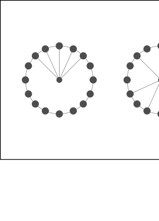
Figure 1: Two configurations which have different weights in our calculations but equal weights in dm .

II The model and Small world quantities

We consider a circular network of $N$ vertices with a distinguished central site 2. The links on the ring have unit length. Each shortcut connecting any two sites on the ring is also of unit length. We assign a random variable $s_{i}\in\{0,1\}$ to each site $i$ of the ring. This random variable is $1$ or $0$ according to whether the site is connected to the center or not,fig.2. Any configuration of these spin variables corresponds to one and only one configuration of connections to the center. For example in fig.1 if each bond is independently connected to the center with probability $p$, then the probabilities of both configurations are equal and proportional to $p^{5}(1-p)^{11}$. In general and in the absence of correlations we will have:

$$P=\frac{1}{Z}(\frac{p}{1-p})^{s_{1}+s_{2}+\cdots s_{N}},$$ (1)

where Z is a normalization constant. To consider correlations we generalize the above distribution to an Ising type distribution, namely to:

$$P\{s_{i}\}=\frac{1}{Z}\biggl{(}{\prod_{i=1}^{N}r^{s_{i}}\zeta^{s_{i}s_{i+1}}}\biggr{)}.$$ (2)

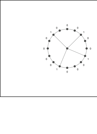
Figure 2: A simple model of small world networks.

For $\zeta=1$ and $r=\frac{p}{1-p}$ we obtain the original model of dm . The value of $\zeta$ controls the correlations.
First let us consider the directed model, i.e; the links on the circle are directed, say clockwise. Looking at fig.3, we consider a typical configuration like the one shown in this figure ,in which the nearest shortcuts to sites $1$ and $j$ are connected at sites $i$ and $k$. This configuration reduces the distance between sites $1$ and $j$ by an amount $k-i-1$. Not that the sites between $i$ and $k$ may or may not be connected to the center. In any such configuration the quantity $X_{i,k}(1,j)$ defined as:

$$(1-s_{1})\cdots(1-s_{i-1})s_{i}s_{k}(1-s_{k+1})\cdots(1-s_{j}),$$ (3)

takes the value $1$.The average of this quantity gives the probability of such a configuration.In order to find the probability of the shortest path between sites $1$ and $j$ to be equal to $l$, we have to sum over all those configurations which give such a shortest path . For $l\neq j-1$ the above probability is given by:

$$p(1,j;l)=\sum_{i=1}^{l}<X_{i,j+i-l-1}(1,j)>,$$ (4)

where we have used $<..>$ for averaging over configurations .

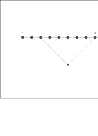
Figure 3: A typical configuration which decreases $l_{1j}$.

Normalization determines $P(1,j;j-1)$ via:

$$p(1,j;j-1)=1-\sum_{l=1}^{j-2}p(1,j;l).$$ (5)

The probability that the shortest path between two arbitrary vertices be of length $l$, is obtained from:

$$p(l)=1/N\sum_{j=l+1}^{N}p(1,j;l).$$ (6)

Now the average shortest path between two randomly chosen sites is:

$$<l>=\sum_{l=1}^{N-1}lp(l).$$ (7)

All the above quantities can be calculated by the transfer matrix method,in which we write the unnormalized distribution 2 as product of matrix elements of a matrix $T$ :

$$T=\left(\begin{array}[]{cc}1&\sqrt{r}\\ \sqrt{r}&r\zeta\end{array}\right)$$ (8)

with eigenvalues:

$$\lambda_{\pm}=\frac{1}{2}[1+r\zeta\pm\sqrt{(1-r\zeta)^{2}+4r}].$$ (9)

The partition function is $Z=\lambda_{+}^{N}+\lambda_{-}^{N}$ and the number of connections per site is given by:

$$p:=\frac{r}{N}\frac{\partial}{\partial r}\ln Z.$$ (10)

We now consider the continuum limit of the lattice, where the number of vertices goes to infinity and the lattice constant goes to zero as $\frac{1}{N}$ so that the periphery of the lattice is kept constant at $1$ . We then set: $j/N\longrightarrow x,k/N\longrightarrow s,i/N\longrightarrow t$ $l/N\longrightarrow z$ and $NX_{i,k}(1,j)\longrightarrow X(t,s)(x)$ where the explicit form of the function $X(t,s)(x)$ will be determined later. We will then have $0\leq x,t,s,z\leq 1$. Here $x$ is the distance along the ring.
Furthermore we take $Np(1,j,l)\rightarrow{\cal Q}(x,z)$ ,therefore :

$${\cal Q}(x,z) = \int_{0}^{z}{X(t,x+t-z)(x)}\rm{d}t,$$ (11)

$${\cal Q}(z) = \int_{z}^{1}{{\cal Q}(x;z)}\rm{d}x,$$ (12)

where ${\cal Q}(x,z)dz$ is the probability that two points whose distance along the ring is $x$ have a shortest distance between $z$ and $z+dz$. Then ${\cal Q}(z)dz$ is the probability that the shortest path between any two points be between $z$ and $z+dz$ . So $\int_{0}^{1}dzQ(z)=1$ and finally :

$$<z> = \int_{0}^{1}{z{\cal Q}(z)}dz.$$ (13)

II.1 The scaling limit

Intuitively we expect that in the scaling limit, when $N\longrightarrow\infty,{\rm and}\ \ r=\frac{r_{0}}{N}$, if we keep $\zeta$ finite, then the number of connections to the center remains finite and in an infinite lattice the configurations of these connections become quite sparse and hence correlations can not play a role, at least to leading order. Exact calculation also verifies this expectation. Here we will consider a different scaling limit where $N\longrightarrow\infty,{\rm and}\ \ r=\frac{r_{0}}{N}$ while $\zeta=\zeta_{0}N$. This means that the tendency of an individual one of whose neighbors has been connected to the center, depends also on the total population. This assumption is not far from reality, specially in cases where the center approves a limited amount of connections and the applicants ,competing for connections, are aware of this restriction. It turns out that the model shows three distinct behavior according to the value of the parameter $r_{0}\zeta_{0}$.
For $r_{0}\zeta_{0}>1$ we will have:

$$\lambda_{+} = r_{0}\zeta_{0}+\frac{r_{0}}{N(r_{0}\zeta_{0}-1)},$$ (14)

$$\lambda_{-} = 1-\frac{r_{0}}{N(r_{0}\zeta_{0}-1)},$$ (15)

and from (10) we find:

$$p=1+O(\frac{1}{N}),$$ (16)

which means that the whole lattice is filled with connections. Also for $r_{0}\zeta_{0}=1$ we obtain $p=\frac{1}{2}$,which is also far from small world regime. To be in the small world regime, we should keep $r_{0}\zeta_{0}<1$ , which is the case that we will study in detail.
In this case we have:

$$\lambda_{+} = 1+\frac{r_{0}}{N(1-r_{0}\zeta_{0})},$$ (17)

$$\lambda_{-} = r_{0}\zeta_{0}-\frac{r_{0}}{N(1-r_{0}\zeta_{0})}.$$ (18)

Also from (10) we find the total number of connections to be the finite value:

$$M_{0}:=Np=\frac{r_{0}}{(1-r_{0}\zeta_{0})^{2}}.$$ (19)

To calculate $X_{i,k}(1,j)$ we note that since $p\rightarrow 0$ as $\frac{1}{N}$ , the value of these quantities where either or both of $i$ and $k$ take the extreme values $1$ or $j$ are suppressed. Using the transfer matrix technique, we obtain from (2 , 3) that for $1<i<k<j$,

$$<X_{i,k}(1,j)>=T_{00}^{i-2}T_{01}(T^{k-i})_{11}T_{10}T_{00}^{j-k-1}(T^{N-j+1})_{00}=r(T^{k-i})_{11}(T^{N-j+1})_{00},$$ (20)

where $T_{ij}^{m}=<i|T|j>^{m}$ and $(T^{m})_{ij}=<i|T^{m}|j>$. Diagonalizing $T$, using (8 , 9), and taking the continuum limit, we find after some algebra:

$$X(s-t)(x)=M^{2}e^{-Mx}e^{M(s-t)},$$ (21)

where $M:=\frac{r_{0}}{1-r_{0}\zeta_{0}}$. Inserting this value in (11) and integrating we find:

$${\cal Q}(x;z)=zM^{2}e^{-Mz},$$ (22)

$${\cal Q}(z)=z(1-z)M^{2}e^{-Mz}+(1+zM)e^{-Mz},$$ (23)

Turning to (13) it is obtained :

$$<z>=\frac{1}{M}\big{(}2+e^{-M}\big{)}-\frac{3}{M^{2}}\big{(}1-e^{-M}\big{)}.$$ (24)

As expressed in dm , these relations already hint at the emergence of a type of small world behaviour, i.e: with connecting only 10 sites the average shortest path is reduced from $\frac{1}{2}$ to 0.17, connecting an extra 10 sites reduces this value to 0.09.
We see that as far as $\zeta_{0}<\frac{1}{r_{0}}$, the effect of correlations is only to modify the relations of dm by replacing $M_{0}$, the actual number of connections , with an effective one $M$. Expressing $M$ in terms of $M_{0}$ and $\zeta_{0}$ alone, we find: $M_{0}=M(1+M\zeta_{0})$, which means that for low values of $\zeta_{0}$, $M\sim M_{0}$ while for large values of $\zeta_{0}$ the effective number of connections scales as the square root of the actual number of shortcuts, $M\sim\sqrt{\frac{M_{0}}{\zeta_{0}}}$. This effect reflects the tendency of the shortcuts to get clustered under the influence of correlations. Hence correlations tend to decrease the small world effect, since the connections tend to bunch into clusters.

III Undirected and clustered networks

As far as we have $N\rightarrow\infty$ and $M_{0}=$finite, we can generalize our results to the cases where

a)-the network has no preferred direction

and

b)- each site of the ring is connected to $2k$ of its neighbors.

In this limit, in going from one site of the ring to another one, one travels mostly along the ring. Thus denoting the average shortest paths for the above cases respectively by $\ll z\gg_{a}$ and $\ll z\gg_{b}$ we have

$${\ll z\gg}_{a}=\frac{1}{2}\ll z\gg\hskip 14.22636pt,\hskip 14.22636pt{\ll z\gg}_{b}=\frac{1}{k}\ll z\gg,$$ (25)

from which we obtain

$${\cal Q}_{a}(z)=2{\cal Q}(2z)\hskip 28.45274pt0\leq z\leq\frac{1}{2}$$ (26)

and

$${\cal Q}_{b}(z)=k{\cal Q}(kz)\hskip 28.45274pt0\leq z\leq\frac{1}{k}.$$ (27)

And finally ,for the clustered undirected model one will have

$${\cal Q}_{ab}(z)=2k{\cal Q}(2kz)\hskip 28.45274pt0\leq z\leq\frac{1}{2k}.$$ (28)

IV Conclusion

We have considered the effect of correlations in a simple model of small world network, and shown that they generally decrease the small world effect, since under this condition the connections tend to bunch into clusters. More concretely in our simple model the effect of correlations which are controlled by a parameter $\zeta_{0}$, is to reduce (for large $zeta_{0}$) the actual number of shortcuts $M_{0}$ to an effective one $M\sim\sqrt{\frac{M_{0}}{\zeta_{0}}}$, indicating a clustering of connections to bunches in the lattice.
Therefore it seems that the optimal way of designing a small world network would be with equidistant long-range connections and in order to see the small world effect and lower the average shortest path, one is better to use algorithms which anticorrelate the connections.
We have derived our results by exact analytical methods, and have shown how the transfer matrix technique can be used for obtaining such properties as average shortest path, or the distribution of shortest paths in a model of small world network. For all this we have been forced to study a restricted class of models. No doubt by doing computer simulations one can study these effects in a much broader class of models.

References

- (1) S.N.Dorogovtsev and J.F.F.Mendes, Europhys. Lett. 50,1 (2000).
- (2) S. Milgram, Psychology Today 2: 60-67 (1967).
- (3) L.F.L-Fernandez,R.Huerta,F.Corbacho and J.A.Siguenza,Phys. Rev. lett. 84(12):2758-2761 Mar 2000.
- (4) M. E. J. Newman, Small Worlds,J. Stat. Phys. 101(3-4):819-841 Nov 2000.
- (5) R. Albert, H. Jeong, and A. L. Barabasi, Nature, 401 :130-131 (1999).
- (6) D. J. Watts, Small Worlds, Princeton University Press (Princeton)(1999).
- (7) R.Albert and A.L.Barabasi,cond-mat/0106096.
- (8) P. Erdös and A. Renyi, Pulicationes Mathematicae, 6: 290-297 (1959).
- (9) B. Bollaoas, Random Graphs Academic Press (New York)(1985).
- (10) R.Kasturirangan,cond-mat/9904055 .
- (11) N.Mathias and V.Gopal,Art.no.021117 Phys. Rev. E 6302(2):1117-+ Part 1 ,Feb 2001.
- (12) V.Latora and M.Marchiori,To appear in Phys. Rev. Lett.
- (13) D.J.Watts and S.H.Strogatz , Nature 393,440(1998).
- (14) M.Kuperman and G.Abramson,Phys. Rev. Lett. vol. 86 :2909-2912 (2001).
- (15) D.H.Zanette, cond-mat/0105596.
- (16) S. C. Manrubia, Jordi Delgado and Bartolo Luque, Europhys. Lett. 53(5):693-699 ,Mar 2001.
- (17) P.Sen and B.K.Chakrabarti, cond-mat/0105346.
- (18) A.Scala,L.A.N.Amaral and M.Barthelemy,Europhys. Lett. 55(4):594-600 ,Aug 2001.
- (19) S.Jespersen and A.Blumen, Phys. Rev. E 62(5):6270-6274 Part A ,Nov 2000.
- (20) F.Bagnoli and M.Bezzi,art.no.021914 Phys. Rev. E 6402(2):1914-+ Part 1 ,Aug 2001.
- (21) J.M.Kleinberg,Nature ,vol 406,845(2000).
- (22) A.R.Puniyani,R.M.Lukose and B.A. Huberman,cond-mat/0107212.
- (23) M.E.J.Newman and D.J.Watts, Phys. Rev. E 60: 7332-7342 (1999).
- (24) A.Barrat and M.Weigt.2000, Europ. Phys. J. B 13, 547 (2000).
- (25) C.Moore and M.E.J.Newman, Phys. Rev. E 62: 7059-7064 (2000).
- (26) R.V.Kulkarni,E.Almaas and D.Stroud,Phys. Rev. E 61, 4268 (2000).
- (27) M. Kuperman and G.Abramson, Phys. Rev. E 6404(4), art.no.047103:7103-+ Part 2,Oct 2001.
- (28) R.Monasson,Europ. Phys. J. B 12(4):525-567,Dec 1999.
- (29) S.Jespersen,I.M.Sokolov and A.Blumen,Phys. Rev. E 62(3):4405-4408 Part B,Sep 2000.
- (30) J. Davidsen,H. Ebel and S. Bornholdt,cond-mat/0108302.
- (31) K. Klemm and V. M. Eguiluz,cond-mat/0107607.
- (32) G. Bianconi and A. L. Barabasi,Phys. Rev. Lett. 86(24):5632-5635 ,Jun 2001.